completion based on topological gradient and
fast marching algorithms - Application to
inpainting and segmentation
Y. Ahipo1, D. Auroux2, L. D. Cohen3, and M. Masmoudi4
1
Spring Technologies, Toulouse, France
2
Laboratoire J. A. Dieudonn´e, Universit´e de Nice Sophia Antipolis, France
3
CEREMADE, UMR CNRS 7534, Universit´e Paris Dauphine, France
4
Institut de Math´ematiques de Toulouse, France cohen@ceremade.dauphine.fr
Abstract. We combine in this paper the topological gradient, which is a powerful method for edge detection in image processing, and a variant of the minimal path method in order to find connected contours. The topological gradient provides a more global analysis of the image than the standard gradient, and identifies the main edges of an image. Several image processing problems (e.g. inpainting and segmentation) require continuous contours. For this purpose, we consider the fast marching algorithm, in order to find minimal paths in the topological gradient image. This coupled algorithm quickly provides accurate and connected contours. We present then two numerical applications, to image inpaint-ing and segmentation, of this hybrid algorithm.
Keywords: topological gradient, fast marching, contour completion
1
Introduction
Contour detection is a major issue in image processing. For instance, in classifi-cation and segmentation, the goal is to split the image into several parts. This problem is strongly related to the detection of the connected contours separating these parts. It is quite easy to detect edges using local image analysis techniques, but the detection of continuous contours is more complicated and needs a global analysis of the image.
Several image processing problems like image inpainting and denoising (or enhancement) are classically solved without detecting edges and contours. The goal of image enhancement is to denoise the image without blurring it. A clas-sical idea is to identify the edges in order to preserve them, and to smooth the image outside them. In this particular case, contour completion is not prereq-uisite, as the quality of the result is not much related to the completeness of
the identified edges. But for most of the other image processing problems (seg-mentation, inpainting, classification), the detection of connected contours can drastically simplify the resolution and improve the quality of the results. For instance, the image segmentation problem is a very good example, as the goal is to split the image into its characteristic parts. In other words, one has to find connected contours, which define different subsets of the image.
For solving all these problems, various approaches have been considered in the literature. By lack of space, we will only give a general quote on the most commonly used models: the structural approach by region growing, the stochastic approaches and the variational approaches, which are based on various strategies like level set formulations, the Mumford-Shah functional, active contours and geodesic active contours methods or wavelet transforms.
Another approach to define edges as cracks, is based on the topological asymptotic analysis [8, 2]. The goal of topological optimization is to look for an optimal design (i.e. a subset) and its complementary. Finding the optimal sub-domain is equivalent to identifying its characteristic function. At first sight, this problem is not differentiable. But the topological asymptotic expansion gives the variation of a cost function j(Ω) when we switch the characteristic function from one to zero in a small region [9]. More precisely, we consider the perturbation of the main domain Ω by the insertion of a small crack (or hole) σρ: Ωρ= Ω\σρ, ρ
being the size of the crack. The topological sensitivity theory provides then an asymptotic expansion of the considered cost function when the size of the crack tends to zero. It takes the general form: j(Ωρ) − j(Ω) = f (ρ)g(x) + o(f (ρ)),
where f (ρ) is an explicit positive function going to zero with ρ, and g(x) is the topological gradient at point x. Then, in order to minimize the criterion (or at least its first order expansion), one has to insert small cracks at points where the topological gradient is the most negative. An efficient edge detection technique, based on the topological gradient, was introduced in [8]. But the identified edges are usually not connected, and the results can be degraded. This is beyond the scope of this paper to give a more detailed description, which can be found in [8, 2].
In the inpainting problem, we assume that there is a hidden part of the image, and our goal is to recover this part from the known part of the image. Here the interior of the missing part is not empty, it is neither a random set nor a narrow line, we assume that it is a quite large part of the image. This problem has been widely studied and some of the most common approaches are: learning approches (neural networks, radial basis functions, . . . ) [13, 14], minimization of an energy cost function based on a total variation norm [3], morphological component analysis methods separating texture and cartoon [7].
We now consider the crack detection technique, within the framework of the identification of the image edges, either in the hidden part of the image for the inpainting application, or in the whole image for the segmentation application [2]. The topological asymptotic analysis provides very quickly the location of the edges, as they are precisely defined as the most negative points of the topological gradient. The main issue of such a technique is the need for connected contours.
This can easily be understood as the hidden part of the image is filled using the Laplace operator in each subdomain of the missing zone, and a discontinu-ous contour would lead to some blurred reconstruction. Up to now, one had to threshold the topological gradient with a not too small value, in order to identify connected contours, but this leads to thick identified edges, and also to consider more noisy points as potential edges. In order to overcome this limitation, we consider a minimal path technique for connecting the edges.
Minimal paths have been first introduced for finding the global minimum of active contour models, using the fast marching technique [4]. They have then been used to find contours or tubular structures and also for perceptual grouping using a path or a set of paths minimizing a functional [5, 15, 6, 12, 10]. In our case, the energy to be minimized will be proportional to the topological gradient. As the topological gradient takes its minimal values on the edges of the image, the idea is indeed to find contours for contour completion from the various minima and small values of the topological gradient.
For perceptual grouping, a set of keypoints is considered as starting points and a set of minimal paths connecting some pairs of these keypoints is considered as a contour completion. This approach is extremely satisfactory in 2D problems, with quite few key points. It is also extremely fast. In 3D images, minimal paths find tubular structures, but in order to identify minimal surfaces, this approach is much more difficult to consider. It was dealt in the case of a surface connecting two curves in [1]. We only consider here the 2D case.
The application of the minimal path technique to the topological gradient al-lows us to obtain an automatic identification of the main (missing or not) edges of the image. These edges will be continuous, by construction, and will allow us to simply apply the Laplace operator to fill the image for inpainting appli-cations, or will directly provide the segmented image, with very good results. Another advantage of this technique is to be very fast, as it does not degrade the O(n. log(n)) complexity of the topological gradient based algorithm intro-duced in [2]. We also refer to these citations for the inpainting and segmentation algorithms by topological asymptotic expansion, and for a detailed presenta-tion of the topological gradient. We assume here that the topological gradient is available.
In section 2, we propose an algorithm based on the minimal path and fast marching techniques in order to identify the valley lines of the topological gra-dient, which correspond to the main edges of the image. Then, we report the results of several numerical experiments in section 3. We also compare this hy-brid scheme with the fast marching algorithm applied to the standard gradient. Two particular image processing problems are considered: segmentation and in-painting. Finally, some conclusions are given in section 4.
2
A 2D algorithm based on the minimal paths and fast
marching methods
2.1 Minimal paths
In this section, we describe the standard minimal path technique, adapted to our needs. We refer to [4] for more details about the minimal paths method.
In the following, let Ω be the considered image domain. We assume that Ω is a regular subset of R2. In order to compute some minimal paths, we need to
define a potential function, measuring in some sense for any point of Ω the cost for a path to contain this point. As we want to identify paths in the topological gradient image, and considering that this potential function must be positive, we will define a potential function as follows:
P(x) = g(x) − min
y∈Ω{g(y)}, ∀x ∈ Ω, (1)
where g is the topological gradient, defined in all the domain Ω. We can see that the points where the topological gradient g reaches its minimal values are quite costless. We denote by C(s) a path, or curve, in the image, where s represents the arclength. We now define a functional, measuring the cost of such a path:
J(C) = Z
C
(P (C(s)) + α) ds, (2)
where α is a positive real coefficient that represents regularization. In our ap-plications, α is usually very small, as the goal is to connect the most negative parts of the topological gradient, whatever the Euclidean distance is.
We now consider a key point x0∈ Ω of the image, and x will represent any
point of the image. The energy J(C) of a given path C can be seen as a distance between the two endings of C, weighted by the potential function. The goal is to find the minimal energy integrated along the path C. We can now define the weighted distance between key point x0 and point x by
D(x; x0) = inf C∈A(x,x0) J(C) = inf C∈A(x,x0) Z C (P (C(s)) + α) ds, (3) where A(x, x0) is the set of all paths going from point x0to point x in the image.
The distance D(x; x0) introduced in equation (3) is then simply the instant t
at which the front, initialized at key point x0, reaches point x. An efficient way
to compute this distance function is the fast marching algorithm, and is justified by the fact that the distance satisfies the following Eikonal equation
k∇xD(x; x0)k = P (x) + α, (4)
with the initialization D(x0; x0) = 0. We refer to [4, 11, 1, 15, 10, 12] for more
details about the fast marching technique and the justification of equation (4). If n is the size of the image, the complexity of this fast marching method is bounded by O(n. log(n)), which is also the complexity of the topological gradient algorithm.
2.2 Multiple minimal paths
The main issue is now to extend this minimal path technique to more than one keypoint, in order to connect several points. This is exactly what we need, in order to connect the identified edges by the topological gradient, as we have many identified keypoints (for example all negative local minima of the topological gradient) that we want to connect. As explained in [5], the first step of a multiple minimal path algorithm is to reduce the set of keypoints, for computational reasons. Moreover, the selected keypoints should not be too close one to each other. One usually chooses a total number N of keypoints, and the first one. Then the N − 1 other keypoints can be chosen for instance as described in [5].
The next step consists of connecting these N points. One has to compute the distance function from each of these key points, and the common minimal paths algorithms provide then the Vorono¨ı diagram of the distance and the corresponding saddle points (minimal distance along the edges of the diagram, maximal distance from the keypoints). The Vorono¨ı diagram defines a partition of the image in as many subsets as the number of keypoints. Each subset is defined by the set of points that are closer to the corresponding keypoint than to all others. The saddle points minimize the distance function on the edges of the diagram: minimal distance on the edge, maximal distance to the keypoints. It is useful to compute these saddle points to save computation time since it reduces the domain of the image where the fast marching computes or updates the weighted distance map..
Finally, the idea is to consider the saddle-points as initial conditions for minimizing the distance function. For each saddle-point as an initial point, a minimization is performed towards each of the two corresponding keypoints (re-call that the saddle-points are located at the interface between two subsets of the Vorono¨ı diagram). Each minimization produces a path between the saddle-point (initial condition) and a keypoint (local minimum of the distance function). This step is usually called back-propagation, as it consists of a gradient descent from the saddle-point, back to the linked keypoints. The back-propagation step is straightforward as there is no local minimum of the distance function, except the keypoints. The union of all these paths gives a continuous path, connecting the keypoints together.
The interesting part of the approach introduced in [5] is that each keypoint should not be connected to all the others, but only to at most two others, as we are looking for a set of closed connected path. Thus, the keypoints have to be ordered automatically in a way such that they are only connected to the other keypoints that are closest to them in the energy sense [5]. For this reason, we sort all the saddle-points from smaller to larger distance, and we first try to connect the pairs of keypoints corresponding to the saddle-points of smallest distance. These keypoints are indeed more likely to be connected than distant keypoints, corresponding to saddle-points of large potential. Once the close keypoints are connected, we repeat the process with the new closest pairs of keypoints, provided each point remains connected to at most two other ones. At the end of the process, all the keypoints are connected to at most two other
keypoints, and the union of all minimal paths between the keypoints represents one (or several) continuous contour of the image. An interesting feature of this method is that the key points are by construction widely distributed around.
If all the selected keypoints are on the same contour of the image, we are almost sure that at the end, they will all be connected together and we will retrieve the corresponding contour, as the potential function (related to the topological gradient) is very low on this contour. If, on the contrary, one keypoint is not part of the contour, the large values of the topological gradient, and hence of the potential function, will isolate this keypoint from the other ones, and it will not disturb the contour completion process.
2.3 Main Algorithm
The hybrid algorithm we propose is then the following:
Fast marching algorithm applied to the topological gradient: • Compute the topological gradient of the image.
• Set N the number of keypoints and choose the N keypoints: the main one will be for example the global minimum of the topological gradient, the other ones being the most negative local minima of the topological gradient. • Compute the distance function (3) with all these keypoints, and the
corre-sponding Vorono¨ı diagram.
• Compute the set of saddle-points: on each edge of the Vorono¨ı diagram, determine the point of minimal distance.
• Sort all these points of minimal distance, from smaller to larger distance. • For each of these saddle-points, from smaller to larger distance, check if it
will not be used to connect two keypoints, one of which is already connected to two other keypoints.
• If this is not the case, perform the back-propagation from this point: use this saddle-point as an initialization for a descent type algorithm in order to connect the two corresponding keypoints.
It is straightforward to see that this algorithm converges, and that at con-vergence, all the keypoints are connected to at most two other keypoints. This provides one or several continuous contours, containing the keypoints. As the first keypoint is usually the global minimum of the topological gradient, it is on one of the main edges of the image. Consequently, using this algorithm, we can identify this edge. Then, it is possible to restart the algorithm, using other keypoints that are not on this identified edge, by initializing for instance the first keypoint as the minimum of the topological gradient outside the neighborhood of this edge.
3
Numerical experiments
3.1 Numerical results for 2D segmentation
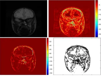
We first consider a two dimensional grey level image, represented in figure 1 on the left. The opposite of the Euclidian norm of its standard gradient is
repre-Fig. 1.Top: Original image (left); L2
norm of its (standard) gradient (right). Bottom: Topological gradient (left); edges by thresholding the topological gradient (right)
sented on the right. Note that we represent its opposite in order to have com-parable images with the topological gradient, which has negative values (see below).
The topological gradient is represented on the bottom part of figure 1. As it quantifies in a global way whether a pixel is part of an edge or not, it is much less sensitive to noise and small variations of the image than the standard gradient. For instance, the topological gradient takes much larger absolute values on the edges than outside, contrary to the standard gradient. In the segmentation algorithm presented in [2], the idea until now was to threshold the topological gradient in order to define the edge set. Such a threshold is represented in figure 1 on the right side. One can see that, in order to obtain at least the main connected edge, the threshold coefficient has been set to a low value, leading to add many unwanted points to the edge set, but also to thick edges. And even in this case, the main contour is not totally continuous. Then, the idea is to apply the variant of the fast marching algorithm we proposed in section 2.3.
Using an automatic thresholding for identifying the most negative values of the topological gradient, figure 2 shows on the left the set of points (or admissible keypoints, in blue), in which we will choose the keypoints for the minimal path algorithm. The first keypoint is set to the minimum of the topological gradient. Then, we have set the number of keypoints to N = 3. From the first keypoint, we start the minimal path algorithm, and we choose the second keypoint as being the point (in the admissible set) maximizing the weighted distance to the first keypoint. Then, we start again the minimal path algorithm from these two points, and we set the third keypoint in a similar way. These three keypoints are represented by black points in the left side of figure 2. Note that the keypoints can
Fig. 2. Admissible set of points in blue, and 3 keypoints automatically selected in black (left); distance function (middle) computed from these 3 keypoints with the fast marching algorithm and identified minimal paths between the keypoints. Correspond-ing Vorono¨ı diagram, with the 3 keypoints and saddle points ; (right).
also be (manually) provided by the user, for instance with the aim of identifying a specific edge of the image.
From these keypoints, we run the minimal path algorithm, in order to com-pute the distance map. Figure 2 shows on the middle this distance function. One can clearly see that the distance does not correspond to the Euclidean metric in the plane, as the distance remains very small on the common edge of the 3 key-points, whereas it takes much larger values outside. The corresponding Vorono¨ı diagram is represented in figure 2 on the right. The three keypoints are still rep-resented by black points. Each color represents the subset Ωi of points that are
closer to keypoint i than to the others. For any i 6= j, we consider the interface Γij = Ωi∩ Ωj between two subsets of the Vorono¨ı diagram. Γij represents then
the set of points equidistant from keypoints i and j. We now minimize the dis-tance function on Γij in order to find a saddle-point: same distance to keypoints
i and j, minimal distance on Γij. These saddle points are represented by blue
points on the right side of figure 2.
From these saddle points, the idea is finally to perform a descent-type algo-rithm in order to minimize the distance function from the saddle points to the keypoints. We consider a saddle-point on an edge Γij as an initial condition for
two minimizations of the distance function, one towards each of the correspond-ing keypoints (i and j). Each of these two minimizations provides a continuous path from the saddle-point to one of the two keypoints. The union of these two paths connects the two keypoints. This process is done for all pairs of consecutive keypoints.
The final set of paths is represented in green on the distance function in figure 2 (middle). The three keypoints are also represented (in white). These paths correspond to the contour of the original image that contains the 3 keypoints. By applying again this algorithm, with other keypoints (selected outside the first identified contours), it is possible to detect other contours of the image.
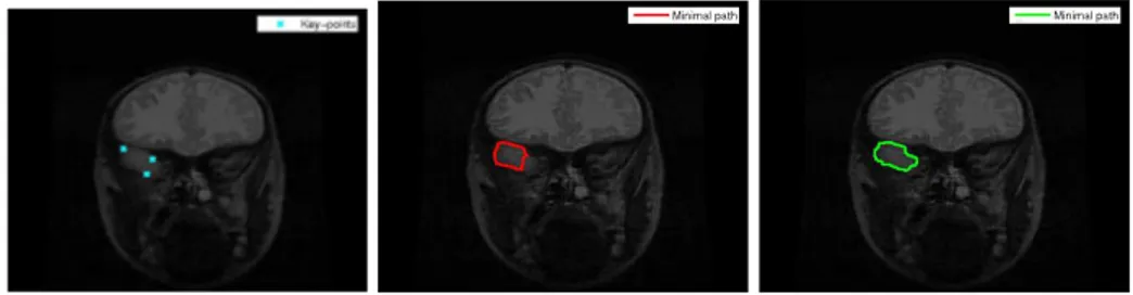
Finally, we illustrate the fact that the topological gradient provides better information about the edges of the image than the standard gradient, as previ-ously observed (see figure 1). Figure 3 shows the original image where we have
Fig. 3.Original image with 3 selected keypoints (left); Contours identified by the fast marching algorithm applied to the standard gradient (middle) and topological gradient (right).
manually selected 3 keypoints in blue on an edge of the image. From these key-points, we have run the fast marching algorithm applied to both the standard gradient and the topological gradient (hybrid scheme) and the identified paths are then represented. The topological gradient clearly provides the best identifi-cation of the edge. This can easily be explained by the bad shape of the standard gradient in this region (see figure 1). On the contrary, the topological gradient is less sensitive to small local variations, and the edge is more visible in figure 1. 3.2 Numerical results for a new way of 2D inpainting
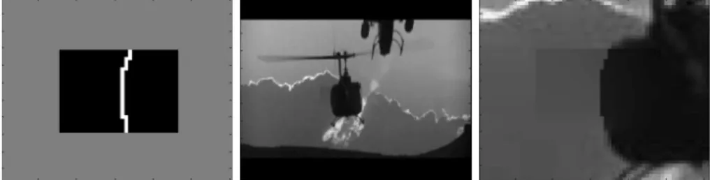
We now consider another application of this technique to image inpainting and improve the results presented in [2]. The idea of the topological gradient algo-rithm is to identify the missing edges in the occluded part of the image, and then to reconstruct the image from the solution of a Poisson problem with Neumann boundary conditions (see references in [2]). In this application also, it is crucial to have connected contours, otherwise the reconstruction with the Laplacian will not be satisfactory. Figure 4 shows an example of image, in which we added a mask on a quite large part of the image (≃ 800 pixels). The goal of inpainting is to reconstruct as precisely as possible the original image from the occluded im-age. We also want the inpainted image to have sharp (unblurred) edges. Figure 4 shows the corresponding topological gradient, provided by the inpainting algo-rithm (see [2] for more details about this algoalgo-rithm). In this case, the topological gradient gives some information about the most probable location of the missing edges. In [2], the idea is then to threshold the topological gradient, and define the edge set of the occluded zone as being the set of points below the threshold. The main issue is that the identified missing edges must be connected in order to avoid blurry effects (due to the Laplacian) in the reconstruction. Then, the threshold is sometimes set manually in order to have connected contours. In our example, the identified edge set is represented by white points in figure 4.
Figure 4 shows the corresponding inpainted image. One can see that the reconstruction is not very good, particularly in the top part. This is mainly due to the fact that the identified edges are either connected but thick with a lot of wrong identifications (if the threshold is too small) or discontinuous (otherwise).
Fig. 4.Top: Occluded image (by a white rectangle) (left); zoom of the occluded zone and topological gradient (right); Bottom: Inpainted image using the edge set from the topological gradient and zoom of the occluded zone, and edge set (right).
Fig. 5. Admissible set of keypoints (left); selected keypoints on the topological gra-dient and minimal path between the keypoints represented on the occluded image as corresponding identified missing edge (right).
The idea of our method is to apply the fast marching algorithm on the topological gradient obtained during the inpainting process, in order to identify connected contours in the hidden part of the image.
After thresholding the topological gradient, several points (identified by blue circles) have been identified and define the admissible set of keypoints, repre-sented in figure 5-left. We choose then the most negative point of the topological gradient as the first keypoint, and then the further admissible point as the sec-ond one. The keypoints are represented by a large black point on the same image. They are located on the edge of the domain, as the inpainting topological gradient always takes its minimal values there.
Then the minimal path algorithm is run, and it provides a path between the keypoints, represented in green in figure 5-right. We can see that the path follows very well the valley line of the topological gradient, from one side to the other. By choosing 3 keypoints instead of 2, there will be another keypoint on the bottom edge, near the first one, and it will simply add a small contour
Fig. 6. Inpainted image using the fast marching algorithm for closing the contours identified by the topological gradient in the hidden part of the image, and corresponding zoom.
located all along on the edge of the domain, and consequently there is absolutely no impact on the reconstruction of the hidden part of the image.
Figure 5 shows on the right the same identified path represented on the occluded image. This allows one to see that the path clearly gives a good ap-proximation of the missing edges, and also that the topological gradient is very powerful for this identification problem. The corresponding identified edge set is represented in figure 6-left. This image should be compared with the thresholded edge set of figure 4-right. And we can conclude that the minimal path algorithm is an excellent tool for extracting the valley lines of the topological gradient.
Finally, using this minimal path as the set of missing edges in the occluded zone, the inpainting topological gradient algorithm produces a much better re-constructed image, shown in figure 6. The quality of the image is very good, as the missing edges used for the reconstruction are connected, and the Laplace operator will not produce any blurring effect due to a discontinuous contour. This example confirms that the quality of all topological gradient applications in image processing can be improved, by replacing a thresholding technique by a minimal path algorithm.
4
Conclusions and perspectives
We have introduced a hybrid scheme, based on one side on the topological gradi-ent for edge detection, and on the other side on the fast marching and minimal paths methods for contour completion. These approaches allow us to extract connected contours in 2D images, and to solve the main issue of all topological gradient based algorithms for image processing problems (discontinuity of the edges). Moreover, the minimal path algorithm does not degrade the complexity of the topological asymptotic analysis.
We have considered two specific applications in image processing: segmenta-tion and inpainting. In the first one (segmentasegmenta-tion), we showed that the topolog-ical gradient is more efficient than the standard gradient for edge detection, and the hybrid scheme provides better results than the fast marching method applied to the standard gradient of the image. In the second application (inpainting), we
showed that the hybrid scheme particularly improves the quality of the inpainted image, as the contour completion ensures a non-blurred inpainted image, and as it also helps removing the manual thresholding of the topological gradient.
An interesting and natural perspective is to apply this hybrid scheme to 3D images and movies. The topological gradient can very easily be extended to 3D images as well as the minimal path technique.
References
[1] Ardon, R., Cohen, L.D., Yezzi, A.: A new implicit method for surface segmentation by minimal paths in 3D images. Applied Mathematics and Optimization 55(2), 127–144 (March 2007)
[2] Auroux, D., Masmoudi, M.: Image processing by topological asymptotic expan-sion. J. Math. Imaging Vision 33(2), 122–134 (2009)
[3] Chan, T., Shen, J.: Non-texture inpainting by curvature-driven diffusions (CDD). Tech. Rep. 00-35, UCLA CAM (September 2000)
[4] Cohen, L.D.: Minimal paths and fast marching methods for image analysis. Math-ematical models in computer vision: the handbook, N. Paragios, Y. Chen and O. Faugeras (Eds), Springer (2005)
[5] Cohen, L.D.: Multiple contour finding and perceptual grouping using minimal paths. J. Math. Imaging Vision 14(3), 225–236 (2001)
[6] Dicker, J.: Fast marching methods and level set methods: an implementation. Ph.D. thesis, University of British Columbia (2006)
[7] Elad, M., Starck, J.L., Querre, P., Donoho, D.L.: Simultaneous cartoon and tex-ture image inpainting using morphological component analysis (MCA). J. Appl. Comput. Harmonic Anal. 19, 340–358 (2005)
[8] Jaafar-Belaid, L., Jaoua, M., Masmoudi, M., Siala, L.: Image restoration and edge detection by topological asymptotic expansion. C. R. Acad. Sci., Ser. I 342(5), 313–318 (2006)
[9] Masmoudi, M.: The topological asymptotic, Computational Methods for Control Applications, R. Glowinski, H. Karawada, and J. P´eriaux (Eds.), vol. 16, pp. 53–72. GAKUTO Internat. Ser. Math. Sci. Appl., Tokyo, Japan (2001)
[10] Rawlinson, N., Sambridge, M.: The fast marching method: an effective tool for tomographic imaging and tracking multiple phases in complex layered media. Explor. Geophys. 36, 341–350 (2005)
[11] Sethian, J.A.: Level set methods and fast marching methods. Cambridge Univer-sity Press (1999)
[12] Telea, A., van Wijk, J.: An augmented fast marching method for computing skele-tons and centerlines. In: Proc. Eurographics IEEE-TCVG Symposium on Visual-ization. Springer, Vienna (2002)
[13] Wen, P., Wu, X., Wu, C.: An interactive image inpainting method based on rbf networks. In: 3rd Int. Symposium on Neural Networks. pp. 629–637 (2006) [14] Zhou, T., Tang, F., Wang, J., Wang, Z., Peng, Q.: Digital image inpainting with
radial basis functions. J. Image Graphics (In Chinese) 9(10), 1190–1196 (2004) [15] Zhu, F., Tian, J.: Modified fast marching methods and level set method for medical