HAL Id: hal-01945320
https://hal.inria.fr/hal-01945320
Submitted on 5 Dec 2018
HAL is a multi-disciplinary open access
archive for the deposit and dissemination of
sci-entific research documents, whether they are
pub-lished or not. The documents may come from
teaching and research institutions in France or
abroad, or from public or private research centers.
L’archive ouverte pluridisciplinaire HAL, est
destinée au dépôt et à la diffusion de documents
scientifiques de niveau recherche, publiés ou non,
émanant des établissements d’enseignement et de
recherche français ou étrangers, des laboratoires
publics ou privés.
Bryan Pardo, Antoine Liutkus, Zhiyao Duan, Gael Richard
To cite this version:
Bryan Pardo, Antoine Liutkus, Zhiyao Duan, Gael Richard. Applying source separation to music.
Audio Source Separation and Speech Enhancement, Chapter 16, Wiley, 2018, 978-1-119-27989-1.
�10.1002/9781119279860.ch16�. �hal-01945320�
1
Applying source separation to music
Bryan Pardo, Antoine Liutkus, Zhiyao Duan, Gaël RichardSeparation of existing audio into re-mixable elements is useful in many contexts, especially in the realm of music and video remixing. Much musical audio content, including audio tracks for video, is available only in mono (e.g. 1940’s movies and records) or 2-channel stereo (YouTube videos, commercially released music where the source tracks are not available). Separated sources from such tracks would be useful to repurpose this audio content. Applications include upmixing video sound-tracks to surround sound (e.g. home theater 5.1 systems), facilitating music transcrip-tion by separating into individual instrumental tracks, allowing better mashups and remixes for DJs, and rebalancing sound levels after multiple instruments or voices were recorded simultaneously to a single track (e.g. turning up only the dialog in the movie, not the music). Effective separation would also let producers edit out in-dividual musician’s note errors in a live recordings without need for an inin-dividual microphone on each musician, or apply audio effects (equalization, reverberation) to individual instruments recorded on the same track. Given the large number of poten-tial applications and their impact, it is no surprise that many researchers have focused on the application areas of music recordings and movie soundtracks. In this chap-ter, we provide an overview of the algorithms and approaches designed to address the challenges and opportunities in music. Where applicable, we will also introduce commonalities and links to source separation for video soundtracks, since many mu-sical scenarios involve video soundtracks (e.g. YouTube recordings of live concerts, movie sound tracks).
1.1
Challenges and opportunities
Music, in particular, provides a unique set of challenges and opportunities that have led algorithm designers to create methods particular to the task of separating out elements of a musical scene.
1.1.1
Challenges
In many non-musical scenarios (e.g. recordings in a crowded street, multiple conver-sations in a cocktail party) sound sources are uncorrelated in their behavior and have relatively little overlap in time and frequency. In music, sources are often strongly correlated in onset and offset times, such as a choir singing together. This kind of correlation makes approaches that depend on independent component analysis un-reliable. Sources also often have strong frequency overlap. For example, voices singing in unison, octaves, or fifths produce many harmonics that overlap in fre-quency. Therefore, time-frequency overlap is a significant issue in music.
Unrealistic mixing scenarios are also common in both music and commercial videos. Both music and video sound tracks are often recorded in individual tracks that have individual equalization, panning and reverberation applied to each track prior to the mixdown. Therefore, systems that depend on the assumption that sources share a reverberant space and have self-consistent timing and phase cues resulting from placement in a real environment will encounter problems.
These problems can be exacerbated in pop music, where it may be difficult to say what constitutes a source, as the sound may never have been a real physical source, such as the output of a music synthesizer. A single sonic element may be composed of one or more recordings of other sources that have been manipulated and layered together (e.g. drum loops with effects applied to them, or a voice with pre-verb and octave doubling applied to it).
Finally, evaluation criteria for music are different than for problems such as speech separation. Often, intelligibility is the standard for speech. For music, it is often an artistic matter. For some applications the standard may be that a separated source must sound perfect, while for others, perhaps the separation need not be perfect, if the goal is to simply modify the relative loudness of a source within the mixture. Therefore, the choice of an evaluation measure is more task dependent than for some other applications.
1.1.2
Opportunities
Music also provides opportunities that can be exploited by source separation algo-rithms. Music that has a fully-notated score provides knowledge of the relative timing and fundamental frequency of events. This can be exploited to inform source sepa-ration (e.g. seeding the activation and matrix and spectral templates in NMF (Ewert and Muller, 2012)) Acoustic music typically has a finite set of likely sound-producing sources (e.g. a string quartet almost always has two violins, one viola and one cello). This provides an opportunity to seed source models with timbre information, such as from libraries of sampled instrument sounds (Rodriguez-Serrano et al., 2015a). Even when a score or list of instruments is not available, knowledge of musical rules can be used to construct a language model to constrain likely note transitions. Com-mon sound engineering (Ballou, 2013) and panning techniques can be used to
per-form vocal isolation on many music recordings. For example, vocals are frequently center-panned. One can retrieve the center panned elements of a 2-channel recording by phase inverting the left channel and subtracting it from the right channel.
Often, the musical structure, itself, can be used to guide separation, as composers frequently group elements working together and present them in ways to teach the lis-tener what the important groupings are. This can be used to guide source separation (Seetharaman and Pardo, 2016). If the goal is to separate the background music from the speech in a recording, having multiple examples of the recording, with different speech is very helpful. This is often possible with music concert recordings and with commercially released video. It is common for multiple people to record the same musical performance (e.g. YouTube concert videos). This can often provide multiple channels that allow a high-quality audio recording to be constructed from multiple low-quality ones (Kim and Smaragdis, 2013). Commercially released video content that has been dubbed into multiple languages provides a similar opportunity.
Having laid out the challenges and opportunities inherent in musical source sepa-ration, we now move on to discuss the ways that source separation techniques have been adapted to or designed for separation of music. We begin with non-negative matrix factorization (NMF).
1.2
Nonnegative matrix factorization in the case of music
The previous chapters have already included much discussion on NMF and its use in audio source separation, particularly in the case of speech. NMF has been widely used for music source separation since it was introduced to the musical context in 2003 (Smaragdis and Brown, 2003). The characteristics of music signals have called for dedicated models and numerous developments and extension of the basic "blind" NMF decomposition. In this section, we discuss some of the extension of the models described in Chapters ?? and ?? for the particular case of music signals.
1.2.1
Shift-invariant NMF
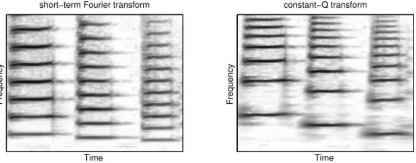
While the relative strengths of harmonics in vocals are constantly changing, many musical instruments (e.g. flutes, saxophones, pianos) produce a harmonic overtone series that keeps relationships relatively constant between the amplitudes of the har-monics even as the fundamental frequency changes. This shift-invariance is made clear when the audio is represented using the log of the frequency, rather than repre-senting frequency linearly, as the widely-used short time Fourier transform (STFT) does. Therefore, many instruments may well be approximated as frequency shift in-variant in a log-frequency representation, such as the constant-Q transform (CQT) (Brown, 1991). The CQT allows one to represent the signal with a single frequency pattern, shifted in frequency for different pitches. This is illustrated in Fig. 1.1 on a musical signal composed of three successive musical notes of different pitch. With
the STFT, these three notes would need at least three frequency patterns to represent them.
short−term Fourier transform
Time
Frequency
constant−Q transform
Time
Frequency
Figure 1.1 Comparing short-term Fourier transform (STFT) and constant-Q transform
(CQT) representation on a trumpet signal composed of three musical notes of different pitch.
Based on such a log-frequency transformation, several shift-invariant approaches have been proposed for audio signal analysis, especially in the framework of prob-abilistic latent component analysis (PLCA), the probprob-abilistic counterpart of NMF (Smaragdis et al., 2008). An extension of the initial framework, called blind har-monic adaptive decomposition (BHAD) was presented by Fuentes et al. (2012) to better model real music signals. In this model, each musical note may present fun-damental frequency and spectral envelope variations across repetitions. These char-acteristics make the model particularly efficient for real musical signals.
More precisely, the absolute value of the normalized CQT representation is mod-eled as the sum of an harmonic component and a noise component. The polyphonic harmonic component is modeled as a weighted sum of different harmonic spectra (to account for harmonics from multiple sources), each one having its own spectral envelope and pitch. One can notice thanks to the CQT properties, a pitch modulation can be seen as a frequency shifting of the partials that can be exploited in the model. Concurrently, the noise component is modeled as the convolution of a fixed smooth narrow-band frequency window and a noise time-frequency distribution.
The original approach is entirely unsupervised as most other approaches in this framework, which rely on prior generic information or signal models to obtain a semantically meaningful decomposition. It was shown in some controlled cases that improved performance can be obtained by integrating a learning stage or by adapting the pre-learned models using a multi-stage transcription strategy (see Benetos et al. (2014) for example) or by involving a user during the transcription process (Kirchhoff
et al., 2013; Bryan et al., 2013). It was in particular shown by de Andrade Scatolini et al.(2015) that a partial annotation brings further improvement by providing a better
1.2.2
Constrained and structured NMF
The success of NMF for music source separation is largely due to its flexibility to take advantage of important characteristics of music signals in the decomposition. Indeed, those characteristics can be used to adequately constrain the NMF decomposition. Numerous extensions have then been proposed to adapt the basic "blind" NMF model to incorporate constraints or data source structures (see Chapters ?? and ??, as well as Wang and Zhang (2013)). In this section, we will only focus on some extensions that are specific to the case of music signals namely to the incorporation of constraints deduced from music instrument models or from general music signal properties.
Exploiting music instrument models
In acoustic music, the individual sources are typically produced by acoustic music instruments whose physical properties can be learned or modeled. We illustrate be-low three instrument models that have been successfully applied to NMF for music source separation.
• Harmonic and inharmonic models in NMF: a large set of acoustic music instru-ments produce well defined pitches composed of partials or tones in relatively pure harmonic relations. For some other instruments, such as piano for example, due to the string stiffness, the frequencies of the partials slightly deviate from a purely harmonic relationships. Depending on the type of music signals at hand, specific parametric models can be built and used in NMF decompositions to model the spectra of the dictionary atoms. Harmonic models have been exploited in multi-ple works (Hennequin et al., 2010; Bertin et al., 2010). As an extension of this idea, Rigaud et al. (2013) proposed an additive model for which three different constraints on the partial frequencies were introduced to obtain a blend between a strict harmonic and a strict inharmonic relation given by specific physical models. • Temporal evolution models in NMF: The standard NMF is shown to be efficient when the elementary components (notes) of the analyzed music signal are nearly stationary. However, in several situations, elementary components can be strongly non stationary and the decomposition will need multiple basis templates to repre-sent a single note. Incorporating temporal evolution models in NMF is then partic-ularly attractive to represent each elementary component with a minimal number of basis spectra. Several models were proposed including the Auto-Regressive Mov-ing Average (ARMA) time varyMov-ing model introduced by Hennequin et al. (2011) to constrain the activation coefficients which allowed to obtain an efficient single-atom decomposition for a single audio event with strong spectral variations. An-other strategy to better model the temporal structure of sounds is to rely on hidden Markov models (HMM) that aim at describing the structure of changes between subsequent templates or dictionaries used in the decomposition (Mysore et al., 2010).
• Source-filter models in NMF: Some instruments such as the singing voice are well represented by a source-filter production model with negligible interaction
be-tween the source (e.g. the vocal cords) and the filter (e.g. the vocal tract). Using such a production model has several advantages. First, it adds meaningful con-straints to the decomposition which help to converge to an efficient separation. Second, it allows to choose appropriate initializations for example by pre-defining acceptable shapes for source and filter spectra. Third, it avoids the usual permu-tation problem of frequency-domain source separation methods since the com-ponent obeying to the source-filter model is well identified. This motivated the use of source filter models in music source separation for singing voice extraction (Durrieu et al., 2011, 2010) but also for other music instruments (Heittola et al., 2009). Durrieu et al. (2011) model the singing voice by a specific NMF source-filter model and the background by a regular and unconstrained NMF model as expressed below: |X|2≈ WF | {z } Filter WF0 | {z } Source + BMHM | {z } Background
with |X|2denoting element-wise exponentiation and where BM is the dictionary
and HM the activation matrices of the NMF decomposition1)of the background component and where WF(respectively WF0) represents the filter part (resp. the
source part) of the singing voice component. Both the filter and source parts are further parameterized to allow good model expressivity . In particular, the filter is defined as a weighted combination of basic filter shapes, themselves built as a a linear weighted combination of atomic elements ( for example, a single resonator symbolizing a formant filter). The filter part is then given by:
WF = BFHFHΦ
where BF gathers the filter atomic elements, HF the weighting coefficients of
the filter atomic elements to build basic filter shapes and HΦthe weighting
co-efficients of the basic filter shapes. Concurrently, the source part is modeled as a positive linear combination of a number (in the ideal case reduced to one) of fre-quency patterns which represent basic source power spectra obtained by a source production model. The source part is then expressed as:
WF0= BF0HF0
where BF0 gathers the basic source power spectra for a predefined range of
fun-damental frequencies F0and HF0the weighting (or activation) coefficients. Exploiting music signal models
Another strategy for adapting the raw NMF decompositions to music signals is to rely on dedicated signal models. Contrary to the music instrument models described above, these models are more generic and generally apply to a large class of music signals. Two examples of such signal models are briefly described below.
• Harmonic/percussive models in NMF: In general, harmonic instruments tend to produce few tones simultaneously which are slowly varying in times. Enforcing temporal smoothness and sparsity of the decomposition is therefore an efficient strategy for separating harmonic instruments (Virtanen, 2007). Recently, Canadas-Quesada et al. (2014) use four constraints to achieve a specific harmonic/percussive decomposition with NMF. An alternative strategy is to rely on specific decomposi-tion models that will automatically highlight the underlying harmonic/percussive musical concepts. Orthogonal NMF and projective NMF (PNMF) (Choi, 2008) are typical examples of such decompositions. For example, Laroche et al. (2015) used PNMF to obtain an initial nearly-orthogonal decomposition well adapted to represent harmonic instruments. This decomposition is further extended by a non-orthogonal component that reveals to be particularly relevant to represent percus-sive or transient signals. The so-called structured projective NMF (SPNMF) model is then given by:
|X|2≈ BhHh | {z } Harmonic + BpHp | {z } Percussive
where Bh (resp. Bp) gathers the harmonic (resp. percussive) atoms and Hh
(resp. Hp) the activation coefficients of the harmonic (resp. percussive)
compo-nent. Note that in this model, the harmonic part is obtained by PNMF and the percussive part by a regular NMF.
• Musical constraints in NMF models: To adapt the decomposition to music signals, it is also possible to integrate constraints deduced from high level musical concepts such as temporal evolution of sounds, rhythm structure or timbral similarity. For example, Nakano et al. (2010, 2011) constrain the model by using a Markov chain that governs the order in which the basis spectra appear for the representation of a musical note. This concept is extended by Kameoka et al. (2012) where a beat-structure constraint is included in the NMF model. This constraint allowed to better represent the different note onsets. It is also possible to rely on timbre similarity for grouping similar spectra which shall describe the same instrument (e.g. the same source). An appropriate grouping of basis spectra allows one to improve the decomposition of each source since more basis spectra can be used without spreading an original source in several separated estimates as in unconstrained NMF.
When additional information is available (such as the score), it is possible to use better musical constraints as further discussed in Section 1.3.3. It is also worth men-tioning that a number of applications may benefit from a two component model such as the one briefly sketch for singing voice separation or harmonic/percussive decom-position (see for example Section 1.5.1 in the context of movie content remastering using multiple recordings).
1.3
Taking advantage of the harmonic structure of music
Harmonic sound sources (e.g., strings, woodwind, brass and vocals) are widely present in music signals and movie sound tracks. The spectrum of a harmonic sound source shows a harmonic structure: prominent spectral components are located at integer multiples of the fundamental frequency of the signal and hence are called
harmonics; relative amplitudes of the harmonics are related to the spectral
enve-lope and affect the timbre of the source. Modeling the harmonic structure helps to organize the frequency components of a harmonic source and separate it from the mixture.
1.3.1
Pitch-based Harmonic Source Separation
The most intuitive idea for taking advantage of the harmonic structure is to organize and separate spectral components of a harmonic source according to its fundamental frequency (F0), which is also referred as the pitch. Estimating the concurrent F0s from a mixture of harmonic sources in each time frame, i.e., multi-pitch estimation (MPE), is thus the first important step. MPE is a challenging research problem on its own, and many different approaches have been proposed. Time-domain approaches try to estimate the period of harmonic sources using autocorrelation functions (Tolo-nen and Karjalai(Tolo-nen, 2000) or probabilistic sinusoidal modeling (Davy et al., 2006). Frequency-domain approaches attempt to model the frequency regularity of harmon-ics (Klapuri, 2003; Duan et al., 2010). Spectrogram decomposition methods use fixed (Ari et al., 2012) or adaptive (Bertin et al., 2010) harmonic templates to rec-ognize the harmonic structure of harmonic sources. There are also approaches that fuse time-domain and frequency-domain information towards MPE (Su and Yang, 2015).
With the fundamental frequency of a harmonic source estimated in a time frame, a harmonic mask can be constructed to separate the source from the mixture. This mask can be binary so that all the spectral energy located at the harmonic frequen-cies is extracted for the source (Li and Wang, 2008). However, when harmonics of different sources overlap, a soft mask is needed to allocate the mixture signal’s spec-tral energy to these overlapping sources appropriately. This overlapping harmonic issue is very common in music signals. This is due to the fact that tonal harmony composition rules prefer small integer ratios among the F0s of concurrent harmonic sources. For example, the frequency ratios of the F0s of a C major chord is C:E:G = 4:5:6. This causes 46.7% of the harmonics of the C note, 33.3% of E and 60% of G, being overlapped with the other two notes.
A harmonic index is the integer multiple that one must apply to the fundamental frequency (F0) to give the frequency of a harmonic. One simple, effective method to allocate the spectral energy to overlapping harmonics is to consider the harmonic indexes. Higher harmonics tend to be softer than lower harmonics for most harmonic sounds. Therefore, the spectral energy tends to decrease when the harmonic index
increases. Thus, it is reasonable to allocate more energy to the source whose low-indexed harmonic is overlapped by a higher-low-indexed harmonic of another source. Duan and Pardo (2011b) proposed to build a soft mask on the magnitude spectrum inverse proportional to the square of the harmonic index:
mi= 1/h2 i ΣJ j=11/h2j (1.1) where miis the mask value for the i-th source at the overlapping harmonic frequency
bins; hkis the harmonic index of the k-th source. This is based on the assumption
that 1) overlapping sources have roughly the same energy, and 2) the spectral energy decays at a rate of 12 dB per octave regardless the pitch and instrument. Although this simple method achieves descent result, the assumptions are obviously oversimplified. For example, it does not model the timbre of the sources, which we will discuss in the next section.
1.3.2
Modeling Timbre
Multi-pitch estimation and harmonic masking allows us to separate harmonic sources in each individual frame. However, how can we organize the sources over time? In other words, which pitch (and its harmonics) belongs to which source? In auditory scene analysis (Bregman, 1994), this is called sequential grouping, or streaming. Commonly used grouping cues include time and frequency proximity (i.e., sounds that are close in both time and frequency are likely to belong to the same source) and timbre and location consistency (i.e., sounds from the same source tend to have similar timbre and location while sounds from different sources often have distinct timbre and location). Time and frequency proximity cues, however, only help to group pitches within the same note, because there is often a gap in time and/or fre-quency between two successive notes from the same source. In addition, the location consistency cue can only be exploited in stereo or multi-channel recordings, where the Inter-channel Intensity Difference (IID) and Inter-channel Time Difference (ITD) can be calculated to localize sound sources. The timbre consistency cue, on the other hand, is more universal.
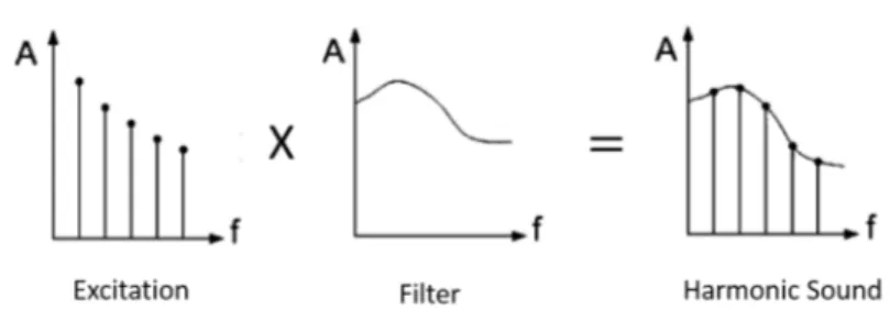
One widely adopted approach to dis-entangle pitch and timbre of a harmonic sound is the source-filter model. It is also called the excitation-resonance model. As shown in Figure 1.2, a harmonic sound, such as one produced by a clarinet, can be modeled as the convolution of an excitation signal (vibration of the clarinet reed) with a filter’s impulse response (determined by the clarinet body). In the frequency domain, the magnitude spectrum of the harmonic sound is then the multiplication of the mag-nitude spectrum of the excitation signal and that of the filter’s frequency response. The excitation spectrum is often modeled as a harmonic comb with flat or decaying amplitudes; it determines the F0 and harmonic frequencies. The filter’s frequency response, on the other hand, characterizes the slowly varying envelope of the signal’s spectrum; it is considered to affect the timbre of the signal.
Figure 1.2 The source-filter model in the magnitude frequency domain.
Various ways for representing the spectral envelope have been proposed. Mel-frequency Cepstral Coefficients (MFCC) (Davis and Mermelstein, 1980) are a com-monly used representation. However, MFCCs must be calculated from the full trum of a signal. Therefore, this representation cannot be used to represent the spec-tral envelope of a single source, if the source has not been separated from the mix-ture. It is reasonable, though, to assume that some subset of the desired source’s spectrum is not obscured by other sources in the mixture. This subset can be sparse in frequency and the spectral values can be noisy. For example, with the F0 of a source being estimated, the spectral points at the harmonic positions are likely to belong to the source spectrum, although the spectral values can be contaminated by the overlapping harmonics. Based on this observation, timbre representations that can be calculated from isolated spectral points have been proposed, such as the dis-crete cepstrum (Galas and Rodet, 1990), regularized disdis-crete cepstrum (Cappé et al., 1995), and uniform discrete cepstrum (UDC) (Duan et al., 2014b). UDC and its mel-frequency variant MUDC have been shown to achieve good results in instru-ment recognition in polyphonic music mixtures as well as multi-pitch streaming in speech mixtures (Duan et al., 2014a).
Another timbre representation that does not directly characterize the spectral enve-lope but can be calculated from harmonics is the harmonic structure feature. It is de-fined as the relative logarithmic amplitude of harmonics (Duan et al., 2008). Within a narrow pitch range (e.g., two octaves), the harmonic structure feature of musical instruments has been shown to be quite invariant to pitch and dynamic and also quite discriminative among different instruments. Based on this observation, Duan et al. (2008) proposed an unsupervised music source separation method that clusters the harmonic structure features of all pitches detected in a piece of music. Each cluster corresponds to one instrumental source and the average of the harmonic structures within the cluster is calculated and defined as the Average Harmonic Structure (AHS) model. Sound sources are then separated using the AHS models.
Duan et al. (2014a) further pursued the clustering idea by incorporating pitch lo-cality constraints into the clustering process. A must-link constraint is imposed be-tween two pitches that are close in both time and frequency to encourage them to be assigned to the same cluster. A cannot-link constraint is imposed between si-multaneous pitches to encourage them to be assigned to different clusters, under the
assumption of monophonic sound sources. These constraints implement the time and frequency proximity cue in auditory scene analysis. With these constraints, the clustering problem becomes a constrained clustering problem. A greedy algorithm is proposed to solve this problem and is shown to achieve good results in multi-pitch streaming for both music and speech sound mixtures. Although this method was de-signed to address multi-pitch streaming instead of source separation, sound sources can be separated by harmonic masking on the pitch streams as discussed in Section 1.3.1.
This constrained clustering idea has also been pursued by others. Arora and Be-hera (2015) designed a Hidden Markov Random Field (HMRF) framework for multi-pitch streaming and source separation of music signals. Timbre similarity between pitches is defined as the HMRF likelihood and pitch locality constraints are defined as HMRF priors. MFCCs of the separated spectrum of each pitch is used as the tim-bre representation. Hu and Wang (2013) proposed an approach to cluster TF units according to their Gammatone Frequency Cepstral Coefficients (GFCC) features for speech separation of two simultaneous talkers.
1.3.3
Training and Adapting Timbre Models
When isolated training recordings of the sound sources are available, one can train timbre models beforehand and then apply these models to separate sources from the audio mixture. Various NMF-based source separation approaches rely on this as-sumption (Smaragdis et al., 2007) (see Section 1.2 for various kinds of NMF mod-els). To take advantage of the harmonic structure of musical signals, the dictionary templates (basis spectra) can be designed as harmonic combs to correspond to the quantized musical pitches (Bay et al., 2012) whose amplitudes are learned from train-ing materials. To account for minor pitch variations such as vibrato, shift-invariant NMF has been proposed to shift the basis spectra along the frequency axis (see Sec-tion 1.2.1). When the shift invariance is used at its maximum strength, different pitches of the same instrument are assumed to share the same basis spectrum as in (Kim and Choi, 2006). This is similar to the harmonic structure idea in Section 1.3.2. This significantly reduces the number of parameters in the timbre models, however, the shift invariance assumption is only valid within a narrow pitch range.
Another way to reduce the number of parameters in the pitch-dependent NMF dic-tionaries is to adopt a source-filter model (Section 1.2.2 describes source filter models in the context of NMF). The simplest approach is to model each basis function as the product of a pitch-dependent excitation spectrum and an instrument-dependent filter as in (Virtanen and Klapuri, 2006). This model can be further simplified to make the excitation spectrum always be a flat harmonic comb as in (Klapuri et al., 2010). This simple model is able to represent some instruments with a smooth envelope of their spectral peaks. However, the spectral envelope of other instruments, such as the clarinet, are not smooth and they cannot be well represented with a flat excitation function. For example, the second harmonic of a clarinet note is often very soft, no matter what pitch the note has. This makes it impossible to represent the spectral
envelopes of different clarinet notes with a single filter.
To deal with this issue, Carabias-Orti et al. (2011) proposed a Multi-Excitation per Instrument (MEI) model. This model defines the excitation spectrum of each pitch as a linear combination of a few pitch-independent excitation basis vectors with pitch-dependent weights. The excitation basis vectors are instrument dependent but are not pitch dependent. The weights in the linear combination, however, are both instrument dependent and pitch dependent. This MEI model is a good comprise between the regular source filter model and the flat harmonic comb model. Compared to the regular source-filter model, the MEI model significantly reduces the number of parameters. Compared to the flat harmonic comb model, the MEI model preserves the flexibility of modeling sources whose excitation spectra are not flat, such as the clarinet.
To adapt the pre-learned timbre models to the sources in the music mixture, the source dictionaries can be first initialized with the pre-learned dictionaries, and then kept updating during the separation process such as in (Ewert and Muller, 2012). This approach, however, only works well when the initialization is very good or strong constraints of the dictionary and/or the activation coefficients are imposed (e.g., score-informed constraints in Section 1.3.4). Another way is to set the pre-learned dictionary as a prior (e.g., Dirichlet prior) of the source dictionary (Rodriguez-Serrano et al., 2015a). In this way, the updating of the source dictio-naries can be guided by the pre-learned models throughout the separation process, hence is more robust when strong constraints are not available.
1.3.4
Score-informed Source Separation
When available, the musical score can significantly help music source separation (Ewert et al., 2014), First, it helps pitch estimation, based on which harmonics of the sound source can be organized in each frame. Second, it helps note activity detection, which is especially important for NMF-based approaches. Third, it helps to stream pitches of the same source across time, which is a key step for pitch-based source separation.
To utilize the score information, audio-score alignment is needed to synchronize the audio with the score. Various approaches for polyphonic audio-score alignment has been proposed. There are two key components of audio-score alignment: the feature representation and the alignment method. Commonly used feature represen-tations include the chromagram (Fujishima, 1999), multi-pitch represenrepresen-tations (Duan and Pardo, 2011a), and auditory filter bank responses (Montecchio and Orio, 2009). Commonly used alignment methods include Dynamic Time Warping (DTW) (Orio and Schwarz, 2001), Hidden Markov Models (HMM) (Duan and Pardo, 2011a), and Conditional Random Fields (CRF) (Joder and Schuller, 2013). Audio-score align-ment can be performed offline or online. Offline methods require the access of the entire audio recording beforehand, while online methods do not need to access fu-ture frames when aligning the current frame. Therefore, offline methods are often more robust while online methods are suitable for real-time applications including
real-time score-informed source separation (Duan and Pardo, 2011b).
Once the audio and score are synchronized, the score provides information about what notes are supposed to be played in each audio frame by each source. This information is very helpful for pitch estimation. In (Duan and Pardo, 2011b), the actually performed audio pitches are estimated within one semitone of the score-indicated pitches. This significantly improves the MPE accuracy, which is essential for pitch-based source separation. Finally, harmonic masking is employed to sepa-rate the signal of each source. Rodriguez-Serrano et al. (2015b) further improved this approach by replacing harmonic masking with a multi-excitation per instrument (MEI) source-filter NMF model to adapt pre-learned timbre models for the sources in the mixture. Ewert and Muller (2012) proposed to employ the score information through constraints for an NMF-based source separation model to separate sounds played by the two hands in a piano recording. The basis spectra are constrained to be harmonic combs where values outside a frequency range of each nominal musical pitch are set to zero. The activation coefficients of the basis spectra are set according to the note activities in the score. Values outside a time range of the note duration are set to zero. As the multiplicative update rule is used in the NMF algorithm, zero values in the basis spectra or the activation coefficients will not be updated. There-fore, this initialization imposes strong constraints that are informed by the score on the NMF update process.
1.4
Nonparametric local models: taking advantage of redundancies in music
As we have seen above, music signals come with a particular structure that may be exploited to constraint separation algorithms for better performance. In the previous section, we discussed an approach where separation models are described explicitly with two main ingredients. The first one is a musicologically meaningful informa-tion, the score, that indicates which sounds are to be expected at each time instant. The second one is a parametric signal model that describes each sound independently of when it is activated in the track. For this purpose, we considered harmonic and NMF models.
Apart from their good performance when correctly estimated, the obvious advan-tage of such parametric models for music separation is their interpretability. They make it possible to help the algorithm with specific high-level information such as the score or user input, as we will see shortly.
However, explicit parameterization of the musical piece using a multi-level ap-proach is sometimes not the most natural nor the most efficient solution. Its most de-manding constraint, which is critical for good performance, is that the superimposed signals obey their parametric models. While this may be verified in some cases, it may also fail in others, especially for sources found in real full-length popular songs. A first option to address this issue may be to use more realistic acoustic models such as Deep Neural Networks (DNN) instead of NMF, but this comes with the need of gathering a whole development database to learn them.
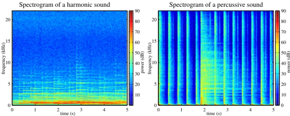
time (s) freq uency (kHz) 0 1 2 3 4 5 0 5 10 15 20 po w er (dB ) 10 20 30 40 50 60 70 80 90 time (s) freq uency (kHz) 0 1 2 3 4 5 0 5 10 15 20 po w er (dB ) 0 10 20 30 40 50 60 70 80 90
Figure 1.3 Local regularities in the spectrograms of percussive (vertical) and harmonic
(horizontal) sounds
An alternative option we present in this section is to avoid explicit parameteri-zation of the Power Spectral Density (PSD) of each source but rather to focus on a non-parametric approach that exploits only its local regularities. This track of research leads to numerous efficient algorithms such as HPSS (Fitzgerald, 2010), REPET (Rafii and Pardo, 2011, 2013; Liutkus et al., 2012) or KAM (Liutkus et al., 2014), that we discuss now.
1.4.1
HPSS: Harmonic-Percussive Source Separation
As an introductory example for non-parametric audio modeling, consider again the scenario where we want to separate the drums section of a music piece that was mentioned in section 1.2.2 above. This can happen, for instance, when a musician wants to reuse some drum loops to mix them with another instrumental accompa-niment. We already discussed parametric approaches where both the drum signal and the harmonic accompaniment would be described explicitly through particular spectral templates or the smoothness of their activation parameters, or thanks to their score. However, a very different approach considered in (Fitzgerald, 2010) directly concentrates on the raw spectrograms of these different sources and uses a simple fact: drum sounds tend to be located in time (percussive), while the accompaniment is rather composed of very narrowband sinusoidal partials located in frequency (har-monic). As an example, consider the two spectrograms on figure 1.3. We can see that both percussive and harmonic sounds are characterized by vertical or horizon-tal lines in their spectrograms. Given a music signal, we may hence safely assume that the vertical lines in its spectrogram are mostly due to drums sound, while the horizontal ones pertain to accompaniment.
This simple idea leads to the celebrated HPSS algorithm (Fitzgerald, 2010): given a mixture spectrogram |X|, we apply a median filter on it along the time (resp. fre-quency) dimension to keep only the harmonic (resp. percussive) contribution. This
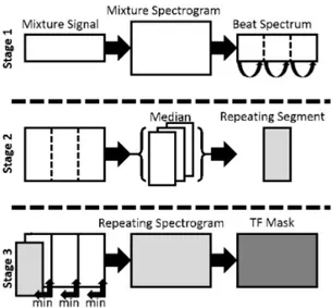
Figure 1.4 REPET: Building the repeating background model.In stage 1, we analyze the
mixture spectrogram and identify the repeating period. In stage 2, we split the mixture into patches of the identified length and take the median of them. This allows to extract their common part and hence the repeating pattern. In stage 3, we use this repeating pattern in each segment to construct a mask for separation.
straightforwardly provides an estimate of the PSD vj(n, f )of the two sources to use
for source separation as in chapter ??. The originality of the approach is that no ex-plicit parametric model was picked such as in NMF: each PSD was only defined as locally constant on some vertical or horizontal neighborhood depicted in figure 1.5 as kernels (a) and (b).
Whatever the harmonic complexity of the musical piece, this method achieves ex-cellent performance provided the harmonic sounds remain constant for a few frames, typically 200ms. The model is indeed not on the actual position of the partials, but rather on their duration and steadiness. This proves extremely robust in practice when only separating drum sounds is required.
1.4.2
REPET: separating repeating background
HPSS exploits local regularity in the most straightforward way: the PSD of a source is assumed constant in neighboring TF bins, either horizontally or vertically. However, a natural extension would be to consider longer term dependencies. In this respect, an observation made in (Rafii and Pardo, 2011) is that the musical accompaniment of a song often has a spectrogram that is periodic. In other words, whatever the particular drum loop or guitar riff to be separated from vocals, it often comes as repeated over and over again in the song, while the vocals are usually not very repetitive.
Taking the repeating nature of musical accompaniment into account in a non-parametric way leads to the REPET algorithm presented originally in (Rafii and Pardo, 2011, 2013) and summarized in figure 1.4. Its first step is to identify the period at which the PSD of the accompaniment is repeating. In practice, this is done by picking the most predominant peaks of a tempo detection feature such as the beat spectrogram. Then, the PSD of the accompaniment is estimated as a robust averaging of its different repetitions. Time-domain signals are produced by a classical spectral subtraction method, as presented in chapter ??.
The most interesting feature of REPET is that it allows capturing a wide variety of musical signals using only a single parameter, which is the period of the accompa-niment. Most other separation models (e.g. NMF) require estimating a much larger number of parameters and have many more meta parameters to adjust (e.g. number of basis functions, loss function, method of seeding the activation matrix, etc.) In its original form, REPET assumes a strictly repetitive accompaniment, which is not realistic for full-length tracks except for some electronic songs. It was extended to slowly varying accompaniment patterns in (Liutkus et al., 2012), yielding the adap-tive aREPET algorithm.
1.4.3
REPET-sim: exploiting self-similarity
REPET and aREPET are approaches to model the musical accompaniment with the only assumption that its PSD will be locally periodic. From a more general per-spective, this may be seen as assuming the each part of the accompaniment can be found elsewhere in the song, only superimposed with incoherent parts of the vocals. The specificity of REPET in this context is to provide a way to identify these similar parts as juxtaposed one after the other. In some cases like a rapidly varying tempo or such complex rhythmic structures, this simple strategy may be inappropriate. In-stead, when attempting to estimate the accompaniment at each time frame, it may be necessary to adaptively look for the similar parts of the song, no longer assumed as located fixed periods away.
The idea behind the REPET-sim method (Fitzgerald, 2012) is to exploit this
self-similarityof the accompaniment. It works by first constructing a N × N similarity
matrix that indicates which frames are close to one another under some spectral sim-ilarity criterion. Then, the PSD of the accompaniment is estimated for each frame as a robust average of all frames in the song that were identified as similar. REPET and aREPET appear as special cases of this strategy when the neighbors are constrained to be regularly located over time.
In practice, REPET-sim leads to good separation performance, as long as the sim-ilarity matrix for the accompaniment is correctly estimated. The way simsim-ilarity be-tween two frames is computed hence appears as a critical choice for it to work. While more sophisticated methods may be proposed in the future, simple correlations be-tween each frame of the mixture spectrogram |X| was already shown as giving good results in practice. In any case, REPET-sim is a method bridging music information retrieval with audio source separation.
Figure 1.5 Examples of kernels to use in Kernel Additive Model (KAM) for modeling
(b) percussive, (b) harmonic, (c) repetitive and (d) spectrally smooth sounds
1.4.4
KAM: Nonparametric modeling for spectrograms
The REPET algorithm and its variants focus on a model for only one of the signals to separate: the accompaniment. They can be understood as ways to estimate the PSD of this one source given the mixture spectrogram |X|. Then, separation is performed by spectral subtraction or some variant, producing only two separated signals. Similarly, HPSS may only be used to separate harmonic and percussive components.
To improve the performance of REPET, it was proposed in (Rafii et al., 2013, 2014) to combine it with a parametric spectrogram model based on NMF for the vocals. In practice, a first NMF decomposition of the mixture is performed that produces a PSD model for both vocals and accompaniment. Then, this preliminary accompaniment model is further processed using REPET to enforce local repetition. A clear advantage of this approach is that it doesn’t leave the vocal model totally unconstrained as in REPET alone, which often leads in increased performance. In the same vein, the methodology proposed in (Tachibana et al., 2014; Driedger and Müller, 2015) sequentially applies HPSS with varying length-scales in a cascade fashion. This allows the separation not only of harmonic and percussive parts using HPSS, but also vocals and residual.
A general framework to gather both HPSS and REPET under the same umbrella and to allow for arbitrary combinations between them and also other PSD models was introduced in (Liutkus et al., 2014) and named Kernel Additive Modeling (KAM). It was then instantiated for effective music separation in (Liutkus et al., 2015). In essence, the basic building blocks of KAM for music separation are the same as the Gaussian probabilistic model presented in chapter ??. The only fundamental difference lies in the way the PSD vj(n, f )of the sources are modeled and estimated.
The specificity of KAM for spectral modeling is to avoid picking one single and global parametric model to describe vj(n, f )as in the various approaches such as
NMF described in chapter ??. Instead, the PSD vj(n, f )of each source j at TF bin
(n, f )is simply assumed constant on some neighborhood Ij(n, f ):
∀ (n0, f0) ∈ Ij(n, f ) , vj(n0, f0) ≈ vj(n, f ) . (1.2)
For each TF bin (n, f), the neighborhood Ij(n, f )is thus the set of all the TF
bins for which the PSD should have a value close to that found at (n, f). This kind of model is typical of a nonparametric kernel method: it does not impose a global
fixed form to the PSD, but just constrain it just locally. Several examples of such kernels are given in figure 1.5, that correspond to the different methods discussed in the previous sections. REPETsim can easily be framed in this context by introducing the similarity matrix and thresholding it to construct Ij.
As can be seen, KAM generalizes the REPET and HPSS methods by enabling their combination in a principled framework. Each source is modeled using its own kernel, or alternatively using a more classical parametric model such as a NMF. Then, the iterative estimation procedure is identical as in the Expectation-Maximization (EM) method presented in chapter ??, except for the Maximization step that needs to be adapted for sources modeled with a kernel. Indeed, lacking a unique global parametric model, the concept of maximum likelihood estimation of the parameters does not make sense anymore. Hence, an approach is to replace it by a model cost
functionthat accounts for the discrepancies between the PSD estimate and its values
at neighboring values. In (Liutkus et al., 2015), the absolute error was picked: vj(f, n) ←argmin v X (f0,n0)∈I j(f,n) |v −pbj(n 0, f0)| , (1.3)
wherepbj(n, f )was defined in chapter ?? and corresponds to the unconstrained esti-mate of the PSD of source j obtained during the preceding E-step of the algorithm. It is straightforward that this choice amounts to simply process zjwith a median filter
to estimate vj: equation 1.3 is equivalent to:
vj(f, n) ←median {zj(n0, f0) | (n0, f0) ∈ Ij(n, f )} . (1.4)
In the case the neighborhoods Ij are shift-invariant, operation 1.4 can be
imple-mented efficiently as a running median filter with linear complexity, yielding a com-putationally cheap parameter estimation method.
The KAM framework provides a common umbrella for methods exploiting local regularities in music source separation, as well as for their combination with paramet-ric models. It furthermore allows their straightforward extension to the multichannel case, benefiting from the Gaussian framework presented in depth in chapter ??.
1.5
Taking advantage of multiple instances
The previous section focused on exploiting redundancies within the same song to perform source separation. Doing so, the rhythmic structure inherent to music signals can be leveraged to yield efficient algorithms for fast source separation.
In this section, we show how some application scenarios in music signal processing come with further redundancies that may exploited to improve separation. In some cases indeed, apart from the mixture to separate, other signals are available that fea-ture some of the sources to separate, possibly distorted and superimposed with other interfering signals. In general, this scenario can be referred to as source separation using deformed references (Souviraa-Labastie et al., 2015a).
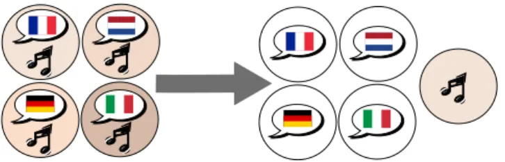
Figure 1.6 Using the audio tracks of multiple related videos to perform source separation.
Each circle on the left represents a mixture containing music and vocals in the language associated with the flag. The music is the same in all mixtures. Only the language varies. Given multiple copies of a mixture where one element is fixed lets one separate out this stable element (the music) from the varied elements (the speech in various languages).
1.5.1
Common signal separation
Back-catalog exploitation and remastering of legacy movie content may come with specific difficulties concerning the audio soundtrack. For very old movies, adverse circumstances such as fires in archive buildings may have lead the original music and dialogue separated soundtracks to be lost. In this case, all that is available are the stereophonic or monophonic downmixes. However, making a restored version of the movie at professional quality comes with the requirement of not only remastering its audio content, but also upmixing it (taking one or two tracks and turning it into many more tracks) to modern standards such as 5.1 surround sound. In such a situation, it is desirable to recover estimates of the music and dialogue soundtracks using source separation techniques.
Even if the original tracks may be lost, a particular feature of movie soundtracks is that they most often come in several languages. These many versions are most likely to feature the same musical content, superimposed with a language-specific dialogue track. The situation is depicted in figure 1.6. The objective of common signal sepa-ration in this context becomes to recover the separated dialogues and common music tracks based on the international versions of the movie. An additional difficulty of this scenario is that the music soundtrack is not identical in all international versions. On the contrary, experience shows that mixing and mastering was usually performed independently for all of them. We generally arbitrarily pick one of the international version as the one we wish to separate, taking others as deformed references.
A method for common signal separation was presented in (Leveau et al., 2011). It is a straightforward application of the coupled NMF methodology thoroughly pre-sented in chapter ??. Let us consider for now the case of I very old monophonic in-ternational versions of the same movie, denoted xi, with Short Term Fourier
Trans-form xi(n, f ). We assume all versions have the same length. The model picked
in (Leveau et al., 2011) decomposes each version xias the sum of a common
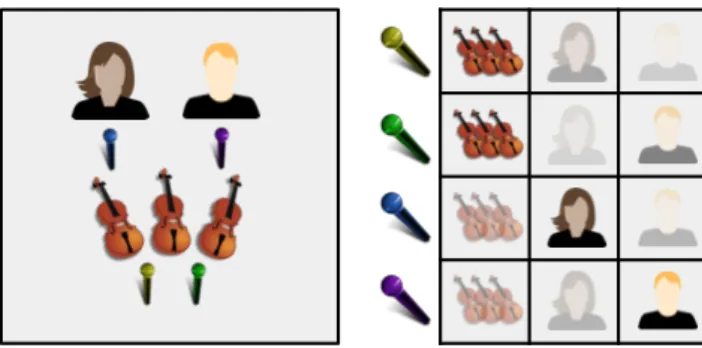
Figure 1.7 Interferences of different sources in real-world multitrack recordings. Left:
microphone setup. Right: interference pattern (courtesy of R. Bittner and T. Prätzlich)
each cij as in chapter ??:
cij(n, f ) ∼ Nc(0, vij(n, f )) . (1.5)
The method then assigns a standard NMF model for the version-specific PSD Vi2=
BiHi, and constrains the common signals ci1(n, f )to share the NMF model, up to
a version-specific filter: Vi1= Diag (gi) BcHc, where giis a nonnegative F × 1
vector modeling the deformation applied on reference i. As usual, all B and H matrices gather NMF parameters and are of a user-specified dimension.
Putting this all together, the ithinternational version x
i(n, f )is modeled as
Gaus-sian with variance Vitaken as:
Vi= BiHi
| {z } dialogues fori
+ Diag (gi) BcHc
| {z }
filtered common part
. (1.6)
Given the model 1.6, inference of the parameters using the standard methodology presented in chapter ?? is straightforward. Once the parameters have been estimated, the separated components can be separated through Wiener filtering.
1.5.2
Multi-reference bleeding separation
Studio recordings often consist in different musicians all playing together, with a set of microphones capturing the scene. In a typical setup, each musician or orchestral instrumental group will be recorded by at least one dedicated microphone. Although a good sound engineer does his best to acoustically shield each microphone from sources other than its target, interferences are inevitable and often denoted bleeding in the sound engineering parlance. The situation is depicted on figure 1.7, whose left part shows an exemplary recording setup, while the right part illustrates the fact that each recording will feature interferences from all sources in varying proportions.
Dealing with multitrack recordings featuring some amount of bleeding has always been one of the daily duty of professional sound engineers. In the recent years, some
research was conducted to design engineering tools aimed at reducing those interfer-ences (Kokkinis et al., 2012; Prätzlich et al., 2015). In the remainder of this section, we briefly present the Multitrack Interference RemovAl (MIRA) model presented in (Prätzlich et al., 2015).
As usual, let J be the number of sources — the different musicians — and let xi
be the single channel signal captured by microphone i. The MIRA model comes with two main assumptions. First, all the recordings xi are assumed independent.
This amounts to totally discard any phase dependency that could be present in the recordings and proved a safe choice in case of very complex situations such as the real-world orchestral recordings considered in (Prätzlich et al., 2015). Second, each recording is modelled using the Gaussian model presented in chapter ??:
xi(n, f ) ∼ Nc(0, vi(n, f )) , (1.7)
where vi is the PSD of recording i. Then, this PSD is decomposed as a sum of
contributions originating from all the J sources in the following way: vi(n, f ) =
J
X
j=1
λijvj(n, f ) , (1.8)
where vj stands for the PSD of the latent source j and the entry λij ≥ 0of the
interference matrixindicates the amount of bleeding of source j in recording i. If
desired, the source PSD vjcan be further constrained using either a NMF or a kernel
model as presented above.
Although it is very simple and discards phase dependencies, this model has the nice feature of providing parameters that are readily interpretable by sound engi-neers. Given a diagram of the acoustic setup, it is indeed straightforward for a user to initialize the interference matrix. Then, the MIRA algorithm iterates estimation of vjand λij. A critical point for this algorithm to work is that we know that each
source is predominant in only a few recordings. Only those are hence used to es-timate vj. Then, given the sources PSD vj, the interference matrix can readily be
estimated using classical multiplicative updates as presented in chapter ??.
Once the parameters have been estimated, separation can be achieved by estimating the contribution cij of source j in any desired recording xiusing classical Wiener
filter: b cij(n, f ) = λijvj(n, f ) P j0λij0vj0(n, f ) xi(n, f ) . (1.9)
MIRA was shown to be very effective for interference reduction in real orchestral recordings featuring more than 20 microphones and sources (Prätzlich et al., 2015). 1.5.3
A general framework: reference-based separation
As can be noticed, the methods described in the preceding sections may all be gath-ered under the same general methodology, that puts together the recent advances
made in NMF and in probabilistic modeling for audio, see chapters ?? and ??, re-spectively.
In this common framework for separation using multiple deformed references pre-sented in (Souviraa-Labastie et al., 2015a), the signals analyzed are not only those to be separated, but also auxiliary observations that share some information with the sources to recover. The main idea of the approach is parameter sharing among observations.
In short, the SPORES framework (SPOtted Reference-based Separation) models all observations using a NMF model where some parameters may be assumed com-mon to several signals, but deformed from one to another by the introduction of time and frequency deformation matrices. The whole approach is furthermore readily extended to multichannel observations.
Apart from the applications briefly mentioned above, it is noticeable that the same kind of framework may be applied in other application settings, such as text-informed music separation (Magoarou et al., 2014) or separation of songs guided by cov-ers (Souviraa-Labastie et al., 2015b).
In all these cases, a very noticeable feature of the approach is that it fully exploits music-specific knowledge for assessing which parameters of the target mixture may benefit from the observation of the reference signals. For instance, while the pitch information of a spoken reference may be useless to model a sung target, its acoustic envelope can prove valuable for this purpose. In the case of covers, this same pitch information may be useful, although the particular timbre of the sources may change completely from one version to another.
1.6
Interactive Source Separation
Commonly-used algorithms for source separation, such as NMF, REPET and Si-nusoidal Modeling, are not designed to let the user specify which source from the mixture is of interest. As a result, even a successful separation may be a failure from the user’s perspective, if the algorithm separates the wrong thing from the mixture (you gave me the voice, but I wanted the percussion). Researchers working on audio source separation in a musical context have been at the forefront of making interactive systems that let the user guide separation in an interactive way.
Smaragdis and Mysore (2009) presented a novel approach to guiding source sepa-ration. The user is asked to provide a sound that mimics the desired source. For exam-ple, to separate a saxophone solo from a jazz recording, the user plays the recording over headphones and sings or hums along with the saxophone. This information is used to guide Probabilistic Latent Component Analysis (PLCA) (Smaragdis et al., 2006), a probabilistic framing of Non-negative Matrix Factorization.
The user records a sound that mimics the target sound (in frequency and temporal behavior) to be extracted from the mixture. The system estimates an M-component PLCA model from the user imitation. Then, the system learns a new N+M element PLCA model for the mixture to be separated. Here, N components are learned from
scratch, while the M components start with the values learned from the user record-ing. Once the system converges, the target of interest can be separated by using only the M elements seeded by the user vocalizations to reconstruct the signal.
Since not all sources are easily imitated by vocalization, Nick Bryan et al followed up this work by building a visual editor for NMF/PLCA source separation called the Interactive Source Separation Editor (ISSE) (Bryan et al., 2014). This editor displays the audio as a time-frequency visualization of the sound (e.g. a magnitude spectrogram). The user is given drawing and selection tools so they can roughly paint on time-frequency visualizations of sound, to select the portions of the audio for which dictionary elements will be learned and marked as the source of interest. They conducted users studies on both inexperienced and expert users and found that both groups can achieve good quality separation with this tool.
Zafar Rafii et al (Rafii et al., 2015) followed this work with an interactive source separation editor for the REPET algorithm. In this work, an audio recording is dis-played as a time-frequency visualization (a log-frequency spectrogram). The user then selects a rectangular region containing the element to be removed. The selected region is the n cross-correlated with the remainder of the spectrogram, to find other instances of the same pattern. The identified regions are averaged together to gener-ate a canonical repeating pattern. This canonical pattern is used as a mask to remove the repeating elements.
1.7
Crowd-based evaluation
The performance of today’s source separation algorithms are typically measured in terms of intelligibility of the output (in the case of speech separation), or with the commonly-used measures in the BSS-EVAL toolkit (Févotte et al., 2005) (Source to Distortion Ratio, Source to Interference Ratio and Source to Artifact Ratio). Several international campaigns regularly assess the performance of different algorithms, and the interested reader is referred to SiSEC (Ono et al., 2015) and MIREX2)for more pointers.
More recently, automated approaches to estimating the perceptual quality of sig-nals have been applied, the most prominent being PEASS (Vincent, 2012). As dis-cussed at the start of this chapter, commonly used measures for source separation quality may not always be appropriate in a musical context, since the goal of the separation may vary, depending on the application. An obvious alternative to using automated evaluation metrics with fixed definitions of "good" is to use humans as the evaluators. This lets the researcher define "good" in a task-dependent way.
The gold-standard evaluation measure for audio is a lab-based listening test, such as the MUSHRA protocol (ITU, 2014). Subjective human ratings collected in the lab are expensive, slow, and require significant effort to recruit subjects and run evalua-tions. Moving listening tests from the lab to the micro-task labor market of Amazon
Mechanical Turk can greatly speed the process and reduce effort on the part of the researcher.
Cartwright et al. (2016) compared MUSHRA performed by expert listeners in a laboratory to a MUSHRA test performed over the web, on a population of 530 par-ticipants drawn from Amazon Mechanical Turk. The resulting perceptual evaluation scores were highly correlated to those estimated in the controlled lab environment.
1.8
Some examples of applications
1.8.1
The good vibrations problem
The majority of the Beach Boys material recorded and released between 1965 and 1967 was long available in mono only. Some of the band’s most popular songs were released in that period and are included in albums as famous as Pet Sounds or Wild
Honey. As explained in (FitzGerald, 2013), the choice of the monophonic format
first comes out of a preference of the band’s main songwriter and producer Brian Wilson, and then is also due to the way some tracks were recorded and produced. As extraordinary as it may seem today, overdubs were in some cases directly recorded live during mixdown. Of course, this gives a flavor of uniqueness and spontaneity to the whole recording process, but also means that simply no version of the isolated stems would ever be available, at least not until 2012.
In 2012, the Beach Boys’ label was willing to release stereo versions of those tracks for the first time. Some of the tracks for which the multitrack session was available had already been released in stereo during the 90s. However, for some tracks as famous as Good Vibrations, only the monophonic downmix was available. Hence, Capitol records decided to contact researchers in audio signal processing to see if something could be done to get back the stems from the downmix, permitting stereo remastering of the songs. Music source separation appeared as the obvious way to go.
As mentioned in (FitzGerald, 2013) that reports the event, the various techniques used for upmixing those legacy songs include various combinations of the methods we discussed in this chapter. For instance, both the accompaniment alone and the downmix were available in some cases, but not isolated stems such as vocals that were overdubbed during mixdown. In that case, common signal separation as dis-cussed above in section 1.5.1 could be applied to recover the isolated lost stems. In other cases, only the downmix was available and blind separation was the only op-tion to recover separated signals. Depending on the track, various techniques were considered. To separate drums signals, HPSS as described in section 1.4.1 was used. For vocals, FitzGerald (2013) reports good performance of the REPET-sim method presented in section 1.4.3. Then, instrument-specific models such as the variants of NMF presented in section 1.2.2 were involved to recover further decomposition of the accompaniment track.
Of course, the separated tracks that were obtained using all those techniques are in no way as clean as original isolated stems could have been. However, they were good enough for the sound engineers involved in the project to produce very good stereophonic upmixed versions of tracks that had never been available in a format different than mono. These remastered versions were released in 2012.
1.8.2
Reducing drum leakage: Drumatom
As mentioned in section 1.5.2, multitrack recording sessions often feature leakage of the different sounds into all microphones, even in case of professional quality record-ings. This problem is particularly noticeable for of drum signals, that routinely end up as perfectly audible in most of the simultaneous recordings of the session. This is due to the very large bandwidth of those signals. Such leakage is an important issue that sound engineers have to face, because it raises many difficulties when mixing the tracks or when slightly modifying the time alignment of the stems.
The MIRA algorithm briefly summarized in section 1.5.2 builds on previous re-search on interference reduction that is described, e.g. in (Kokkinis et al., 2012). The fact is that this previous research actually developed out of academia into a very successful commercial audio engineering tool called Drumatom, produced by the Accusonus company3). Drumatom notably includes many enhancements of the algorithm specialized for percussive signals, as well as real time implementation and good-looking professional graphical user interface. The whole project is presented in (Kokkinis et al., 2013).
As highlighted in (Kokkinis et al., 2013) but also in (Vaneph et al., 2016), the objective of devising professional audio engineering software based on source sep-aration is not to create completely automated tools. Indeed, experience shows that source separation methods in the case of music systematically feature some kind of trade-off between separation and distortion. In essence, it is possible to process the recordings so that interference are not audible, but this may come at the price of too large a distortion, leading to perceptually poor results. For this reason and depend-ing on the application, the tundepend-ing of parameters must be performed by an end-user. In the case of leakage reduction, these facts are shortly discussed in the perceptual evaluation presented in (Prätzlich et al., 2015).
It is hence clear that apart from research conducted in music signal processing, an important research and development effort is also required in the field of human-computer interaction to create tools that end up as actually being useful to practition-ers.
1.8.3
Impossible duets made real
Since music is a powerful means for artistic creativity, managing the demixing of mu-sical content through source separation necessarily has deep artistic consequences. Indeed, the impact of source separation is not limited to upmixing and remastering songs to reach unprecedented levels of quality. It also makes it possible to use sep-arated signals from existing tracks as raw material for artistic creativity, yielding a whole new range of possibilities.
In the electronic music scene, including existing recordings into new tracks has long been known and acknowledged under the name of sampling and this practice is now widely spread across all of musical genres. Still, sampling has always been lim-ited either to excerpts of downmixes, or to already available isolated sounds. Source separation makes it possible for an artist to reuse drumloops or vocals from within another song to create new original creations.
This scenario is presented in (Vaneph et al., 2016) as a groundbreaking opportunity for artists to create exciting new music. In particular, "impossible duets" between two artists that never met in real life are made possible by separating vocals and embedding them into new recordings.
Of course, going from the laboratory to actual artistic creation and to methods that may be used in practice by musicians is far from trivial. Apart from the already mentioned important effort required in the design of graphical user interfaces, the separated results often greatly benefit from post-processing using dedicated audio engineering techniques. This is for instance what motivates Audionamix4)to have sound engineers working in close collaboration with researchers in signal process-ing for the design of their separation softwares. The interested reader is referred to Vaneph et al. (2016) for more details.
1.9 Summary
In this chapter, we have covered a broad range of source separation algorithms applied to music and, often, to audio tracks of videos. While we have attempted to also provide broad coverage in our referencing of work applied to music, space prohibits describing every method in detail. Where appropriate, we reference other chapters to provide algorithmic detail of approaches that are used across many types of audio. We have also attempted to include sufficient detail on representative music-specific algorithms and approaches not covered in other chapters. The intent is to give the reader a high-level understanding of the workings of key exemplars of the source separation approaches applied in this domain. We strongly encourage the reader to explore the works cited in the bibliography for further details.