HAL Id: hal-00164877
https://hal.archives-ouvertes.fr/hal-00164877
Submitted on 24 Jul 2007
HAL is a multi-disciplinary open access
archive for the deposit and dissemination of sci-entific research documents, whether they are pub-lished or not. The documents may come from teaching and research institutions in France or abroad, or from public or private research centers.
L’archive ouverte pluridisciplinaire HAL, est destinée au dépôt et à la diffusion de documents scientifiques de niveau recherche, publiés ou non, émanant des établissements d’enseignement et de recherche français ou étrangers, des laboratoires publics ou privés.
Daniel Kanaan, Philippe Wenger, Damien Chablat
To cite this version:
Daniel Kanaan, Philippe Wenger, Damien Chablat. Workspace and Kinematic Analysis of the VERNE machine. AIM, Sep 2007, Zürich, Switzerland. pp.1-6. �hal-00164877�
Abstract— This paper describes the workspace and the
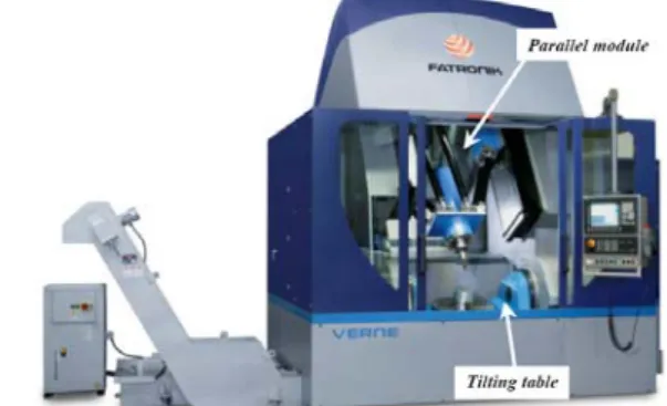
inverse and direct kinematic analysis of the VERNE machine, a serial/parallel 5-axis machine tool designed by Fatronik for IRCCyN. This machine is composed of a three-degree-of-freedom (DOF) parallel module and a two-DOF serial tilting table. The parallel module consists of a moving platform that is connected to a fixed base by three non-identical legs. This feature involves (i) a simultaneous combination of rotation and translation for the moving platform, which is balanced by the tilting table and (ii) workspace whose shape and volume vary as a function of the tool length. This paper summarizes results obtained in the context of the European projects NEXT (“Next Generation of Productions Systems”).
I. INTRODUCTION
ARALLEL kinematic machines (PKM’s) are well known for their high structural rigidity, better payload-to-weight ratio, high dynamic performances and high accuracy [1-3]. Thus, they are prudently considered as attractive alternatives designs for demanding tasks such as high-speed machining [4].
A well-known feature of PKM is the existence of multiple solutions to the direct kinematic problem. That is, the moving platform can admit several positions and orientations (poses) in the workspace for one given set of input joint values [5]. Moreover, parallel manipulators exist with multiple inverse kinematic solutions. This means that the moving platform can admit several input joint values corresponding to one given pose of the end-effector [6]. For industrial PKMs, the resolution of the direct and inverse kinematic problems is usually made using iterative methods. With such methods, the calculation time can change as function of the configuration of the PKM. A major drawback of PKMs is a complex workspace. The workspace of a PKM has not a simple geometric shape, and its functional volume is reduced as compared to the space occupied by the machine [7].
D. Kanaan is with the Institut de Recherche en Communications et Cybernétique de Nantes (IRCCyN) (UMR CNRS 6597), France (corresponding author to provide phone: 240376958; fax: 33-240376930, e-mail: [email protected]); P. Wenger is with the IRCCyN (UMR CNRS 6597), France (e-mail: [email protected]); D. Chablat is with the IRCCyN (UMR CNRS 6597), France (e-mail: [email protected]).
Because many industrial tasks require less than six degrees of freedom, several lower-DOF PKMs have been developed. For some of theme, the reduction of the number of DOFs can result in coupled motions of the moving platform [8-10]. This is the case, for example, in the RPS manipulator [9] and in the parallel module of the VERNE machine. The kinematic modeling of these PKMs must be done case by case according to their structure.
Many researchers have contributed to the study of the kinematics of lower-DOF PKMs. Many of them have focused on the discussion of both analytical and numerical methods [11-12]. This paper investigates the workspace and the inverse and direct kinematics analysis of the VERNE machine (Fig. 1).
Fig. 1. Overall view of the VERNE machine
The following section describes the VERNE machine. In section III, we study the kinematics of the VERNE machine. In section IV, we present the workspace calculation for different tool length and for different orientation angle of the tool. Finally Section V concludes this paper.
II. DESCRIPTION OF THE VERNE MACHINE
The VERNE machine consists of a parallel module and a tilting table as shown in Fig. 2. The vertices of the moving platform of the parallel module are connected to a fixed-base plate through three legs Ι, ΙΙ and ΙΙΙ. Each leg uses a pair of rods linking a prismatic joint to the moving platform through two pairs of spherical joints. Legs ΙΙ and ΙΙΙ are two identical parallelograms. Leg Ι differs from the other two legs in that A A11 12≠B B11 12, where A (respectively ij
Workspace and Kinematic Analysis of the VERNE machine
Daniel KANAAN, Philippe WENGER and Damien CHABLAT
ij
B ) is the center of spherical joint number j on the
prismatic joint number i (respectively on the moving platform side), i = 1..3, j = 1..2. The movement of the moving platform is generated by three sliding actuators along three vertical guideways.
ΙΙ Ι ΙΙΙ x y z xp yp z p xt zt yt da dt Tilting axis Δ U
Fig. 2: Schematic representation of the VERNE machine
Due to the arrangement of the links and joints, legs ΙΙ and ΙΙΙ prevent the platform from rotating about y and z axes. Leg Ι prevents the platform from rotating about z-axis (Fig. 2) because A A11 12≠B B11 12, however, a slight coupled
rotation α about x-axis exists. The tilting table is used to rotate the workpiece about two orthogonal axes. The first one, the tilting axis, is horizontal and the second one, the rotary axis, is always perpendicular to the tilting table. This machine takes full advantage of these two additional axes to adjust the tool orientation with respect to the workpiece.
III. KINEMATIC ANALYSIS OF THE VERNE MACHINE
A. Kinematic equations of the VERNE machine
In order to analyze the kinematics of the VERNE machine, three relative coordinates are assigned as shown in Fig. 2. A static Cartesian frame Rb =( , , , )O x y z is fixed at the base of the machine tool, with the z-axis pointing downward along the vertical direction. Two mobile Cartesian frame, the first frame Rpl =( ,P xP, , )yP zP , is
attached to the moving platform at point P and the second frame, R t xt( , , , )t yt z is attached to the tilting table at t
point t. Let us b pl
T define the transformation matrix that
brings the fixed Cartesian frame R on the frame b R pl
linked to the moving platform.
(
, ,)
(
,)
b
pl p p p
T =Trans x y z Rot x α (1)
We use this transformation matrix to express B as ij
function of xp, , yp zp and α by using the relation
b pl ij pl ij
B = T B where pl ij
B represents the point B ij
expressed in the frame Rpl.
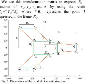
-600 -400 -200 0 200 400 600 -800 -600 -400 -200 0 200 400 600 800 P A11 B11 A12 B12 A21 B21 A22 B22 A31 B31 A32 B32 r4 y x yP xP R2 d2 D2 R1 D1 r1 d1 2r3 2r2
Fig. 3: Dimensions of the parallel kinematic structure
Using the parameters defined in Figs. 2 and 3, the constraint equations of the parallel manipulator are expressed as:
(
) (
)
(
)
(
)
2 2 2 2 0 1..3, 1..2Bij Aij Bij Aij Bij Aij i
x x y y
z z L i j
− + − +
− − = = = (2)
Leg Ι is represented by two different Eqs. (3-4). This is due to the fact that A A11 12≠B B11 12 (figure 3).
(
) (
)
(
)
2 2 1 1 1 1 2 2 1 1 1 cos( ) sin( ) 0 P P P x D d y R r z R L α α ρ + − + + − + + − − = (3)(
) (
)
(
)
2 2 1 1 1 1 2 2 1 1 1 cos( ) sin( ) 0 P P P x D d y R r z R L α α ρ + − + − + + − − − = (4)Leg ΙΙ is represented by a single Eq. (5).
(
) (
)
(
)
2 2 2 2 2 4 2 2 2 2 2 cos( ) sin( ) - 0 P P P x D d y R r z R L α α ρ + − + − + + − − = (5)The leg ІІІ, which is similar to leg ІІ (figure 3), is also represented by a single Eq. (6).
(
) (
)
(
)
2 2 2 2 2 4 2 2 2 3 3 cos( ) sin( ) 0 P P P x D d y R r z R L α α ρ + − + + − + + − − = (6) θ1 φ2 θ2 φ1 Tilting axis ToolFig. 4: Draw of the tilting table where the tool orientation is defined by (φ1, φ2) relative to Rt and the orientation of the tilting table is defined by
Let b t
T define the transformation matrix that brings the
fixed Cartesian frame Rb on the frame Rt linked to the
tilting table.
1 2
( , ) ( , ) ( , ) ( , ) ( , )
b
t a t
T =trans z d rot xθ trans z d rot xπ rot zθ (7)
Let t pl
T define the transformation matrix that brings the
frame Rt linked to the tilting table on the frame Rpl linked
to the moving platform; where Xu, Yu and Zu are the
coordinates of the tool centre point (TCP), U, in Rt.
2 1
( , , ) ( , ) ( , ) ( , )
t
pl u u u
T =trans X Y Z rot zφ rot xπ φ+ trans z −Δ
(8) We use transformation matrices from Eqs. (7) and (8) in
order to express B as function of ij Xu, Yu, Zu, φ 1, φ 2, 1
θ and θ by using the relation 2 b pl ij pl ij B = T B where b b t pl t pl T = T T and pl ij
B represents the point Bij expressed
in the frame R . pl
Using Eq. (2) and the parameters defined in Figs. 2, 3 and 4, we can express all constraint equations of the VERNE machine. However knowing that A Bi1 i1 and
2 2
i i
A B are parallel for i=1..2, we can prove that:
2 2
θ = −φ (9)
Substituting the above value of θ in all constraint 2
equations resulting from Eq. (1), we obtain that leg Ι is represented by two different equations (10) and (11) while leg ΙΙ (respectively leg ΙΙΙ) is represented by only one equation (12) (respectively equation 13)).
Equations (10-13) are not reported here because of space limitation. They are available in [14].)
If we identify Eqs. (10), (11), (12) and (13) with Eqs. (3), (4), (5) and (6) respectively, we conclude that:
1 1
α θ φ= + (14)
The constraint equations of the VERNE machine will be used in order to obtain the inverse kinematic models of the full VERNE machine.
B. Coupling between the position and the orientation of the platform
The parallel module of the VERNE machine possesses three actuators and three degrees of freedom. However, there is a coupling between the position and the orientation angle of the platform. The object of this subsection is to study the coupling constraint imposed by leg I.
By eliminating ρ from Eqs. (3) and (4), we obtain a 1
relation (15) between xP, yP and α independently of zP.
(
)
(
)
(
)
(
)
2 2 2 2 2 2 1 1 1 1 1 1 1 2 2 2 2 2 1 1 1 1 1 1 sin ( ) 2 cos( ) sin ( ) 2 cos( ) 0 P P R x D d r R r R y R L R r R r α α α α + − + − + − − + − = (15)We notice that for a given α , Eq. (15) represents an ellipse (16). The size of this ellipse is determined by a and
b , where a is the length of the semi major axis and b is
the length of the semi minor axis.
(
)
2 2 1 1 2 2 1 P P x D d y a b + − + = (16) where(
)
(
)
(
)
(
)
(
)
2 2 2 1 1 1 1 1 2 2 2 2 2 1 1 1 1 1 1 2 2 1 1 1 1 2 cos( ) sin ( ) 2 cos( ) 2 cos( ) a L R r R r R L R r R r b r R r R α α α α ⎧ = − + − ⎪ ⎪ ⎨ − + − ⎪ = ⎪ − + ⎩These ellipses define the locus of points reachable with the same orientation α .
C. The Inverse Kinematics
For the inverse kinematic problem of the parallel module, the position coordinates (xP, , yP z ) are given but P
the coordinates ρi (i=1..3) of the actuated prismatic joints and the orientation angle α of the moving platform are unknown. The problem consists in solving the system ( 1)S
of 4 equations (3-6) for only 4 unknowns (ρi (i=1..3) and α ). Thus, the position of the TCP (Xu, , Yu Z ) and the u
orientation of the tool (φ1 and φ ) are given relative to the 2
frame R , but the joint coordinates, defined by the position t
( 1..3)
i i
ρ = of the actuated prismatic and the orientation (θ1 and θ ) of the tilting table in the base frame 2 R are b
unknown. Knowing that θ2 = − from Eq. (9), the φ2 problem consists in solving the system ( 2)S of 4
equations ((10), (11), (12) and (13)) for only 4 unknowns (ρi (i=1..3) and θ ). 1
In both cases, we follow the same reasoning to solve the inverse kinematics. Due to space limitation, we present only the inverse kinematic model of the full VERNE machine. The inverse kinematic model of the parallel module can be obtained easily by considering system ( 1)S
instead of system ( 2)S (see [13]).
First, we eliminate ρ from Eqs. (10) and (11) in order 1 to obtain a relation (17) between the TCP position and orientation (Xu, ,Y u Zu, φ , 1 φ ) and the tilting angle 2 θ . 1
Then, we find all possible orientation angles θ for 1
prescribed values of the position and the orientation of the tool. These orientations are determined by solving a six-degree-characteristic polynomial in tan( / 2)θ1 derived
from Eq. (17). This polynomial can have up to four real solutions. This conclusion is verified by the fact that
1 1
θ = − from Eq. 30 where α can have only four real φ α solutions (which can be proved by drawing together all ellipses of iso-values of α , see [13]). After finding all the possible orientations, we use the system of equations ( 2)S
to calculate the joint coordinates ρ for each orientation i angle θ . 1
For ρ we must verify that the values of 1, ρ obtained 1 from Eqs. (10) and (11) are the same. As a result, we eliminate one of the two solutions.
Observing the above remark and knowing from [16] that Eqs (10-11), (12), (13) are defined as two-degree-polynomials in , 1..3ρi i= respectively, we conclude that
there are four solutions for leg Ι and two solutions for leg ΙΙ and ΙΙΙ. Thus there are sixteen inverse kinematic solutions for the VERNE machine.
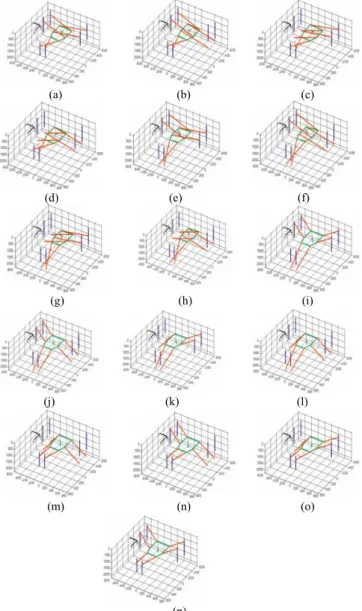
From the sixteen theoretical inverse kinematics solutions shown in Fig. 5, only one is used by the VERNE machine: the one referred to as (p) in Fig. 5, which is characterized by the fact that each leg must have its slider attachment points above the moving platform attachment points.
(a) (b) (c) (d) (e) (f) (g) (h) (i) (j) (k) (l) (m) (n) (o) (p)
Fig 5: The sixteen solutions to the inverse kinematics problem when -240 mm,
P
x = yP=-86 mm and zP=1000 mm
For the remaining 15 solutions one of the sliders leaves its joint limits or the two rods of leg I cross. Most of these solutions are characterized by the fact that at least one of the legs has its slider attachment points lower than the moving platform attachment points. To prevent rod
crossing, we also add a condition on the orientation of the moving platform. This condition is R1cos(θ φ1+ 1)> . r1
Finally, we check the joint limits of the sliders and the serial singularities [10].
Applying the above conditions will always yield a unique solution for practical applications. The proposed method for calculating the various solutions of the inverse kinematic problem has been implemented in C++. We are working with AMTRI, a UK industry, on implementing this code in a simulation package of PKMs, Visual Components.
D. The Forward Kinematics
For the forward kinematics of our spatial parallel manipulator, the values of the joint coordinates
( 1..3)
i i
ρ = are known and the goal is to find the coordinates x , P y and P z of the centre of the moving P
platform P.
To solve the forward kinematics, we successively eliminate variables x , P y and P z from the system ( 1)P S
of four equations (3-6) to lead to an equation function of the joint coordinates ρi (i=1..3) and function of the orientation angle α of the platform. To do so, we first compute y as function of P z by subtracting equation (3) P
from equation (4) and we replace this variable in system ( 1)S to obtain a new system ( 3)S of three equations (18),
(19) and (20) derived from equations (3), (5) and (6) respectively. We then compute z as function of P
( 1..3)
i i
ρ = and α by subtracting equation (19) from equation (20). We replace this variable in system ( 3)S to
obtain a new system ( 4)S of two equations (21) and (22)
derived from equations (18) and (19) respectively. Finally, we compute x as function of P ρi (i=1..3) and α by
subtracting equation (21) from equation (22) and we replace this variable in the system ( 4)S in order to
eliminate x . Equations of system ( ) (i=3..4)P Si are not
reported here because of space limitation. They are available in [14].
For each step, we determine solutions existence conditions by studying the denominators that appear in the expressions of x , P y and P z . These conditions are: P
1cos( ) 1 0
R α − ≠ (23) r
(
ρ2−ρ3)(
R1cos( )α −r1)
+2sin( )α(
r R4 1−r R1 2)
≠0 (24)Equation (23) implies that A B1 1 is perpendicular to the
slider plane of leg І. In this case equation (16) represents a circle because a b= .
When ρ ρ in equation (24), we have 2= 3 α ={0, }π . This means that yP = (obtained from Equations. 0 (5)−(6)).
tangent-half-angle substitution s=tan( / 2)α . As a consequence, the forward kinematics of our parallel manipulator results in a eight-degree-characteristic polynomial in s , whose coefficients are relatively large expressions in ρ , 1 ρ and 2 ρ . 3
(a) (b)
(c) (d) Fig. 6: The four assembly-modes of the VERNE parallel module for
1 674 mm,
ρ = ρ =2 685 mm and ρ3=250 mm. only (a) is reachable by
the actual machine
For the forward kinematics of the VERNE machine, the values of the joint coordinates, defined by the position
( 1..3)
i i
ρ = of the actuated prismatic and the orientation (θ1 and θ ) of the tilting table in the base frame 2 R are b
known and the goal is to find the position of the TCP (Xu, , Yu Z ) and the orientation of the tool (u φ1 and φ ) in 2
the frame R . t
Knowing that φ2 = − and θ2 φ α θ1= − from Eqs (9) and 1 (14), we solve this problem by first solving the forward kinematics of the parallel module of the VERNE machine in order to find the coordinates x , P y and P z of the P
centre of the moving platform P and the orientation α of the moving platform in term of the joint coordinates
( 1..3)
i i
ρ = . We then use transformation matrices from Eqs. (1) and (7) in order to express the tool position and orientation (Xu, , , Yu Zu φ1 and φ ) as function of 2
(
xP,yP, , ,zP θ θ . 1 2)
1 t t b t b pl b b pl b b pl t pl U= T U = T T U = T− T U (25) where pl[
0 0 1]
T U = Δ and t[
1]
T u u u U= X Y Zrepresent the TCP, ,U expressed in frames R (linked to pl
the moving platform) and the base frame R respectively. b
Finally we obtain:
1 1 2 2 2 2
2 2 1
and sin( ) 1cos( )
cos( ) 1sin( ) sin( ) 2
u p u p u p Y x V X x V Z y V φ α θ φ θ θ θ θ θ θ = − = − = − + ⎧ ⎧ ⎨ = + ⎨ = + ⎩ ⎩ (26) where V1= sin(Δ α θ− 1) cos( )− θ1 yp−sin( )θ1
(
zp−da)
and1 1 1
2 t cos( ) p acos( ) cos( )
V =d − θ z +d θ − Δ α θ−
For the VERNE machine, only 4 assembly-modes have been found (figure 6). It was possible to find up to 6 assembly-modes but only for input joint values out of the reachable joint space of the machine. Only one assembly-mode is actually reachable by the machine (solution (a) shown in Fig. 6) because the other ones lead to either rod crossing, collisions, or joint limit violation. The right assembly mode can be recognized, like for the right working mode, by the fact that each leg must have its slider attachment points above the moving platform attachment points
The proposed method for calculating the various solutions of the forward kinematic problem has been implemented in Maple.
IV. WORKSPACE CALCULATION OF THE VERNEMACHINE
A. Workspace calculation of the parallel module [10]
The parallel module of the VERNE machine possesses 3 degrees of freedom. A complete representation of the workspace is a volume. Consequently this workspace can be defined by the positions in space reachable by the point P, centre of the mobile Cartesian frame R . However the pl
parallel module undergoes a complex motion, thus to overcome the complexity caused by the presence of the coupled rotation, we propose the following method.
Step 1. We virtually cut the leg І, which is constituted of rods 11 and 12 (rod ij denotes AijBij) by supposing that ρ 11 is independent of ρ , where 12 ρ and 11 ρ are respectively 12
the joint coordinates of the prismatic joints linking rods 11 and 12 to their guideways. The parallel module of the VERNE machine possesses now 4 degrees of freedom instead of 3. These degrees of freedom are defined by coordinates xP, y and P z of the point P and by the P
orientation α of the moving platform. Thus we consider that the orientation α of the platform is given, and we geometrically model constraints limiting the workspace of the new parallel architecture. These constraints are: (i) Interference between links, (ii) Leg Length limits, (iii) Serial Singularity, (iv) Mechanical limits on passive joints (we take into consideration the type of joints as well as the location of these joints in the machine) and (v) Actuator stroke. The intersection between these models is a volume.
Step 2. We consider the interdependence between rods 11 and 12 of leg І characterized by the fact that
11 12 1
ρ =ρ =ρ . This will allows us to determine the geometric shape for which the coupling between the position and the orientation of the platform exists. Thus for a given orientation α the point P describes a surface , defined by a hollow cylinder whose base is an ellipse as shown in subsection III.B.
The intersection between geometric models defined at step 1 and the surface defined at step 2 represents the constant orientation workspace of the new 4 degree-of-freedom parallel module. We calculate a horizontal cut of this workspace when the point P, center of the mobile Cartesian frame, moves in a known horizontal plane. Then we proceed by discretization to determine the complete workspace of the parallel module of the VERNE machine (see Figure 7). To calculate the workspace for a given tool length, we only need to express the TCP, U, in the base frame as function of
(
xP,yP, ,zP α by using the)
transformation matrix from Eq. (1), b pl pl U = T U:
, sin( ) and cos( )
U P U P U P
x =x y =y − Δ α z =z + Δ α (27)
Fig. 7: Workspace defined as the set of points P in the fixed Cartesian frame Rb
Fig 8: The manufacturing 3D workspace for given tool length of 50 mm
B. The manufacturing 3D workspace [14]
In this subsection, we calculate the manufacturing 3D workspace of the VERNE (the tool axis remains perpendicular to the part base) by considering that the tilting table rotates about its axis and follows the orientation α of the moving platform, which means that
1
θ = and α φ = , we suppose also that 1 0 θ2 =φ2 = . 0 To calculate this workspace we use Eq. (26) after replacing θ , 1 θ , 2 φ , and 1 φ by their values. This will give 2 us the position and the orientation of the TCP in the frame Rt (Xu, Y u, Zu,φ 1, φ ) expressed as function of ( ,2 xp
p
y , z , p α ). A graphical representation of the workspace
of PKMs with more than three degrees of freedom is only possible if we fix parameters representing the exceeded degrees of freedom. Thus to calculate the workspace for various orientations of the tool, we first fix φ and 1 φ , then 2 we calculate the position of the TCP (Xu, Y u, Z ) in the u
frame Rt by using Eq. (26).
The proposed method for calculating the workspace for various tool lengths and for different tool orientation angles has been implemented in Maple and displayed in the CAD software CATIA. The obtained results show a workspace larger than the one currently used by the VERNE machine (for some given tool orientation angles). So this will able us to improve the productivity of the VERNE machine and to reach the limit of its capacity without risk of collision or
damage of the VERNE machine. V. CONCLUSIONS
This paper was devoted to the kinematic and workspace analysis of a 5-DOF hybrid machine tool, the VERNE machine. This machine possesses a complex motion caused by the unsymmetrical architecture of the parallel module where one of the legs is different from the other two legs. It was shown that the inverse kinematics has sixteen solutions and the forward kinematics may have six real solutions. The workspace was calculated by using a combination of discretization and geometrical method. This work is of interest as it may improve the efficiency of the machine because the controller of the actual VERNE machine resorts to an iterative Newton-Raphson resolution of the kinematic models.
ACKNOWLEDGMENT
This work has been partially funded by the European projects NEXT, acronyms for “Next Generation of Productions Systems”, Project no° IP 011815. The authors would like to thank the Fatronik society, which permitted us to use the CAD drawing of the Machine VERNE what allowed us to present well the machine.
REFERENCES
[1] J.-P Merlet, Parallel Robots. Springer-Verlag, New York, 2005. [2] J. Tlusty, J.C. Ziegert and S. Ridgeway, Fundamental comparison of
the use of serial and parallel kinematics for machine tools, Annals of the CIRP, 48 (1) 351–356, 1999.
[3] Ph. Wenger, C. Gosselin and B. Maille, A comparative study of serial and parallel mechanism topologies for machine tools. In Proceedings of PKM’99, pp. 23–32, Milan, Italy, 1999.
[4] M. Weck, and M. Staimer, Parallel Kinematic Machine Tools – Current State and Future Potentials. Annals of the CIRP, 51(2), pp. 671-683, 2002.
[5] J-P. Merlet, “Parallel robots”, Kluwer, June 2000.
[6] Chablat D., Wenger Ph., Working Modes and Aspects in Fully-Parallel Manipulator, Proceeding IEEE International Conference on Robotics and Automation, pp. 1964-1969, May 1998
[7] Majou F., Wenger Ph. and Chablat D., The Design of Parallel Kinematic Machine Tools Using Kinetostatic Performance Criteria, 3d Int. Conference on Metal Cutting, Metz, France, June, 2001. [8] H. S. Kim, L-W. Tsai, Kinematic Synthesis of a Spatial 3-RPS
Parallel Manipulator. In Journal of mechanical design, volume 125, pp. 92-97, March 2003.
[9] O. Ibrahim and W. Khalil, Kinematic and dynamic modelling of the 3-RPS parallel manipulator. In 12 IFToMM World Congress, Besancon, June 2007.
[10] D. Kanaan, Ph. Wenger and D. Chablat, Workspace Analysis of the Parallel Module of the VERNE Machine. Problems of Mechanics, № 4(25), pp. 26-42, Tbilisi, 2006.
[11] X.J. Liu, J.S. Wang, F. Gao and L.P. Wang, On the analysis of a new spatial three-degree-of freedom parallel manipulator. IEEE Trans. Robotics Automation 17 (6), pp. 959–968, December 2001.
[12] Nair R. and Maddocks J.H. On the forward kinematics of parallel manipulators. Int. J. Robotics Res. 13 (2), pp. 171–188, 1994.
[13] Kanaan D., Wenger P. and Chablat D., Kinematics analysis of the parallel module of the VERNE machine, 12th World Congress in Mechanism and Machine Science, Besançon, Juin, 2007, IFToMM [14] Kanaan D., Wenger Ph. and Chablat D., Workspace and Kinematic
analysis of the VERNE machine, Project NEXT internal report, February 2007.