From representation learning to thematic classification - Application to hierarchical analysis of hyperspectral images

DOCTORAT DE L'UNIVERSITÉ DE TOULOUSE

Institut National Polytechnique de Toulouse (Toulouse INP) Discipline ou spécialité :

Signal, Image, Acoustique et Optimisation

Présentée et soutenue par :

M. ADRIEN LAGRANGE le mercredi 6 novembre 2019

Titre :

Unité de recherche : Ecole doctorale :

From representation learning to thematic classification - Application to

hierarchical analysis of hyperspectral images

Mathématiques, Informatique, Télécommunications de Toulouse (MITT) Institut de Recherche en Informatique de Toulouse ( IRIT)

Directeur(s) de Thèse :

M. NICOLAS DOBIGEON M. MATHIEU FAUVEL

Rapporteurs :

M. JEROME BOBIN, CEA SACLAY

M. PAUL SCHEUNDERS, UNIVERSITE INSTELLING ANTWERPEN

Membre(s) du jury :

M. CHARLES BOUVEYRON, CNRS COTE D'AZUR, Président M. BERTRAND LE SAUX, ONERA - CENTRE DE PALAISEAU, Membre

M. MATHIEU FAUVEL, INRA TOULOUSE, Membre

M. MAURO DALLA MURA, GIPSA-LABO GRENOBLE CAMPUS, Membre

Sans emphases et sans ambages, je tiens à remercier toutes les personnes qui m’ont aidées durant les trois années que j’ai consacré à ma thèse.

Tout d’abord, je remercie Mathieu Fauvel et Nicolas Dobigeon, mes deux directeurs de thèse, pour leurs disponibilités, leurs conseils et leurs idées. Ce fut un plaisir pour moi de travailler avec eux. Merci également à Stéphane May pour les fructueuse discussions que j’ai eu le plaisir d’avoir avec lui.

Je remercie ensuite mes rapporteurs Pr. Paul Scheunders et Jérome Bobin d’avoir pris le temps d’évaluer mon travail. J’aimerais également remercier Pr. Charles Bouveyron pour avoir présidé le jury ainsi que M. Bertrand Le Saux, M. Mauro Dalla Mura et Mme Émilie Chouzenoux d’avoir siégé dans ce même jury. Ce fut un honneur et un plaisir d’avoir pu leur présenter mes travaux.

Je remercie également le Pr. José Bioucas-Dias de m’avoir accueilli à Lisbonne et de m’avoir conseillé dans mes travaux.

J’aimerais avoir les mots pour remercier individuellement chacun de mes collègues de l’équipe SC de l’IRIT. Je les prie de bien vouloir m’excuser d’exprimer mes remerciements aussi succinctement mais qu’ils sachent que la bonne humeur, la simplicité et la convivialité présentent au sein de l’équipe ont grandement adouci ces trois années intenses. Merci à Louis, Olivier, Étienne, Dylan, Pierre-Antoine, Vinicius, Yanna, Tatsumi, Claire, Vinicius, Maxime, Camille, Serdar, Pierre-Hugo, Baha, Mouna, Marie, Thomas, Cédric, Emmanuel et tout ceux que j’oublie...

J’ajoute également un remerciement à tout le personnel administratif de l’IRIT, et en particulier à Annabelle, pour leur aide, leur patience et leur gentillesse.

Enfin, je remercie toute ma famille pour leur soutien durant durant ces trois années. Si je l’exprime peu, leurs soutiens m’est précieux. Dernière évoquée même si première dans mon cœur, je remercie finalement Marion qui m’accompagne et me soutiens tous les jours.

De nombreuses approches ont été développées pour analyser la quantité croissante de don-née image disponible. Parmi ces méthodes, la classification supervisée a fait l’objet d’une attention particulière, ce qui a conduit à la mise au point de méthodes de classification ef-ficaces. Ces méthodes visent à déduire la classe de chaque observation en se basant sur une nomenclature de classes prédéfinie et en exploitant un ensemble d’observations étiquetées par des experts. Grâce aux importants efforts de recherche de la communauté, les méthodes de classification sont devenues très précises. Néanmoins, les résultats d’une classification restent une interprétation haut-niveau de la scène observée puisque toutes les informations contenues dans une observation sont résumées en une unique classe. Contrairement aux méthodes de classification, les méthodes d’apprentissage de représentation sont fondées sur une modélisation des données et conçues spécialement pour traiter des données de grande dimension afin d’en extraire des variables latentes pertinentes. En utilisant une modélisation basée sur la physique des observations, ces méthodes permettent à l’utilisateur d’extraire des variables très riches de sens et d’obtenir une interprétation très fine de l’image considérée.

L’objectif principal de cette thèse est de développer un cadre unifié pour l’apprentissage de représentation et la classification. Au vu de la complémentarité des deux méthodes, le problème est envisagé à travers une modélisation hiérarchique. L’approche par apprentissage de représentation est utilisée pour construire un modèle bas-niveau des données alors que la classification, qui peut être considérée comme une interprétation haut-niveau des données, est utilisée pour incorporer les informations supervisées. Deux paradigmes différents sont explorés pour mettre en place ce modèle hiérarchique, à savoir une modélisation bayésienne et la construction d’un problème d’optimisation. Les modèles proposés sont ensuite testés dans le contexte particulier de l’imagerie hyperspectrale où la tâche d’apprentissage de représentation est spécifiée sous la forme d’un problème de démélange spectral.

Mots clés : analyse d’image, classification, apprentissage de représentation, télédétection, imagerie hyperspectrale.

Numerous frameworks have been developed in order to analyze the increasing amount of available image data. Among those methods, supervised classification has received consid-erable attention leading to the development of state-of-the-art classification methods. These methods aim at inferring the class of each observation given a specific class nomenclature by exploiting a set of labeled observations. Thanks to extensive research efforts of the community, classification methods have become very efficient. Nevertheless, the results of a classification remains a high-level interpretation of the scene since it only gives a single class to summarize all information in a given pixel. Contrary to classification methods, representation learning methods are model-based approaches designed especially to han-dle high-dimensional data and extract meaningful latent variables. By using physic-based models, these methods allow the user to extract very meaningful variables and get a very detailed interpretation of the considered image.

The main objective of this thesis is to develop a unified framework for classification and representation learning. These two methods provide complementary approaches allowing to address the problem using a hierarchical modeling approach. The representation learning approach is used to build a low-level model of the data whereas classification is used to incorporate supervised information and may be seen as a high-level interpretation of the data. Two different paradigms, namely Bayesian models and optimization approaches, are explored to set up this hierarchical model. The proposed models are then tested in the specific context of hyperspectral imaging where the representation learning task is specified as a spectral unmixing problem.

keywords: image analysis, classification, representation learning, remote sensing, hyper-spectral imaging.

Introduction (in French) 1

Introduction 5

List of publications 17

1. Hierarchical Bayesian model for joint classification and spectral unmixing 19

1.1. Introduction (in French) . . . 20

1.2. Introduction . . . 21

1.3. Hierarchical Bayesian model . . . 23

1.3.1. Low-level interpretation . . . 24 1.3.2. Clustering . . . 25 1.3.3. High-level interpretation . . . 27 1.4. Gibbs sampler . . . 29 1.4.1. Latent parameters . . . 30 1.4.2. Cluster labels . . . 30 1.4.3. Interaction matrix . . . 31 1.4.4. Classification labels . . . 32

1.5. Application to hyperspectral image analysis . . . 33

1.5.1. Low-level model . . . 34

1.5.2. Clustering . . . 35

1.6. Experiments . . . 37

1.6.1. Synthetic dataset . . . 37

1.6.2. Real hyperspectral image . . . 44

1.7. Conclusion and perspectives . . . 47

1.8. Conclusion (in French) . . . 47

2. Matrix cofactorization approach for joint classification and spectral un-mixing 49 2.1. Introduction (in French) . . . 50

2.2. Introduction . . . 51

2.3. Proposed generic framework . . . 52

2.3.1. Representation learning . . . 53

2.3.3. Coupling representation learning and classification . . . 55

2.3.4. Global cofactorization problem . . . 57

2.3.5. Optimization scheme . . . 57

2.4. Application to hyperspectral images analysis . . . 59

2.4.1. Spectral unmixing . . . 60 2.4.2. Classification . . . 61 2.4.3. Clustering . . . 64 2.4.4. Multi-objective problem . . . 64 2.4.5. Complexity analysis . . . 65 2.5. Experiments . . . 65 2.5.1. Implementation details . . . 65

2.5.2. Synthetic hyperspectral image . . . 68

2.5.3. Real hyperspectral image . . . 73

2.6. Conclusion and perspectives . . . 79

2.7. Conclusion (in French) . . . 81

3. Matrix cofactorization for spatial and spectral unmixing 83 3.1. Introduction (in French) . . . 84

3.2. Introduction . . . 85

3.3. Towards spatial-spectral unmixing . . . 87

3.3.1. Spectral mixture model . . . 87

3.3.2. Spatial mixing model . . . 88

3.3.3. Coupling spatial and spectral mixing models . . . 89

3.3.4. Joint spatial-spectral unmixing problem . . . 90

3.4. Optimization scheme . . . 91

3.4.1. PALM algorithm . . . 91

3.4.2. Implementation details . . . 91

3.5. Experiments using simulated data . . . 92

3.5.1. Data generation . . . 93

3.5.2. Compared methods . . . 95

3.5.3. Performance criteria . . . 96

3.5.4. Results . . . 97

3.6. Experiments using real data . . . 101

3.6.1. Real dataset . . . 101

3.6.2. Compared methods . . . 101

3.6.3. Results . . . 102

3.7. Conclusion and perspectives . . . 104

3.8. Conclusion (in French) . . . 107

Conclusions 109

Appendices 121

A. Assessing the accuracy 123

A.1. Assessing performance: spectral unmixing . . . 123

A.2. Assessing performance: classification . . . 124

B. Appendix to chapter 2 127

B.1. Cofactorization model with quadratic loss function . . . 127

B.2. Cofactorization model with cross-entropy loss function . . . 128

B.3. Computing the proximal operators . . . 129

C. Appendix to chapter 3 131

C.1. Computation details for optimization . . . 131

.1. Hyperspectral images and spectral mixture concept . . . 12

1.1. Directed acyclic graph of the proposed hierarchical Bayesian model . . . 23

1.2. Presentation of the synthetic dataset . . . 38

1.3. Synthetic dataset, image 1 spectral abundances description . . . 39

1.4. Directed acyclic graph of the proposed model in the hyperspectral framework 39 1.5. Classification accuracy measured with Cohen’s kappa as a function of the percentage of label corruption . . . 41

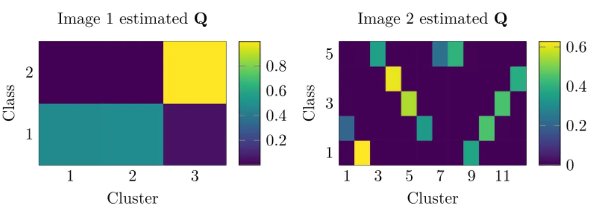
1.6. Estimated interaction matrix Q for Image 1 and Image 2 . . . . 42

1.7. Spectra used to generate the semi-synthetic image . . . 42

1.8. Semi-synthetic image. Panchromatic view of the hyperspectral image and ground-truth . . . 43

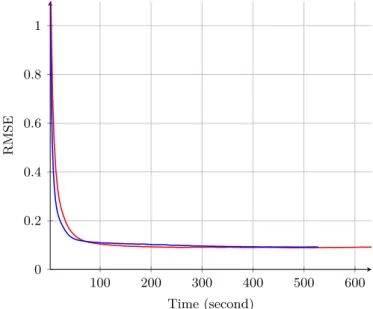
1.9. Evolution of RMSE of the sampled ˆA(t) _{matrix in function of the time for} the proposed model and Eches model . . . 43

1.10. Semi-synthetic image. Example of error map with the proposed model and with the Eches model . . . 44

1.11. Real MUESLI image. Dataset, clustering result and classification results . . . 45

1.12. Real MUESLI image. Classification accuracy measured with Cohen’s kappa as a function of the percentage of label corruption . . . 46

2.1. Structure of the cofactorization model . . . 56

2.2. Spectral unmixing concept (source US Navy NEMO). . . 61

2.3. Convergence of the various terms of objective function (representation learn-ing, clusterlearn-ing, classification, vTV, total). . . 66

2.4. Presentation of synthetic test image . . . 68

2.5. Spectra used as dictionary to generate the synthetic image . . . 69

2.6. Synthetic data: comparison of estimated abundance maps . . . 70

2.7. Synthetic data. Estimated classification maps . . . 72

2.8. AISA dataset presentation . . . 74

2.9. AISA data: spectra used as the dictionary M identified by the self-dictionary method. . . 76

2.10. AISA image. Estimated classification maps . . . 77

2.11. AISA dataset, comparison of estimated abundance maps of the 6 components 78 2.12. AISA data. Interpretation of results regarding the identified subclasses . . . . 80

3.1. Textures used to create synthetic dataset . . . 93

3.2. Synthetic dataset: abundance maps. . . 94

3.3. Synthetic dataset: segmentation map, color composition of the hyperspectral image, panchromatic image . . . 95

3.4. Image 1: estimated endmembers. . . 98

3.5. Image 1: abundance maps . . . .100

3.6. AVIRIS image: color composition of hyperspectral image and corresponding panchromatic image . . . 101

3.7. AVIRIS image: estimated endmembers . . . 103

3.8. AVIRIS image: estimated abundance maps . . . 105

1.1. Unmixing and classification results for all datasets. . . 40

2.1. Overview of notations. . . 57

2.2. Synthetic data: unmixing and classification results. . . 69

2.3. AISA data: information about classes. . . 75

2.4. AISA data: unmixing and classification results. . . 75

3.1. Image 1: quantitative results of unmixing (averaged over 10 trials). . . 97

3.2. Image 2: quantitative results of unmixing (averaged over 10 trials). . . 97

Au cours des dernières décennies, d’importants progrès ont été accomplis dans le domaine connu actuellement sous le nom d’intelligence artificielle ou d’apprentissage automatique. L’un des moteurs de cette révolution a été le développement d’algorithmes pour l’interpréta-tion automatique d’images. Il est par exemple possible de citer l’émergence dans les années 90 des machines à vecteurs de support (SVM), introduites d’abord pour la reconnaissance de chiffres manuscrits [BGV92]. Dans les années qui suivirent, les réseaux de neurones pro-fonds convolutionnels ont également été conçus pour résoudre ce même problème [LeC+98] et sont maintenant l’une des méthodes d’apprentissage les plus populaires.

L’attention croissante dont ont bénéficié ces technologies de pointe a amené les chercheurs et les utilisateurs à appliquer ces méthodes d’interprétation automatique dans de nombreux domaines d’application. En imagerie, de nombreuses méthodes d’analyse d’images ont été développées depuis la reconnaissance de chiffres manuscrits pour de nombreux cas d’appli-cation, par exemple la génération de cartes thématiques [LKC15], la segmentation d’images médicales [Ban08], la reconnaissance faciale [JL11], etc. Les méthodes de classification très populaires, telles que les SVMs ou les réseaux de neurones profonds, fournissent dorénavant de très bons résultats pour bon nombre de ces tâches.

Cependant, même si ces méthodes se sont révélées très efficaces, elles sont encore confron-tées à des problèmes délicats comme la grande dimension des données, le manque de don-nées labellisées, leur mauvaise labellisation ou encore le caractère multi-modale des classes considérées. Il a également été avancé que les résultats fournis par un classifieur, qui sont généralement un unique label par élément (un pixel, une image, . . .), sont quelque peu li-mités. En particulier, nombre de ces algorithmes restent très obscurs dans leur processus de décision. Les réseaux de neurones profonds sont par exemple souvent considérés comme des algorithmes “boîte noire”, bien que leur décision soit très précise [Cas16;Moo+17]. De plus, les méthodes de classification les plus utilisées ne recourent généralement pas à une modélisation du signal observé. Pour cette raison, il est difficile pour un spécialiste de guider l’interprétation par des connaissances experts sur la donnée observée.

Pour surmonter ces limitations, une alternative consiste à recourir à des approches fondées sur une modélisation des données. Les méthodes de classification sont principalement em-piriques, c’est-à-dire que la règle de décision est uniquement apprise à partir d’un ensemble d’exemples. Au contraire, les approches de type modélisation reposent sur une modélisation physique des données (signaux observés, images ou mesures). Par exemple, en imagerie mé-dicale, les modalités d’image sont généralement associées à un modèle physique du signal mesuré, dérivé des modalités particulières d’acquisition et d’un bruit spécifique [Cav+18b]. Parmi les approches basées sur des modèles, les méthodes d’apprentissage de représentation ont fait l’objet d’une attention importante.

Ces méthodes sont fondées sur l’hypothèse que les observations ne couvrent pas tout l’espace d’observation, mais sont en réalité contenues dans un sous-espace [BN08]. L’ap-prentissage de représentation vise à identifier ce sous-espace et à estimer la représentation de chaque observation dans celui-ci afin d’obtenir une représentation plus compacte, c’est-à-dire de dimension plus faible. Cette représentation de faible dimension est vue comme un ensemble de facteurs latents. Lorsque le modèle est construit à l’aide de connaissances a priori sur le domaine d’application, ces facteurs latents ont généralement une signification physique. Du point de vue de l’utilisateur, la possibilité de guider la méthode d’analyse afin d’estimer des paramètres spécifiques permet une interprétation beaucoup plus riche des résultats. Les produits annexes de ces méthodes d’apprentissage de représentation peuvent en effet présenter un grand intérêt. Par exemple, dans le cas du démélange hyperspectral, chaque vecteur de la base du sous-espace latent est associé à un matériau présent dans la scène observée [Bio+12].

Bien que la classification et l’apprentissage de représentation sont deux méthodes cou-ramment utilisées, elles n’ont que très rarement été envisagées conjointement. L’objectif de cette thèse est d’introduire le concept d’apprentissage de représentation et de classifica-tion conjoints. Les modèles unifiés développés sont ensuite testés sur un cas d’applicaclassifica-tion particulier qu’est l’analyse d’images hyperspectrales.

Structure du manuscrit

La première approche envisagée vise à mettre en place un nouveau modèle bayésien permet-tant d’estimer simultanément les classes et les représentations latentes. Pour cela, l’algo-rithme d’apprentissage de représentation considéré intègre une segmentation spatiale selon l’homogénéité des vecteurs de représentation latente. Dans l’approche proposée, le modèle de segmentation est complété de sorte à dépendre également des classes. La classification

est donc intégrée au modèle et exploite à la fois la donnée supervisée et la segmentation, qui intègre l’information bas-niveau, obtenant ainsi un classifieur robuste aux erreurs sur les données externes. L’algorithme fournit alors une description hiérarchique de l’image en termes de vecteurs latents, de segmentation spatiale et de classification thématique.

La deuxième approche considérée s’appuie sur la même description hiérarchique mais l’inférence est formulée comme un problème d’optimisation. La fonction de coût comprend alors trois termes principaux correspondant aux trois tâches considérées : l’apprentissage de représentation, la segmentation et la classification. Le problème obtenu s’apparente à un problème de cofactorisation de matrices avec un terme de segmentation liant les activa-tions des deux factorisaactiva-tions agissant respectivement comme modèle de représentation et de classification. Une solution de ce problème non-convexe et non-lisse est ensuite approchée à l’aide d’un algorithme de descente de gradient proximal alternée.

Le troisième travail réalisé vise à intégrer dans le processus de démélange hyperspectral une information spatiale complémentaire. L’originalité de la proposition réside dans le fait que l’information spatiale n’est pas introduite via un terme de régularisation mais comme un second terme d’attache aux données calculé à partir d’une image panchromatique de la scène. Ce modèle complète en particulier les deux approches précédentes en mettant en place une méthode de démélange permettant une bonne estimation des spectres élémentaires en capitalisant sur la méthode de cofactorisation développée précédemment.

Principales contributions

Chapitre 1. La principale contribution de ce chapitre réside dans l’introduction d’un cadre bayésien pour unifier les approches de modélisation physique bas-niveau et de classi-fication. Le modèle propose une utilisation de champs de Markov aléatoires pour relier tous les niveaux de modélisation afin de réaliser une estimation conjointe. La deuxième contri-bution est la conception d’une méthode de classification permettant de tenir compte des erreurs de labellisation dans l’ensemble d’apprentissage et de les corriger. Enfin, la dernière contribution réside dans le potentiel d’interprétation du modèle, notamment grâce à des produits annexes intéressants. En particulier, une des matrices estimées décompose cha-cune des classes en un ensemble de clusters chacun caractérisé par son vecteur d’abondance moyen. L’utilisateur peut ainsi analyser clairement la structure des données considérées. Chapitre 2. Un modèle de cofactorisation est utilisé pour développer un cadre unifié al-ternatif. Ce modèle diffère des autres modèles de cofactorisation principalement par le terme

de couplage proposé. Premièrement, il permet une interprétation riche des résultats avec à nouveau l’idée de décomposer les classes en un ensemble de clusters. Et deuxièmement, il permet de conserver une flexibilité entre les deux tâches à accomplir contrairement aux modèles précédemment proposés [ZL10] où le modèle introduit deux objectifs antagonistes au lieu d’objectifs coopératifs. La dernière contribution réside dans la proposition d’une méthode d’optimisation avancée pour minimiser la fonctionnelle proposée. En effet, un al-gorithme de minimisation proximale linéarisée alternée est utilisé pour résoudre le problème à la fois non convexe et non lisse, avec une garantie de convergence vers un point critique de la fonction objectif.

Chapitre 3. La principale contribution de ce chapitre est une nouvelle proposition pour enrichir directement le modèle de démélange spectral avec de l’information spatiale. Elle consiste à utiliser un terme supplémentaire d’attache aux données au lieu de recourir à des méthodes de régularisation. Ce nouveau modèle améliore les résultats du démélange. Mais plus important encore, le modèle produit une carte de clustering caractérisant différentes zones de l’image par leur signature spectrale et leur configuration spatiale. Cela permet d’obtenir une représentation compacte, complète et visuelle de la scène analysée. À notre connaissance, cette méthode introduit pour la première fois le concept de démélange spatial et spectral conjoint.

Over the last decades major progresses have occurred in the field of artificial intelligence. Many man-made activities have been successfully replaced by algorithms that are able to learn a given task directly from data. In particular, advances in image interpretation algo-rithms have been one of the driving force in this revolution. In the nineties, kernel methods, such as support vector machines (SVMs), were introduced firstly to identify handwritten digits [BGV92] and consisted in a major breakthrough. Specifically, SVMs highlighted non-probabilistic methods by proposing to minimize both a convex loss function while exploiting a set of labeled examples, and additional regularization terms to ensure a better separability of the classes. Following this trend, convolutional deep neural networks (CNN), which can automatically learn spatial features from the data, have become the top ranked methods for image recognition [LeC+98] and are now at the foundation of the most popular family of methods. Contrary to SVMs, the decision function of CNNs is a non-convex function composed of a sequence of differentiable operations. The parameters of this function are then optimized by minimizing a loss function, generally by using stochastic gradient descent. Although there is usually no convergence guarantee, CNNs manage to benefit from the huge quantity of available data to get state-of-the-art results.

The always increasing attention brought by these breakthrough technologies has pushed researchers and end-users to consider automatic interpretation methods in many fields of application such as remote sensing imaging [LKC15], medical imaging [Ban08], face recog-nition [JL11]. In particular, classification methods have received considerable attention. These methods aim at attributing a class to each elements of the analyzed dataset. These elements can take many forms ranging from simple pixels [Pla+09] to objects [ALL17] or images [KSH12]. The first step in classification generally consists in extracting a represen-tation of each element of the dataset either automatically as with CNNs [BCV13], or with handcrafted features [DT05;Low99;PB01]. Then, two main cases may come forth. The first case is unsupervised classification methods for which no additional information is available with the dataset. The concept behind these methods is generally to try to identify groups

of similar elements to which the same class is assigned. A typical case is a clustering task trying for example to separate organs in a medical image [Thi+14]. The second case occurs when a so-called training set is available with the data. This training set is a collection of observations that were classified manually by an expert. The set of examples is then used to train the classification model for the considered task. Many recent works have pointed out that the use of large training set is indeed very beneficial to the classification [KSH12; Mag+16].

However, even if supervised classification methods have proven to be very efficient, they still face challenging issues:

• The dimension of the observation is usually a major issue. The work of [Hug68] introduced the so-called curse of dimensionality. It showed in particular that statisti-cal methods made for low or moderate dimensional spaces do not adapt well to high dimensional spaces. The rate of convergence of the statistical estimation decreases when the dimension grows while the number of parameters to estimate simultane-ously increases, making the estimation of the model parameters very difficult [Don00]. Beyond a certain limit, the classification accuracy actually decreases as the number of features increases [Hug68]. These problems may arise when considering observa-tions with redundant information such as hyperspectral images [Cam+14] or video stream [Kar+14].

• The dependence to ground-truth data is also a recurrent limiting factor. The production of labeled data by experts is a critical work which is usually costly and time consuming. It is therefore common to be confronted with a lack of labeled data. For this reason, it is necessary to develop methods that leverage their dependence to GT data and are robust to overfitting [FM04; CFB08]. Semi-supervised methods are for example an attempt to deal with the lack of labeled data by using unlabeled data [CK05].

Another issue regarding the training data is the presence of incorrect labels [BF99; FV13]. This can be due to ambiguity regarding the set of classes or mistakes of the expert. In any case, the robustness to such labeling noise can be an interesting feature to characterize the performance of a classification algorithm [BG09].

• Handling multi-modal and/or composite classes with intrinsic intra-class vari-ability is also a recurrent issue [HT96a]. For instance, for a generic classification task, a class referred to as humans gathers distinct genders, or physical attributes.

When using too basic classifier, e.g. linear classifiers, it may actually be impossible to regroup the different modes in a single class [MP17].

It has also been argued that the outputs provided by a classifier, which are generally a unique label per elements (a pixel, an image,. . . ) of the dataset, are somehow limited. In particular, many of these algorithms remains very obscure in their decision process. First among them, CNN algorithms are nowadays often seen as black box algorithms although very accurate in their decision [Cas16; Moo+17]. Moreover, the most used classification methods are usually model-free, i.e., they are not based on a modeling of the observed signal. For this reason, when considering a specific task, it is difficult for a specialist to guide the interpretation by some prior knowledge.

To overcome this limitations, one alternative consists in resorting to model-based ap-proaches [Idi13]. Model-free classification methods are mostly empirical in the sense that the decision rule is only learned from a set of examples. On the contrary, model-based approaches rely on a modeling of the data (observed signals, images or measurements). For example, in medical imaging, image modalities are generally associated with a specific physics-based model of the measured signal, derived from the acquisition process and partic-ular noise corruption [Cav+18b]. Among model-based approaches, representation learning methods have received a considerable attention. Depending on the research community, representation learning has been referred to as dictionary learning methods [RPE12], ma-trix factorization [LS99], source separation [Bob+07], factor analysis [Cav+18b] or subspace learning [Li+15b]. These names denote representation learning methods differing mainly by the specific set of considered constraints enforced to ensure the physical interpretation of the data.

Representation learning – Representation learning is generally considered for modeling high-dimensional data. The main assumption underlying these methods is that the observa-tions do not span the whole observation space but are actually located in a subspace [BN08]. Representation learning aims at identifying this subspace and at estimating the represen-tation of each observation in this subspace to get a more compact represenrepresen-tation, i.e., of lower dimensionality [Ess+12]. This compact low-dimensional representation is a collection of latent factors. When the model is built in accordance with knowledge about the appli-cation field, these latent factors usually carry some physical meaning [El +06]. From the end-user point-of-view, the possibility to guide the analysis method in order to estimate specific parameters offers a richer interpretation of the results. The byproducts provided by representation learning methods can indeed be of the highest interest. For example, in the

case of hyperspectral unmixing, each vector of the basis spanning the subspace is identified to a material present in the observed scene [Bio+12].

However, a major drawback of this family of methods is the complexity of the targeted results. First, generally, representation learning results in very challenging estimation prob-lems. Indeed, physics-based models often introduce non-convex problems [RCP14;Bob+15]. When considering optimization frameworks, such problems remain difficult to tackle and it is generally impossible to ensure convergence to a global optimum of the objective function. Some advanced methods can at least guarantee convergence to some local optimum [BST14; WYZ19]. However, the quality of the results then highly depends on the possibility to pro-pose an initialization point close enough to the solution. Additionally to the non-convexity issues, representation learning commonly includes non-smooth terms because of the con-straints inherent to compact representations, such as sparsity, or the constraint imposed on the search space, such as non-negativity constraints. One possibility to deal with this second issue is to resort to advanced optimization tools such as proximal methods [CP11].

To avoid estimation problems related to non-convexity or non-smoothness, one possibil-ity is to resort to Markov chain Monte Carlo (MCMC) methods [Per+12;Per+15;EDT11]. Contrary to optimization methods, these methods use a Bayesian modeling of the prob-lem. Each estimated variable is assigned a prior distribution model and the main concept of MCMC algorithm is to generate samples according to the joint posterior distribution [RC04; Bro+11]. The Bayesian estimators of the parameters of interest can then be approximated using these samples. Besides, these samples can be used to provide a full description of the posterior distribution of interest, beyond a simple point estimation (e.g., maximum a poste-riori estimators). For example, it gives the possibility to provide confidence sets. Moreover, the convexity of the problem is not required to ensure convergence of the estimation. Never-theless, one major drawback of these methods is that, even if the convergence is guaranteed, it is not possible to predict when convergence will be reached. MCMC methods thus allow users to deal with complex settings but fail in many cases to scale to real practical problems due to the extensive computational burden needed to get the results [Per+15].

Additionally to estimation problems, another recurrent issue is the difficulty to include exogenous data into a representation learning task [MBP12]. As discussed previously, super-vised classification methods are nowadays considered the most efficient methods to extract information from data. It could be argued that this efficiency comes from the ability of these methods to incorporate the information coming from the examples provided by the user. Unfortunately it would be tedious to copy such a process to representation learning methods. The problem comes in particular from the difficulty to gather handmade

exam-ples. Most of the time it is impossible for experts to estimate the expected output from the image. In order to get a rich output and to benefit from exogenous data, a possibility is to consider the development of joint methods [Mai+09]. Such methods have the advantages to solve the problem of high-dimensional data for the classification by producing meaningful low-dimensional representations. Besides, some of the information contained in the classi-fication training set is likely to be transfered to the representation learning problem and help solve it. The development of image analysis methods proposing a joint classification and representation learning approach is one of the key interest of this manuscript. For this reason it is interesting to get a closer look at the works which have already proposed in the literature to conduct classification and representation learning jointly.

Joint classification and representation learning – Many of the works on joint ap-proaches have been published in the dictionary learning community, in which representation learning is actually referred to as dictionary learning [AEB06;RBE10]. In these approaches, it is usual to identify the subspace containing the observations by inferring a so-called dic-tionary. This dictionary is a collection of elementary vectors, referred to as atoms, spanning the representation subspace. The idea of supervised dictionary learning has been popu-larized in particular by the work of Mairal et al. [Mai+09; MBP12]. The core concept of supervised dictionary learning is to develop models in which the dictionary is built for a specific classification application. The dictionary should both demonstrate a reconstruc-tion ability and a discriminative ability. The Discriminative K-SVD (DKSVD) described in [ZL10] proposes for instance to directly consider an optimization problem composed of a data fitting term and a linear classification term. Authors performed a face recognition task with a two-step algorithm including a training step to learn a relevant dictionary followed by an inference step to classify unknown samples using the learned representation. This work was implemented for the same task in [JLD11] with the difference that the learned dictionary promoted the use of different dictionary atoms for each class.

Going further, some works aimed at recovering specific dictionaries. These class-specific dictionaries are learned to ensure a good discrimination of the classes. To solve an object classification problem, the authors of [FRZ18] proposed for example to promote structural incoherence between the dictionaries of the various classes using an orthogonality penalization between the dictionary atoms. Further attempts were also made to exploit the training set of the classification task more thoroughly. For example in [CNT11], all the pixels of the training set were used as dictionary and a sparse representation of the unknown pixels was then inferred. Moreover, since dictionary atoms were associated with a

class label, the contribution of each class for the reconstruction of each pixel was computed using a reconstruction error metric. Finally, pixels were assigned to the class contributing the most to their reconstruction.

Broadly speaking, the idea of performing two complementary tasks simultaneously has already been investigated and has resulted into a family of models called cofactorization models [HDD13]. In particular, joint representation learning and classification can be cast as a cofactorization problem. Both tasks are interpreted as individual factorization prob-lems and a coupling term and/or constraints between the dictionaries and coding matrices associated with the two problems are then introduced. These cofactorization-based models have proven to be highly efficient in many application fields, e.g., for text mining [WB11], music source separation [Yoo+10], and image analysis [YYI12;AM18].

A common thread found in all the aforementioned works is the perspective chosen to tackle the problem of joint classification and representation learning. The main objective is generally to design a classification method and the representation learning process is only considered as a mean to this end [BCV13]. More specifically, representation learning is used to solve the statistical issues occurring with high-dimensional data. It operates as a dimensionality reduction method aiming at providing the best low-dimensional representa-tion for the classificarepresenta-tion [LC09]. Such perspective is very likely to be detrimental to the representation learning process since it appears as secondary. Indeed, the discriminative and reconstruction abilities of the dictionary are often seen as adversarial in these models. The work presented in this manuscript gathers new strategies to tackle the problem of joint approaches. The main objective is to provide truly cooperative joint representation learning and classification methods by considering a coherent hierarchical modeling using both methods. To illustrate the relevance of the methods proposed in this manuscript, an application to hyperspectral image analysis has been considered through the dual scope of spectral unmixing and classification.

Analysis of hyperspectral images – Hyperspectral images are particularly well-suited to be studied with representation learning methods due to the high dimension of the pixels of this specific modality of images. As a reminder, conventional color imaging has been designed in order to mimic human eye and, for this reason, these images are composed of three bands corresponding each to the reflectance measured for the blue, green and red wavelengths. However the spectral information contained in such an image is eventually very limited. Indeed, the reflectance, defined as the fraction of incident electromagnetic power that is reflected, varies for each wavelength depending on the electromagnetic

prop-erties of the observed scene [SM02;Lan02]. It is actually possible to measure this reflectance spectrum for hundreds of specific wavelength and thus obtain a very accurate electromag-netic characterization of the scene [Pla+09]. In the case of hyperspectral imaging, hundreds of measurements are performed in order to get a fine sampling of the reflectance spectrum of the area underlying each pixel. Moreover, measurements are not limited to the visible domain but usually include a larger part of the electromagnetic spectrum, e.g., the infrared domain [Van+93].

The study of the electromagnetic properties of matter has shown that every material can actually be characterized by a specific reflectance spectrum [Hap93]. Unfortunately, due to the limited spatial resolution of the hyperspectral sensors, the area described by a given pixel usually includes a collection of materials. The result is the creation of mixels, i.e., pixels representing a mixture of elementary reflectance spectra of pure material, usually referred to as endmembers, as shown in Figure .1. Spectral unmixing aims at identify-ing these endmembers and estimatidentify-ing the proportions of each pure material inside each pixel [Bio+12]. This method of interpretation actually fits in the family of representation learning methods where the learned representation subspace is the subspace spanned by the identified endmembers and the latent representation is the vector of proportions of pure materials, generally called abundance vector.

Spectral unmixing is widely-used to interpret hyperspectral images particularly because of the richness of the data that allows a physical interpretation of the results. Moreover, the high dimension and high redundancy of the hyperspectral pixels may make it diffi-cult to perform a classification [Cam+14; Fau+13]. Therefore, it is often necessary to use dimensionality reduction methods prior to classification [ZD16;LFG17].

Bearing in mind the aim to propose joint representation learning and classification meth-ods, reviewing the previous works that attempted to link both methods in the specific context of hyperspectral imaging appeared of great interest. The frameworks proposed in the literature for a joint use of spectral unmixing and classification are generally based on a sequential use of the two approaches. The most simple way to implement a sequential ap-proach is to use spectral unmixing as a feature extraction method. The abundance vectors can be used as feature vectors for the classification which is then performed with the help of a conventional classifier, as done with SVM in [LC09;Vil11;Dóp+11;Dóp+12] or with a deep neural network in [Ala+17]. Spectral unmixing as feature extraction method presents the benefit of reducing drastically the dimension as well as proposing features with physical meaning. However, these features remain rather simple and do not maximize the separabil-ity of the classes. Additionally, spectral unmixing does not profit at all from any information

0.5 1 1.5 2 2.5 0 0.2 0.4 wavelength (µm) reflectance Components of spectrum

Figure .1.: Hyperspectral images are images with a fine spectral resolution. The measured reflectance spectrum of a pixel is explained as a mixture elementary components each rep-resenting a specific material.

coming from the classification. The classification map is actually the only considered result and spectral unmixing is only a tool to help the classification.

Spectral unmixing has also been used to improve classification results, more precisely to perform sub-pixel mapping [Vil+11b; Vil+11a]. The main idea is to identify mixed pixels, i.e., pixels representing areas containing several classes, and then split these pixels to increase the spatial resolution. Spectral unmixing is used to assign classes to the newly created pixels. For example, if unmixing shows that a pixel contains 80% of vegetation and 20% of soil, 80% of the underlying new pixels are assigned to class vegetation and 20% to soil. A major limitation to these methods is that an endmember has to be equivalent to a class.

Nevertheless, several works used this assumption of equivalence between classes and end-members. In the semi-supervised classification methods proposed in [Dóp+14;Li+15a], the spectral unmixing method was used directly as a classifier where the abundance vectors were directly interpreted as vectors collecting the probabilities to belong to each of the classes. Spectral unmixing was used side-by-side with a multinomial logistic regression (MLR). Be-sides, the two classifiers were used in an active learning method combining them to increase the size of the training set by generating labels to identified informative pixels.

focusing on classification problems with small training sets, introduced the idea of using all the pixels of the training set as endmembers. A sparse spectral unmixing method was then used to infer the abundance vectors. Finally, for each unlabeled pixel the predominant endmember was identified and its class was attributed the unlabeled pixel.

The same authors also proposed in [And+19] a classification method based on a decision fusion framework where the results of two classifiers were merged with the help of Markov or conditional random fields. The first classifier was a conventional MLR classifier and the second was similar to the one of [And+16] with the difference that fractional abundances were computed by summing all the abundances of endmembers of a same class yielding a probability vector to belong to each of the classes.

Another family of methods makes the link between classification and spectral unmixing by assuming that all the pixels of a given class live in a class-specific subspace. In particular, the early work [LBP12] proposed a segmentation method combining projection in class-specific subspaces with a MLR algorithm. From an unmixing point of view, this assumption also means that it is possible to use class-specific endmember matrices. Authors of [Sun+17] thus proposed to use a training set to estimate an endmember matrix for each class, then to concatenate all these endmember matrices to get a global endmember matrix and finally to use a sparse spectral unmixing method and classification method based on fractional abundances to get both unmixing results and classification results. The idea developed in these two latter works were combined in [Xu+19] in which the authors proposed to evaluate class-specific endmember matrices and the identified subspaces were then used to create a transformation function applied to the data, then used to feed a MLR algorithm.

This brief overview shows that very few attempts have been conducted to propose a joint spectral unmixing and classification method. Moreover, these methods generally tackle the problem by using the two approaches sequentially and, in most cases, with the final idea to get an improved classification method. Convinced that the representation learning results are as worthy of consideration as classification results for an end-user, the work presented in this manuscript is an attempt to propose truly joint representation learning and classification methods. The aim of these methods is to provide a hierarchical description of the considered data.

The work presented in this manuscript has been carried out within the Signal and Com-munications group of the Institut de Recherche en Informatique de Toulouse. This thesis was funded by the Centre National d’Études Spatiales (CNES) and Région Occitanie.

Structure of the manuscript

Chapter 1 introduces a hierarchical Bayesian model, inspired by [EDT11], to jointly perform low-level modeling and supervised classification. The low-level modeling intends to extract the latent structure of the data whereas classification is considered as a high-level modeling. These two stages of the hierarchical model are linked through a clustering stage which aims at identifying groups of pixels with similar latent representation. A Markov random field (MRF) is then used to ensure a spatial regularity of the cluster labels and a coherence with classification labels. The final stage used for classification exploits a set of possibly corrupted labeled data provided by the end-user. The parameters of the overall Bayesian model are estimated using a Markov chain Monte Carlo (MCMC) algorithm in the specific case where the image is an hyperspectral image and the low-level modeling is a spectral unmixing model.

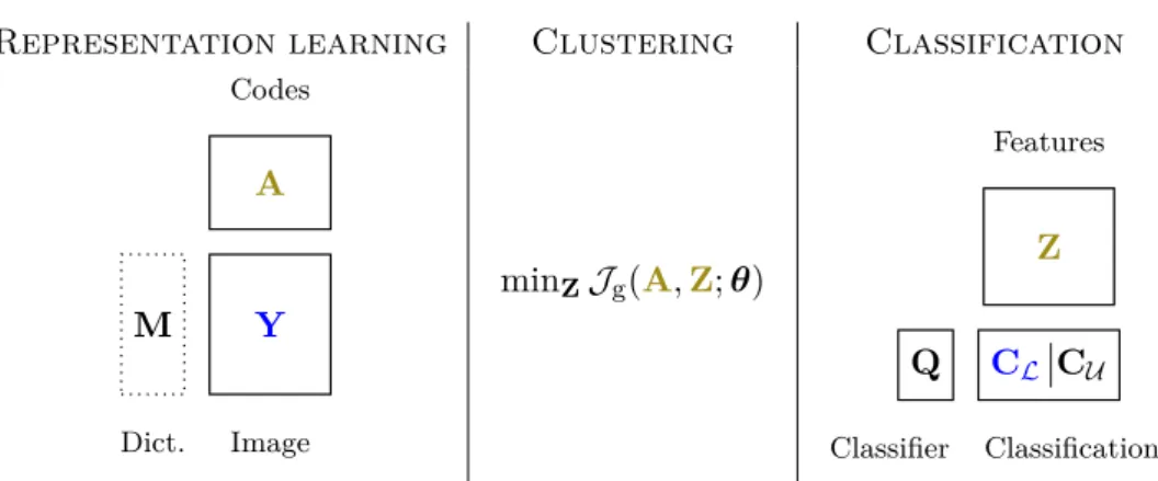
Chapter 2 considers a different approach by using of a cofactorization model. The repre-sentation learning task and the classification task are both modeled as factorization matrix problems. A coupling term is then introduced to enable a joint estimation. Based on the same idea developed in model of Chapter 1, the coupling term is interpreted as a clus-tering task performed on the low-dimensional representation vectors. Finally, the cluster attribution vectors are used as features vectors for classification. The overall non-smooth, non-convex optimization problem is solved using a proximal alternating linearized minimiza-tion (PALM) algorithm ensuring convergence to a critical point of the objective funcminimiza-tion. The quality of the obtained results is finally assessed on synthetic and real data for the analysis of hyperspectral image using spectral unmixing and classification.

Chapter 3 intends to enrich the previous model by adding spatial information. In the previous models, the spatial information is only exploited through regularization terms such as Potts-MRF or total variation regularization. With this mechanism, spatial information is introduced at a late stage in an indirect manner. To introduce a more direct spatial information, a cofactorization model with two data fitting terms is considered. The first term is a spectral mixture model based on the hyperspectral image and thus accounts for the spectral information. The second term is a representation learning model based on an image aggregating the spatial information. This image can be computed from a panchromatic image, e.g., by extracting spatial features or by concatenating the neighborhood of each pixel. The coupling term is again a clustering task identifying groups of pixels with similar spectral and spatial signatures. The resulting model performs an unsupervised unmixing

task and could be merged with the model of Chapter2to derive a richer supervised model.

Main contributions

Chapter 1. The main contribution of this chapter lies in the introduction of a Bayesian framework to unify representation learning and classification approaches. The model pro-poses a resourceful use of MRF to link all the levels of the model to conduct a joint esti-mation. The second contribution is the design of a classification method robust to labeling errors in the training set. The method additionally proposes a correction of erroneous la-bels. Finally, the last contribution is in the potential of interpretation of the results due to meaningful byproducts. In particular, a matrix decomposing the classes into a collection of clusters is estimated and each of these clusters are characterized by their mean abundance vector. These byproducts allow the user to clearly visualize the structure of the considered data.

Chapter 2. A cofactorization model is used to develop another unified framework for representation learning and classification. This model differs from other cofactorization model mainly by the proposed coupling term. Firstly, it allows a rich interpretation of the results with again the idea of decomposing classes in a collection of clusters. And sec-ondly, it keeps flexibility between the two tasks at hand, contrary to previous models such as DKSVD [ZL10] where the model introduces two adversarial goals instead of coopera-tive ones. The final contribution lies in the proposition of a powerful optimization method dedicated to the criterion to be minimized. Indeed, a proximal alternating linearized mini-mization algorithm (PALM) is used to solve the non-convex, non-smooth problem at hand with guarantee of convergence to a critical point of the objective function.

Chapter 3. The main contribution of this chapter is a new proposition to enrich spectral mixture model with spatial information directly using an additional data fitting term instead of resorting to regularization methods. This new model tends to improve the results of the unmixing process. But more importantly, the model produces a segmentation map identifying several areas by their spectral signature and their spatial pattern. We actually obtain a very compact, complete and visual representation of the analyzed scene. Up to our knowledge, this method introduces the new concept of joint spatial-spectral unmixing.

Submitted

[Lag+19c] A. Lagrange, M. Fauvel, S. May, J. Bioucas-Dias, and N. Dobigeon. “Matrix Cofactorization for Joint Representation Learning and Supervised Classifica-tion – ApplicaClassifica-tion to Hyperspectral Image Analysis”. In: arXiv:1902.02597 [cs, eess] (Feb. 2019). arXiv:1902.02597 [cs, eess] (cit. on p.49).

[Lag+19e] A. Lagrange, M. Fauvel, S. May, and N. Dobigeon. “Matrix Cofactorization for Joint Spatial-Spectral Unmixing of Hyperspectral Images”. In: arXiv:1907.08511 [cs, eess] (July 2019). arXiv:1907.08511 [cs, eess](cit. on p. 83).

International journals

[Lag+19d] A. Lagrange, M. Fauvel, S. May, and N. Dobigeon. “Hierarchical Bayesian Image Analysis: From Low-Level Modeling to Robust Supervised Learning”. In: Patt. Recognition 85 (2019), pp. 26–36 (cit. on p.19).

International conferences

[Lag+18] A. Lagrange, M. Fauvel, S. May, and N. Dobigeon. “A Bayesian Model for Joint Unmixing and Robust Classification of Hyperspectral Images”. In: Proc. IEEE Int. Conf. Acoust., Speech and Signal Process. (ICASSP). IEEE, 2018, pp. 3399–3403 (cit. on pp.19,55).

[Lag+19b] A. Lagrange, M. Fauvel, S. May, J. M. Bioucas-Dias, and N. Dobigeon. “Ma-trix Cofactorization for Joint Unmixing and Classification of Hyperspectral Images”. In: Proc. European Signal Process. Conf. (EUSIPCO). Sept. 2019 (cit. on p.49).

National conferences

[Lag+17] A. Lagrange, M. Fauvel, S. May, and N. Dobigeon. “Un Modèle Bayésien Pour Le Démélange, La Segmentation et La Classification Robuste d’images Hyper-spectrales”. In: Actes du Colloque GRETSI. 2017, pp. 1–4 (cit. on p.19). [Lag+19a] A. Lagrange, M. Fauvel, S. May, J. M. Bioucas-Dias, and N. Dobigeon.

“Co-factorisation de Matrices Pour Le Démélange et La Classification Conjoints d’Images Hyperspectrales”. In: Actes du Colloque GRETSI. Aug. 2019 (cit. on p.49).

Publications prior to the Ph.D. work

[Cam+16] M. Campos-Taberner, A. Romero-Soriano, C. Gatta, G. Camps-Valls, A. La-grange, B. Le Saux, A. Beaupère, A. Boulch, A. Chan-Hon-Tong, S. Herbin, H. Randrianarivo, M. Ferecatu, M. Shimoni, G. Moser, and D. Tuia. “Processing of Extremely High-Resolution LiDAR and RGB Data: Outcome of the 2015 IEEE GRSS Data Fusion Contest - Part A: 2-D Contest”. In: IEEE J. Sel. Topics Appl. Earth Observations Remote Sens. 9.12 (Dec. 2016), pp. 5547– 5559.

[Lag+15] A. Lagrange, B. Le Saux, A. Beaupere, A. Boulch, A. Chan-Hon-Tong, S. Herbin, H. Randrianarivo, and M. Ferecatu. “Benchmarking Classification of Earth-Observation Data: From Learning Explicit Features to Convolutional Networks”. In: Proc. IEEE Int. Conf. Geosci. Remote Sens. (IGARSS). IEEE, 2015, pp. 4173–4176.

[LFG17] A. Lagrange, M. Fauvel, and M. Grizonnet. “Large-scale feature selection with Gaussian mixture models for the classification of high dimensional remote sens. images”. In: IEEE Trans. Comput. Imag. 3.2 (2017), pp. 230–242 (cit. on pp.11,

Hierarchical Bayesian model for

joint classification and spectral

unmixing

Contents

1.1. Introduction (in French) . . . 20

1.2. Introduction . . . 21

1.3. Hierarchical Bayesian model . . . 23

1.3.1. Low-level interpretation . . . 24 1.3.2. Clustering . . . 25 1.3.3. High-level interpretation . . . 27 1.4. Gibbs sampler . . . 29 1.4.1. Latent parameters . . . 30 1.4.2. Cluster labels . . . 30 1.4.3. Interaction matrix . . . 31 1.4.4. Classification labels . . . 32

1.5. Application to hyperspectral image analysis . . . 33

1.5.1. Low-level model . . . 34 1.5.2. Clustering . . . 35

1.6. Experiments . . . 37

1.6.1. Synthetic dataset . . . 37 1.6.2. Real hyperspectral image . . . 44

1.7. Conclusion and perspectives . . . 47

1.1. Introduction (in French)

Dans le contexte de l’interprétation d’images, de nombreuses méthodes ont été dévelop-pées pour extraire l’information utile. Parmi ces méthodes, les modèles génératifs ont reçu une attention particulière du fait de leurs solides bases théoriques, mais aussi de la facilité d’interprétation des modèles estimés en comparaison des modèle discriminatifs, comme les réseaux de neurones profonds. Ces méthodes sont basées sur une modélisation statistique explicite des données. Ils permettent la construction de modèles dédiés pour chaque appli-cation [WG13], ou bien la construction de modèles plus génériques comme les modèles de mélange de gaussiennes pour la classification [Ker14]. L’utilisation de modèles spécialisés ou génériques représente deux approches différentes pour obtenir une description interprétable des données. Par exemple, lorsqu’on analyse des images, les modèles spécialisés visent à reconstituer la structure latente (potentiellement basée sur un modèle physique) de cha-cune des mesures pixeliques [DTC08] tandis que la classification produit une information haut-niveau réduisant la caractérisation des pixels à un unique label [FCB12].

La principale contribution de ce chapitre réside dans la définition d’un nouveau mo-dèle bayésien développant un cadre unifié pour réaliser classification et modélisation des structures latentes de manière jointe. Ce modèle a l’avantage d’estimer des descriptions bas-niveau et haut-niveau cohérentes de l’image en réalisant une analyse hiérarchique de l’image. De plus, il est possible d’espérer une amélioration des résultats de chacune des méthodes grâce à la complémentarité des approches. En particulier, l’utilisation de données labellisées n’est plus limitée à l’analyse haut-niveau, i.e., la classification. Il est également possible d’informer l’analyse bas-niveau, c’est-à-dire, la modélisation des structures latentes, qui profite en général mal de telles informations a priori. D’autre part, les variables latentes de la modélisation bas-niveau peuvent être utilisées comme descripteurs pour la classifica-tion. Un effet collatéral direct est la réduction de dimension explicite réalisée sur les données avant la classification [JL98]. Enfin, le modèle hiérarchique introduit permet de rendre la classification robuste à la corruption des labels d’entraînement. En effet, les performances d’une méthode de classification supervisée peuvent se dégrader si ces derniers ne sont pas entièrement fiables comme c’est souvent le cas puisque ces labels sont estimés par des experts humains pouvant commettre des erreurs. Pour cette raison, le problème de développer des méthodes de classification robustes aux erreurs de labellisation a été largement considéré dans la communauté [BG09;Pel+17]. S’inscrivant dans ce cadre, le modèle proposé tient

explicitement compte de la présence de labels corrompus.

L’interaction entre les modèles bas-niveau et haut-niveau est géré par l’utilisation de champs de Markov aléatoires (MRF) non-homogènes [Li09]. Les MRFs sont des modèles pro-babilistes largement utilisés pour décrire des interactions spatiales. C’est pourquoi, lorsqu’ils sont utilisés comme a priori dans une modélisation bayésienne, ils sont tout à fait adaptés pour capturer les dépendances spatiales entre les structures latentes des images [ZBS01; Tar+10;And+19;Che+17]. Le modèle proposé inclut lui deux instances de MRFs assurant (i) la cohérence entre les modélisations bas-niveau et haut-niveau, (ii) la cohérence avec les labels fournis par les experts comme donnée d’entraînement et (iii) une régularité spatiale. La suite de ce chapitre est organisée de la manière suivante. La Section 1.3 présente le modèle bayésien hiérarchique proposé comme cadre unifié pour l’interprétation bas-niveau et haut-niveau d’images. Une méthode de Monte Carlo par chaîne de Markov est explicitée dans la Section1.4pour permettre l’échantillonnage selon la loi postérieur jointe des paramètres du modèle. Ensuite, une instance particulière du modèle est considérée dans la Section1.5

où, en se recentrant sur le cas d’étude de ce manuscrit, des images hyperspectrales sont analysées à la fois du point de vue du démélange et de la classification. La Section 1.6

présente les résultats obtenus avec la méthode proposée et les compare à ceux obtenus avec des méthodes établies en utilisant des données synthétiques puis réelles. Finalement, la Section1.7 conclut ce chapitre et ouvre quelques perspectives de recherche dans la suite de ce travail.

1.2. Introduction

In the context of image interpretation, numerous methods have been developed to extract meaningful information. Among them, generative models have received a particular atten-tion due to their strong theoretical background and the great convenience they offer in term of interpretation of the fitted models compared to some model-free methods such as deep neural networks. These methods are based on an explicit statistical modeling of the data which allows very task-specific model to be derived [WG13], or either more general models to be implemented to solve generic tasks, such as Gaussian mixture models for classifica-tion [Ker14]. Task-specific and classificaclassifica-tion-like models are two different ways to reach an interpretable description of the data with respect to a particular applicative issue. For instance, when analyzing images, task-specific models aim at recovering the latent (possibly physics-based) structures underlying each pixel-wise measurement [DTC08] while classifi-cation provides a high-level information, reducing the pixel characterization to a unique

label [FCB12].

The contribution of this chapter lies in the derivation of a unified Bayesian framework able to perform classification and latent structure modeling jointly. This framework has the primary advantage of recovering consistent high and low level image descriptions, explicitly conducting hierarchical image analysis. Moreover, improvements in the results associated with both methods may be expected thanks to the complementarity of the two approaches. In particular, the use of ground-truthed training data is not limited to driving the high level analysis, i.e., the classification task. Indeed, it also makes it possible to inform the low level analysis, i.e., the latent structure modeling, which usually does not benefit well from such prior knowledge. On the other hand, the latent modeling inferred from each data as low level description can be used as features for classification. A direct and expected side effect is the explicit dimension reduction operated on the data before classification [JL98]. Finally, the proposed hierarchical framework allows the classification to be robust to corruption of the ground-truth. As mentioned previously, performance of supervised classification may be questioned by the reliability in the training dataset since it is generally built by human expert and thus probably corrupted by label errors resulting from ambiguity or human mistakes. For this reason, the problem of developing classification methods robust to label errors has been widely considered in the community [BG09; Pel+17]. Pursuing this objective, the proposed framework also allows training data to be corrected if necessary.

The interaction between the low and high level models is handled by the use of non-homogeneous Markov random fields (MRF) [Li09]. MRFs are probabilistic models widely-used to describe spatial interactions. Thus, when widely-used to derive a prior model within a Bayesian approach, they are particularly well-adapted to capture spatial dependencies between the latent structures underlying images [ZBS01;Tar+10; And+19]. For example, Chen et al. [Che+17] proposed to use MRFs to perform clustering. The proposed framework incorporates two instances of MRF, ensuring (i) consistency between the low and high level modeling, (ii) consistency with external data available as prior knowledge and (iii) a more classical spatial regularization.

The remaining of the chapter is organized as follows. Section1.3presents the hierarchical Bayesian model proposed as a unifying framework to conduct low-level and high-level image interpretation. A Markov chain Monte Carlo (MCMC) method is derived in Section1.4 to sample according to the joint posterior distribution of the resulting model parameters. Then, focusing on the problem at hand in this manuscript, a particular and illustrative instance of the proposed framework is presented in Section1.5where hyperspectral images are analyzed under the dual scope of unmixing and classification. Section1.6presents the results obtained

with the proposed method and compares them to the results of well-established methods using synthetic and real data. Finally, Section 1.7 concludes the chapter and opens some research perspectives to this work.

1.3. Hierarchical Bayesian model

In order to propose a unifying framework offering multi-level image analysis, a hierarchical Bayesian model is derived to relate the observations and the task-related parameters of interest. This model is mainly composed of three main levels. The first level, presented in Section 1.3.1, takes care of a low-level modeling achieving latent structure analysis. The second stage then assumes that data samples (e.g., resulting from measurements) can be divided into several statistically homogeneous clusters through their respective latent struc-tures. To identify the cluster memberships, these samples are assigned discrete labels which are a priori described by a non-homogeneous Markov random field (MRF). This MRF com-bines two terms: the first one is related to the potential of a Potts-MRF to promote spatial regularity between neighboring pixels; the second term exploits labels from the higher level to promote coherence between cluster and classification labels. This clustering process is de-tailed in Section1.3.2. Finally, the last stage of the model, explained in Section1.3.3, allows high-level labels to be estimated, taking advantage of the availability of external knowledge as ground-truthed or expert-driven data, akin to a conventional supervised classification task. The whole model and its dependences are summarized by the directed acyclic graph in Figure1.1. Y υ A θ z β1 Q ω β2 η cL Observations Low-level

task Clustering High-level_task

Figure 1.1.: Directed acyclic graph of the proposed hierarchical Bayesian model. (User-defined parameters appear in dotted circles and external data in squares).

1.3.1. Low-level interpretation

The low-level task aims at inferring P R-dimensional latent variable vectors ap (∀p ∈ P ,

{1, . . . , P }) appropriate for representing P respective d-dimensional observation vectors yp

in a subspace of lower dimension than the original observation space, i.e., R ≤ d. The task may also include the estimation of the function or additional parameters of the function relating the unobserved and observed variables. By denoting Y = [y1, . . . ,yP] and A =

[a1, . . . ,aP] the d×P - and R×P - matrices gathering respectively the observation and latent

variable vectors, this relation can be expressed through the general statistical formulation Y|A, υ ∼ Ψ (Y; flat(A) , υ) , (1.1) where Ψ(·, υ) stands for a statistical model, e.g., resulting from physical or approximation considerations, flat(·) is a deterministic function used to define the latent structure and υ are possible additional nuisance parameters. In most applicative contexts aimed by this work, the model Ψ(·) and function flat(·) are separable with respect to the measurements assumed to be conditionally independent, leading to the factorization

Y|A, υ ∼

P Y p=1

Ψ (yp; flat(ap) , υ) . (1.2)

It is worth noting that this statistical model will explicitly lead to the derivation of the particular form of the likelihood function involved in the Bayesian model.

The choice of the latent structure related to the function flat(·) is application-dependent and can be directly chosen by the end-user. A conventional choice consists in considering a linear expansion of the observed data yp over an orthogonal basis spanning a space whose

dimension is lower than the original one. This orthogonal space can be a priori fixed or even learnt from the dataset itself, e.g., leveraging on popular nonparametric methods such as principal component analysis (PCA) [FCB06]. In such case, the model (1.1) should be interpreted as a probabilistic counterpart of PCA [TB99] and the latent variables ap

would correspond to factor loadings. Similar linear latent factors and low-rank models have been widely advocated to address source separation problems, such as nonnegative matrix factorization [CNJ09]. As a typical illustration, by assuming an additive white and centered Gaussian statistical model Ψ(·) and a linear latent function flat(·), the generic model (1.2)