1
Title
1
RIVER FLOOD MAPPING IN URBAN AREAS COMBINING RADARSAT-2 DATA AND FLOOD 2
RETURN PERIOD DATA 3
4
Author names and affiliations
5
Marion Tanguy a*, Karem Chokmani a, Monique Bernier a, Jimmy Poulin a, Sébastien Raymond a 6
a
Institut National de la Recherche Scientifique, Centre Eau Terre Environnement, 490 rue de la
7
Couronne, G1K 9A9 Québec (QC) Canada.
8
E-mail: [email protected] (K.C); [email protected] (M.B);
9
[email protected] (J.P); [email protected] (S.R)
10
11
* Corresponding author: Tel: +1 1418 654 2530 – 4466
12
E-mail: [email protected] (M. Tanguy) 13 14 15 16 17 18 19 20 21 22
2
Abstract
23 24
Near-real-time flood maps are essential to organize and coordinate emergency services' 25
response actions during flooding events. Thanks to its capacity to acquire synoptic and detailed 26
data during day and night, and in all weather conditions, Synthetic Aperture Radar (SAR) 27
satellite remote sensing is considered one of the best tools for the acquisition of flood mapping 28
information. However, specific factors contributing to SAR backscatter in urban environments, 29
such as shadow and layover effects, and the presence of water surface–like radar response 30
areas, complicate the detection of flood water pixels. This paper describes an approach for 31
near-real-time flood mapping in urban and rural areas. The innovative aspect of the approach is 32
its reliance on the combined use of very-high-resolution SAR satellite imagery (C-Band, HH 33
polarization) and hydraulic data, specifically flood return period data estimated for each point of 34
the floodplain. This approach was tested and evaluated using two case studies of the 2011 35
Richelieu River flood (Canada) observed by the very-high-resolution RADARSAT-2 sensor. In 36
both case studies, the algorithm proved capable of detecting flooding in urban areas with good 37
accuracy, identifying approximately 87% of flooded pixels correctly. The associated false 38
negative and false positive rates are approximately 14%. In rural areas, 97% of flooded pixels 39
were correctly identified, with false negative rates close to 3% and false positive rates between 40
3% and 35%. These results highlight the capacity of flood return period data to overcome 41
limitations associated with SAR-based flood detection in urban environments, and the relevance 42
of their use in combination with SAR C-band imagery for precise flood extent mapping in urban 43
and rural environments in a crisis management context. 44
45
Keywords:Flood mapping; Synthetic Aperture Radar, C-Band; Flood return period 46
3
1. Introduction
48 49
The capacity of spaceborne Synthetic Aperture Radar (SAR) remote sensing for near-real-time 50
flood detection and mapping has been demonstrated by numerous studies over the last decade 51
(Henry et al., 2006, Greifeneder et al., 2014, Schumann et al., 2011; Schumann et al., 2012; 52
Pulvirenti et al., 2014). Many civil protection organizations now use airborne and satellite SAR 53
imagery to support the development of assistance plans to reduce human and material 54
consequences of flooding events (Bhatt et al., 2016 ; Boni et al., 2009 ; Kussul et al., 2014 ; 55
Martinis et al., 2015 ; Pulvirenti et al., 2013 ; Zhang et al., 2002). 56
Accurate flood detection is of the utmost importance in urban areas, where high population 57
concentrations and critical infrastructures often make the economic and social impacts of a flood 58
event very high. However, specific factors contributing to SAR backscatter hamper flood water 59
detection in built-up environments. In particular, the side-looking nature of SAR sensors can 60
cause objects such as buildings and tall vegetation, oriented parallel or roughly parallel to the 61
satellite track, to produce shadow and layover effects (Soergel et al., 2010). The magnitude of 62
these geometric distortions, which may hide important sections of the ground from the sensor, is 63
a function of wavelengths, radar look angle, and polarization (Mason et al., 2014; Schumann et 64
al., 2009). In addition, large, permanent, specular-like reflection surfaces typical of urban areas, 65
such as roads and parking lots, may be confused with open water regions, thereby increasing 66
flood detection errors (Mason et al., 2010). 67
In order to limit the impact of these effects on flood detection accuracy, the methods that have 68
been developed for flood detection in urban areas using SAR imagery have taken advantage of 69
a variety of tools and sources of ancillary information. For instance, in the algorithm for near-70
real-time flood detection in urban areas using TerraSAR-X images presented by Mason et al. 71
(2010; 2012), a SAR end-to-end simulator (Speck et al., 2007) was run in conjunction with high-72
4 resolution LIDAR data of the urban area of Tewkesbury (UK) to generate a map of shadow and 73
layover effects. Masking these effects during near-real-time processing enabled 75% of the 74
unmasked flooded pixels to be correctly classified in urban areas. Furthermore, in Mason et al. 75
(2014), the same SAR simulator and high-resolution LIDAR data were successfully used in a 76
double-scattering strength measurement method for flood detection in the layover regions of the 77
same TerraSAR-X image. 78
In Giustarini et al. (2013), areas affected by shadow effects, permanent water surfaces, and 79
other surfaces characterized by specular-like reflections are identified by detecting changes in 80
backscatter intensities between a high-resolution TerraSAR-X flood image and a non-flooded 81
reference image. These areas are then masked out from the final flood map to reduce false 82
alarms. 83
In addition, Chini et al. (2012) and Pulvirenti et al. (2015) demonstrated that combining the 84
complex coherence information extracted from COSMO-SkyMed interferometric pairs with 85
intensity information can greatly assist in the detection of flooded areas in both urban and rural 86
environments and reduce flood detection omissions produced by approaches based solely on 87
intensity analysis. 88
These algorithms enable flood water detection in urban areas with reasonable accuracy, but it is 89
worth mentioning that the use of shadow and layover masks results in non-identification of the 90
flooding status of a significant part of the flooded urban areas (e.g., 39% in the study by 91
Giustarini et al. (2013)). Moreover, the availability of an adequate non-flooded SAR reference 92
image (identical orbit track and polarization, similar state of vegetation, etc.), required by a 93
change-detection approach, of a SAR simulator, or of adequate SAR interferometric pairs, is not 94
always guaranteed. 95
5 Simple hydraulic considerations have also been used in several image-processing algorithms to 96
guide the detection of flooded pixels in urban and rural areas (see Pierdicca et al., 2008 ; 97
Pulvirenti et al., 2011 ; Mason et al., 2012 or Schumann et al., 2011). In this approach, 98
information from surface elevation data, which have the advantage of being available for most 99
rivers worldwide, is exploited. However, such algorithms restrict the integration of hydraulic 100
considerations to simple elevation and proximity analysis. To our knowledge, no example can 101
be found in the recent literature of the explicit integration of hydraulic data within SAR image-102
processing algorithms for flood detection in urban and rural areas. Such data, which could 103
include information about a river’s flooding pattern or the specific hydraulic characteristics of a 104
floodplain, could be of great use in areas where SAR-based flood detection remains a 105
challenge. 106
Therefore, the objective of the present study is to demonstrate how a combination of very high 107
resolution SAR imagery and hydraulic data can yield effective near-real time flood delineation in 108
urban areas. More specifically, we rely on the use of the flood return period, estimated at each 109
point of the floodplain. Note that the flood return period, which can be defined here as the 110
average number of years between two flood occurrences of the same magnitude, will be 111
referred to as “RP” in the following sections. The underlying hypothesis is that this parameter, 112
which relates to the hydrologic and hydraulic characteristics of the floodplain and the flooding 113
event, might allow the identification of flooded pixels, even in areas where SAR remote sensing 114
is limited. In order to confirm this hypothesis, an innovative approach was developed and 115
evaluated by using two very-high-resolution RADARSAT-2 images (C-Band, HH polarization) 116
acquired during the 2011 Richelieu River flood (Canada) with different acquisition parameters 117
and water surface conditions. 118
6
2. Methodology
120 121
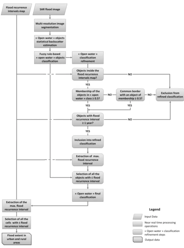
The proposed method (depicted in the flowchart in Fig. 1) provides near-real-time flood extent 122
mapping in urban and rural areas using a high-resolution SAR C-Band HH-polarized flood 123
image as input data. Horizontal polarization is preferred over vertical polarization or cross 124
polarization as it generally yields the highest contrast between open water and upland locations 125
(Brisco et al., 2008). The SAR image must be speckle-filtered (Senthilnath et al., 2013), 126
geocoded, and calibrated to obtain backscatter values. 127
RP data estimated for each point of the study area are also required. These values are 128
generally estimated using one dimensional (1D) or two-dimensional (2D) hydraulic modelling. If 129
such data is not available for the study area, an alternative method for RP estimation at each 130
point of the study area is described in section 2.1. This estimation should be carried out prior to 131
near-real-time operations. 132
7 133
Fig. 1: Flowchart of the proposed approach. 134
135
The first step in near-real-time operations is the detection of open water flooded areas on SAR 136
flood image using an approach that combines object-oriented segmentation, calibration of the 137
8 statistical distribution of “open water” objects’ mean backscatter values, and thresholding-based 138
fuzzy classification. This initial classification of “open water” objects is then refined using the 139
degree of membership of each object in the “open water” set and its maximum RP. Following 140
this classification refinement, the RP associated with the maximum extent of the refined “open 141
water” classification is extracted. Finally, floodplain points for which the RP is less than or equal 142
to this maximum RP are selected to create the final flood map. These near-real-time processing 143
steps will be described in detail in the following sections. 144
145
2.1 Method for flood return period estimation 146
147
RPs are usually computed, for some selected RPs, using a 1D or 2D hydraulic model forced by 148
statistically estimated hydrological inputs. Hydrological and hydraulic models, set up for a given 149
area, are generally not available for the public. However, their outputs in terms of RP shorelines 150
or extents are publicly released, for some selected RPs. Between 3 and 5 RP shorelines are 151
usually made available, depending on the country or region, and are widely used as risk criteria 152
for land use planning. Therefore, the RP of most points of the floodplain remain unknown. 153
Running a hydraulic simulation can be complex and time consuming. We hereby propose a 154
simple and efficient method to estimate the RP at each point of the floodplain, based on the 155
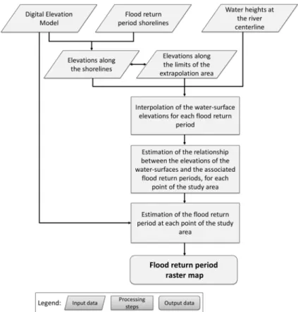
available RP shorelines in the study area and on topographic elevation data. A flowchart of this 156
method is presented in Fig. 2. 157
9 158
Fig. 2: Flowchart of the flood return period raster map estimation. 159
160
The inputs to this method are: 161
1. Available RP shorelines for the river. The positions of such shorelines along the river are 162
estimated using 1D or 2D hydraulic modelling, and they are often made available in the 163
form of polygons or polylines. A minimum of three different RP floodplain shorelines are 164
required to estimate consistent RP at each point of the floodplain. 165
2. Water height values at the river centreline associated with each RP shoreline available. 166
The water-surface elevations at the river centreline are also estimated by using either a 167
1D hydraulic model (in which case one value of water height at the river centreline 168
coincides with the values of water height of the given section) or a 2D hydraulic model 169
10 (in which case a water height value is available for each cell of the model at the river 170
centreline, including one value for each cell located along the river centreline). 171
3. A high-resolution digital elevation model (DEM) of the ground elevations in the area. In 172
order to allow extraction of accurate water levels along the RP shorelines, this DEM 173
should be the same as the one used to estimate the position of these shorelines. If this 174
DEM is not available, a DEM with identical vertical and horizontal accuracies must be 175
used. Also, the user must ensure that no major changes in ground elevations occurred 176
between the time the flood return shorelines were estimated and the time the alternative 177
DEM was produced. It should be noted that the higher the vertical and horizontal 178
accuracies of the DEM used are, the more precise the RP estimation at each point of the 179
floodplain should be. 180
181
RP estimation at each point of the floodplain follows three steps. In order to facilitate 182
understanding of this procedure, its different elements are gathered in a single figure (see Fig. 183
3), which also presents an example of RP of a point in the floodplain. 184
11 185
Fig. 3: General scheme of RP estimation at a given point in the floodplain. 186
187
First, the elevations of the water surface associated with each RP are generated, using a spatial 188
interpolation technique. This involves the creation and aggregation of the points used for the 189
generation of each water surface. To do so, each RP shoreline is converted into feature points 190
and the elevations of these points are extracted from the DEM. For each RP available, a set of 191
points is created by grouping the water height feature points at the river centreline with the 192
feature points along the RP shoreline. Then, a 150 m-buffer is created around the shorelines of 193
the highest RP available, and its outer boundaries are converted into feature points. These 194
points represent the extrapolation area limits, which allow to estimate the RP for the points of 195
the study area located outside the highest RP available. These points are added to each RP set 196
of points. By doing so, we ensure that all the RPs water surfaces will have the same number of 197
rows and columns. The elevation of each point located along the extrapolation area is estimated 198
using the k-nearest neighbour regression method (Altman, 1992), based on the elevation of the 199
100 nearest points located along the RP shoreline. Finally, each RP water surface is spatially 200
12 interpolated from its set of points, which is now composed of the river centreline points, along 201
the RP shoreline and the outer limits of the extrapolation area. The interpolation is done using a 202
natural neighbour interpolation technique (Sibson, 1981). The RPs water surfaces created are 203
raster surfaces with the same number of rows and columns, in which cell values represent the 204
water surface elevation, for a given RP. Their spatial resolution is set to be the same as the 205
spatial resolution of the DEM used. 206
Second, for each cell common to all the RP raster water surfaces previously created, the 207
relationship between water height at the cell location and the RPs associated with these water 208
heights is estimated. For instance, if 3 RPs water surfaces with the same number of rows and 209
columns have been generated, this relationship will be estimated for each cell using 3 water 210
heights and 3 RPs. This relationship is expressed by the following non-linear regression 211 function: 212 = (1) 213
where is the water surface elevation at the cell position (in metres), extracted from the water 214
surface raster, and is the RP associated with that water surface (in years). and are the 215
non-linear regression parameters to be estimated. 216
Lastly, RP is estimated for each point of the floodplain using the elevation of the cell and the 217
and parameters specific to that cell. RPs are estimated using the following equation: 218
= (2)
219
where is the elevation of the cell, extracted from the high-resolution DEM of the area, and 220
13 and are the parameters of the non-linear regression previously estimated for the cell. is the 221
RP of the cell, in years, and represents the return period at which the area represented by the 222
cell should be flooded. 223
The results are stored in a raster map, which will be designated as the “flood return period map” 224
in the following steps of the method. The spatial resolution of this raster map must be the same 225
as the spatial resolution of the DEM used. The estimated RPs are expressed per cell, in years. 226
It is worth mentioning that even if the use of an extrapolation technique is essential to estimate 227
the RP of the points located above the shoreline of the highest RP available, as well as between 228
the shorelines of the lowest and highest RP available, it also leads to less reliable RP 229
estimations. This can be considered as a limitation of this method. However, and this is an 230
important point, the RPs estimated at each point of the floodplain using this method are relative 231
values, which are not considered as representative of the water discharge needed to flood this 232
point. These values should rather be regarded as indicators of the potential RP of a cell, 233
considering its position and elevation in the floodplain with respect to the characteristics of the 234
RP shorelines available. 235
236
2.2 Segmentation of the SAR image 237
238
High-resolution SAR data enables precise detection of individual features on the earth’s surface, 239
but the use of high spatial resolution also results in significant within class backscatter variances 240
and therefore, high inter-class spectral confusion (Voigt et al., 2008; Martinis et al., 2011). This 241
makes high-resolution SAR image processing with traditional per-pixel methods challenging, 242
and the generated results may be affected by inherent speckle noise of SAR imagery (Esch et 243
14 al., 2006). If the application of speckle filters helps to reduce this effect, speckle noise remains 244
at least partially present (Senthilnath et al., 2013). An alternative to per-pixel methods is object-245
based classification. Objects are created by the sequential merging of neighbouring pixels 246
based on similarity criteria, such as their spectral characteristics, their shape, or their texture. 247
This results in non-overlapping homogeneous objects that correlate with real-world objects 248
(Blaschke et al., 2014). One of the advantages of the object-based approach is that it provides a 249
preliminary delineation of open water areas, through objects readily usable for classification 250
(Blaschke et al., 2010). 251
Segmentation of high-resolution SAR flood images into objects is performed by using the multi-252
resolution segmentation module of the eCognition Developer 8 software. This algorithm has 253
already proved successful at segmenting rural open water areas in a high-resolution TerraSAR-254
X image, in a study by Mason et al. (2012). This image segmentation algorithm is a bottom-up 255
segmentation method based on a pairwise region-merging technique (Definiens AG, 2011). 256
Segmentation begins with single-pixel objects, which are iteratively merged with neighbouring 257
pixels until the object’s growth exceeds the maximum allowed heterogeneity criterion set by the 258
user through a scale parameter. The object homogeneity criterion is defined by a combination of 259
spectral values (or colour) and shape properties, based on smoothness and compactness 260
criteria. As open water areas are generally characterized by dark tones and irregular shapes, 261
the shape criterion is set low to increase the relative contribution of spectral values in the 262
homogeneity criterion, and the compactness value is set medium to limit over-segmentation of 263
open water objects due to local variations in backscatter values. After trial-and-error 264
experimentation with the segmentation procedure, a shape value of 10% and a compactness 265
value of 50% were selected. The scale parameter was set to 5, to enable estimation of the 266
statistical distribution of “open water” on a large amount of data representatives of the class. 267
15 2.3 Statistical estimation of "open water" object backscatter
269 270
Next, the probability density function (PDF) of the mean backscatter values of the SAR image 271
objects associated with open water must be estimated. This method was successfully applied in 272
Matgen et al. (2011) and in Giustarini et al. (2013) for open water area detection on ENVISAT 273
and TerraSAR-X flood images, respectively. In these two studies, the statistical distribution of 274
“open water” backscatter values was estimated using a gamma PDF to extract the parameters 275
of a region-growing approach. The choice of a gamma PDF was based on previous work by 276
Ulaby et al. (1986), who ascertained that the PDF of homogeneous surfaces with backscatter 277
variability, which is mainly due to speckle, is of the gamma type. Alternative PDF types, such as 278
the K-distribution and the RiIG distribution functions, were tested by Giustarini et al. (2013) and 279
found not to provide more precise empirical distribution-fitting than a gamma function. 280
The gamma probability density function used for estimating the mean statistical distribution of 281
open water object backscatter can be expressed as follows: 282
( | , ) =( − )
Γ( ) . (3)
283
Where represents the backscatter value of each pixel in the SAR image, expressed in dB; 284
is the shape parameter of the gamma distribution, and is the scale parameter. As gamma 285
distribution is computable only for positive values, the backscatter values are shifted to positive 286
for the entire range of empirical values. Therefore, the parameter represents the minimum 287
backscatter value of the SAR image, in dB. 288
16 The following formula of the gamma distribution mode was used to facilitate the fitting procedure 290
(Matgen et al., 2011): When ≥ 1, 291
= ( − 1). + . (4)
292
The gamma probability density function can thus be expressed as: 293 ( | ) = . ( ) .( ) . (5) 294
Therefore, for a given value of (in dB), only the value has to be optimized to determine 295
. A local maxima estimator, which searches for the mode value with the highest probability 296
density in the lowest backscatter values, is used to automatically set a first-guess value for the 297
parameter. Then, for all plausible values close to , the parameter is iteratively optimized 298
using a non-linear least square fitting process. Note that the search interval at each iteration is 299
automatically set by the non-linear least square regression fitting process, based on the Port 300
algorithm for non-linear least squares (Fox et al., 1977). For each set of and parameter 301
values, the Root Mean Square Error (RMSE) between the theoretical density function and the 302
empirical density function is estimated. The values of the and parameters providing the 303
lowest RMSE are set as the optimum parameters for the estimation of the gamma PDF of the 304
open water object mean backscatter values. 305
If part of the open water area on the SAR flood image is affected by wind or rainfall, the 306
histogram of image objects mean backscatter values might not be bimodal. In such cases, the 307
algorithm is automatically directed towards an alternative option. The algorithm estimates the 308
first derivative of the cubic smoothing spline fitted on the experimental PDF of the mean 309
17 backscattering values of the SAR image objects. The first local positive minimum of the first 310
derivative, which represents the first point where the spline stops increasing or reaches a 311
plateau, is set as a first-guess value for the parameter. The optimal and parameters 312
are then estimated using the previously described method. However, the proposed approach is 313
not applicable if the image object’s histogram of mean backscatter values is strictly unimodal. 314
This may happen if the SAR image is dominated by water or land surfaces, if most open water 315
surfaces of the SAR image are affected by wind, or if the open water areas are small. This is a 316
limitation of this approach. 317
318
2.4 Fuzzy rule–based classification of “open water” objects 319
320
The fourth step is the classification of “open water” objects in the SAR flood image (Fig. 1). To 321
account for potential overlap of the backscatter values of open water surfaces and those of 322
other land use types, a fuzzy rule–based classification method is used (Macina et al., 2006). 323
Like traditional classification using a single threshold, fuzzy set theory eventually results in a 324
binary classification. However, one of the advantages of fuzzy set theory is that it also enables 325
estimation of the degree of membership of the elements of a fuzzy set (in this case, SAR image 326
objects) in a given class. A standard Z-shaped fuzzy membership function is used to assess the 327
SAR image object’s membership to the “open water” class (Pulvirenti et al., 2013). According to 328
this function, the lower the image object’s backscatter value, the higher its membership degree 329
to the class. The standard Z-shaped fuzzy membership function is expressed by: 330
18 ( , , ) = ⎩ ⎪ ⎪ ⎨ ⎪ ⎪ ⎧ 1, ≤ 1 − 2 − − , ≤ ≤ + 2 2 − − , + 2 ≤ ≤ 0, ≥ (6) 331
where is the mean backscatter value (in dB) of the object for which the membership degree 332
is estimated and and are the fuzzy threshold parameters of the membership function, and 333
are expressed in dB. 334
The parameters and of the fuzzy set are automatically extracted from the theoretical 335
values of the gamma probability density function fitted on the open water object mean 336
backscatter values. Parameter is set as the mode parameter of the theoretical “open water” 337
gamma distribution. This is considered the maximum backscatter value at which no overlap 338
between open water and other land use type backscatter values should happen. Parameter 339
is set as the 99th percentile of the theoretical “open water” gamma distribution (Matgen et al., 340
2011). This high percentile value may induce some over-detection, as the tail of the “open 341
water” gamma distribution may largely overlap with the backscatter values of the other land use 342
types. However, it should also enable the inclusion of open water objects whose mean 343
backscatter values are affected by protruding vegetation or small-scale anthropogenic elements. 344
This first level classification is defined as the initial classification of “open water” objects. 345
346
347
19 2.5 Refinement of “open water” object classification
349 350
Next, the classification of “open water” objects is refined in order to reduce over-detection of 351
open water areas (see Fig.1). This refinement will have no impact on the under-detections 352
resulting from the application of the fuzzy rule-based classification, as objects whose mean 353
backscatter is higher than the value of parameter are definitively excluded from “open water” 354
classification. 355
Two characteristics of the objects classified as “open water” are used for classification 356
refinement: their membership degree to the “open water” class and their RP value, extracted 357
from the flood return period map. Before proceeding with the refinements steps, objects located 358
outside the area covered by the RP map (that is, beyond the limits of the extrapolation area), 359
are automatically excluded from “open water” classification, as their location is considered too 360
far from the main river channel to be flooded. 361
The first classification refinement step uses the object’s membership degree to the “open water” 362
class. Objects whose membership degree is superior or equal to 0.5 are selected. Then, objects 363
whose membership degree is inferior to 0.5, but whose border has a connection of at least one 364
pixel with the border of an object whose degree of membership is superior or equal to 0.5, are 365
also included in the selection. Despite the low membership degree of these objects to the “open 366
water” class, the spatial connection between these objects and objects with a high degree of 367
membership in the class indicates a high probability of being actually flooded. It is worth 368
mentioning that hedgerows or wind-affected water surfaces should not be included in adjacent 369
flooded objects by this rule. Indeed, the diffuse surface scattering of wind-affected surfaces and 370
the diffuse volume scattering of hedgerows result in objects with high mean backscattering 371
values. These values should be notably higher than the value of parameter , which 372
20 determines the higher threshold of the Z-shaped fuzzy membership function used for open 373
water fuzzy logic classification. Therefore, these objects have a membership value of “0” to the 374
“open water” class and are permanently rejected from the classification. 375
The second classification refinement step uses the RP of “open water” objects. Then, the 376
maximum RP of each object selected in the previous classification refinement step is calculated 377
using the flood return period map. To limit non-water pixels from being erroneously included in 378
the objects during the multi-resolution segmentation, the 99th percentile of the RP of the object 379
is considered as the maximum RP. 380
Objects corresponding to permanent water surfaces, such as the main river channel, lakes, and 381
reservoirs may be numerous, and the very low RP of these objects is likely to influence the 382
results of the final classification refinement step. Therefore, objects for which the RP’s 99th 383
percentile is less than one year are removed from the selection. 384
Next, all the selected “open water” objects are merged together to create one single “open 385
water” object. The maximum RP of this object is extracted from the flood return period map. To 386
limit the influence of misclassified pixels on the RP estimate, the 99th percentile of the 387
maximum RP is used. 388
Finally, the objects classified as “open water” in the initial fuzzy logic classification but whose 389
RP’s 99th percentile is inferior or equal to the previously computed maximum RP are included in 390
the final “open water” refined classification. 391
392
393
21 2.6 Creation of the flood map in urban and rural areas
395 396
Flood map creation for both the urban and the rural areas relies on two reasonable 397
assumptions. The first is that classification of the “open water” areas enables detection of the 398
maximum extent of the flood. The second is that an object whose RP is less than or equal to 399
that of the maximum extent of the flood can logically be considered flooded. 400
The method used for the final flood extent mapping in urban and rural areas follows two steps. 401
First, the maximum RP of the refined “open water” classification is estimated using the flood 402
return period map. To limit the impact of non-water pixels erroneously included in the “open 403
water” objects, the 99th percentile of the RP is used again. Every cell of the flood return period 404
raster map whose RP is inferior or equal to this maximum RP are then selected. The selected 405
cells represent the maximum extent of the flood in urban and rural areas at the time of SAR 406 image acquisition. 407 408 3. Case study 409 410 3.1 Flooding event 411 412
The data used to test the proposed method were acquired during the 2011 Richelieu River 413
flood, in southern Quebec, Canada. This river flows from south to north in the Saint Lawrence 414
lowlands, an area characterized by low relief and gentle slopes. From mid-April to the end of 415
June 2011, the Richelieu River was subject to major flooding that resulted from the melt of large 416
quantities of snow accumulated during the winter and unusually heavy and continued rainfalls 417
22 between mid-April and May. The river exceeded its bankfull discharge (1064 m³/s; 27.07 m in 418
gauged level, relative to sea level, at the Rapid Fryers gauging station) on April 17th, when the 419
flow increased to 1080 m³/s (27.58 m in gauged level). Water levels continued to rise and 420
reached their peak on May 6th, with a discharge of 1550 m³/s (30.21 m in gauged level). The 421
water level began to decrease only on June 2nd, and it took three more weeks, until June 22nd, 422
for the Richelieu River to return to below bankfull. This major event resulted in the flooding of 423
numerous urban and residential areas located along the river and of large areas of rural land. 424
More than 2500 buildings were flooded, and around 1600 people were forced to evacuate their 425
homes (OSCQ, 2013). 426
The majority of the buildings in this area are one or two stories high, with basements. Some 427
industrial warehouses and shopping centers, featuring large parking lots, are located in the area 428
of interest. Streets are organized in a grid pattern, which makes this area rather representative 429
of typical medium-sized towns in Canada. 430
431
3.2 RADARSAT-2 images 432
433
Two RADARSAT-2 (C-Band) images are available to assess the performance of the proposed 434
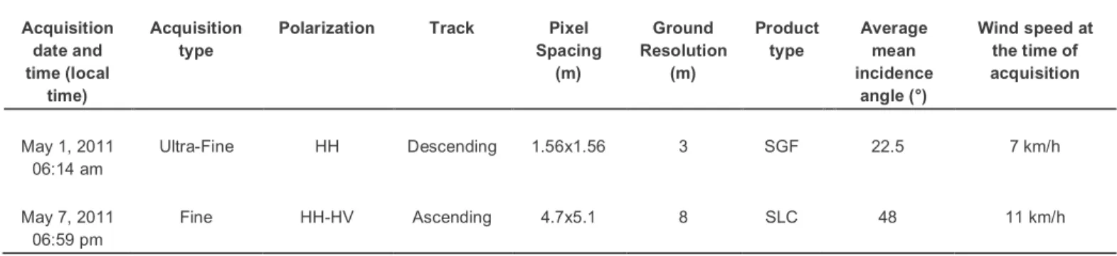
method. Their characteristics are summarized in Table 1. The first image is an Ultra-Fine Mode 435
Scene acquired on May 1, 2011 at 07:14 am local time, in HH polarization, during a descending 436
orbit pass (Fig. 4A). This image is a SAR Georeferenced Fine (SGF) product, with 1.5 x 1.5 m 437
pixel spacing (3 x 3 m after pixel resampling) and a mean incidence angle of 23°. No rainfall 438
was recorded in the 72 hours preceding the time of image acquisition, resulting in unsaturated 439
soil conditions in the non-flooded areas. Wind speed was moderate (7 km/h, blowing from east), 440
but the steep incidence angle (23°) of this SAR image makes it sensitive to Bragg resonance 441
23 effects. Bragg resonance leads to increased backscatter from open water surfaces, which can 442
be seen in Fig. 4C. 443
Table 1: Characteristics of the RADARSAT-2 flood images used to test the proposed method 444 Acquisition date and time (local time) Acquisition type
Polarization Track Pixel Spacing (m) Ground Resolution (m) Product type Average mean incidence angle (°) Wind speed at the time of acquisition May 1, 2011 06:14 am Ultra-Fine HH Descending 1.56x1.56 3 SGF 22.5 7 km/h May 7, 2011 06:59 pm Fine HH-HV Ascending 4.7x5.1 8 SLC 48 11 km/h 445
The second SAR image is a Fine Mode Scene acquired on May 7 at 06:59 pm local time, in HH-446
HV polarization, during an ascending orbit pass (Fig. 4B). Only the HH polarization was used. 447
This image is a Single Look Complex (SLC) product, with 4.7 x 5.1 m pixel spacing (8 x 8 m 448
after pixel resampling) and a mean incidence angle of 48°. Significant rainfalls (> 70 mm) were 449
recorded in the four days before image acquisition, resulting in wet soil conditions in the non-450
flooded areas. Winds were blowing at 11 km/h from northeast. 451
24 452
Fig. 4: (A) RADARSAT-2 (HH) Ultra Fine Mode image acquired on May 1, 2011. (B) 453
RADARSAT-2 (HH-HV) Fine Mode image acquired on May 7, 2011; location of the Rapid Fryers 454
gauging station indicated. Red boxes represent the areas covered by the SAR sub-images and 455
by their associated validation data. (C) Open water areas affected by wind disturbance. 456
457
To decrease the contribution of speckle, a Gamma-Map filter (Lopes et al., 1993) with a window 458
size of 5 x 5 pixels was applied. This adaptive speckle filter preserves the edges of the features, 459
which is advantageous for the object-oriented segmentation step of the proposed method. To 460
reduce processing time associated with the object-oriented segmentation of the images, 461
subsets of the RADARSAT-2 scenes were created. Each sub-image covers an area identical to 462
that covered by its associated validation data (red boxes in Fig. 4). 463
25 464
3.3 Validation dataset 465
466
Two very-high-resolution multispectral images were used to validate the flood extent maps 467
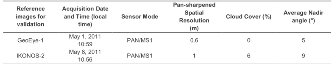
produced by the algorithm. Their characteristics are summarized in Table 2. On May 1, 2011, 468
the GeoEye-1 satellite overpassed the Richelieu River at 01:09 pm local time during clear-sky 469
conditions, providing pan-sharpened multispectral scenes of the flooded areas with a spatial 470
resolution of 0.6 m. At the time of acquisition, the water level recorded at the Rapid Fryers 471
gauging station was 27.47 m (relative to sea level), identical to the water level recorded at the 472
time of the RADARSAT-2 Ultra-Fine Mode acquisition earlier that day. The limits of the flood 473
should thus be similar in the two scenes. The mosaic of GeoEye-1 scenes covers only a small 474
part of the area imaged by the RADARSAT-2 scene (red box in Fig. 4A). Therefore, validation of 475
the final flood extent map was possible only for a 13.5 km stretch of the Richelieu River. 476
However, despite its reduced size, this section contains a wide range of flooded land cover 477
types, including built-up areas, fields, forested areas, and other vegetation. 478
Table 2: Characteristics of the very-high-resolution multispectral GeoEye-1 and IKONOS-2 pan-479
sharpened images used to validate RADARSAT-2–derived flood extent maps. 480
Reference images for validation
Acquisition Date and Time (local
time) Sensor Mode Pan-sharpened Spatial Resolution (m)
Cloud Cover (%) Average Nadir angle (°) GeoEye-1 May 1, 2011 10:59 PAN/MS1 0.6 0 5 IKONOS-2 May 8, 2011 10:56 PAN/MS1 1 6 9 481
The image used to validate the flood extent map generated from the RADARSAT-2 Fine Mode 482
image acquired on May 7, 2011 consists of a mosaic of pan-sharpened IKONOS-2 images with 483
26 1 m spatial resolution acquired on May 8, 2011 at 10:56 am local time, during almost clear sky 484
conditions (cloud cover ˂6%). Despite the delay of almost 27 hours between acquisition of the 485
RADARSAT-2 image and that of the IKONOS-2 image, the water levels measured at the Rapid 486
Fryers gauging station were very similar (27.57 m and 27.53 m, respectively). Thus, this delay 487
should not lead to important differences between the SAR-derived flood extent map and the 488
validation map. The mosaic of IKONOS-2 images covers the entire portion of the river that was 489
severely impacted by the flood, enabling us to test the algorithm on a section of the river more 490
than 29.5 km long (red box in Fig. 4B). This section contains large areas of flooded fields and 491
vegetation, and numerous flooded built-up areas. 492
Special care was paid to geocorrection of the pan-sharpened images in order to ensure their 493
precise overlap with the RADARSAT-2 flood images. For both SAR images, sub-pixel precision 494
was achieved. The flood extent was manually delineated on both pan-sharpened images (Fig. 495
5). The very high resolution of these images, minimal cloud cover presence, and linear shape of 496
the study area and of the flooded areas made delineation of the open water rather easy in most 497
locations. However, the delineation task was more complex in urban areas. It was indeed 498
particularly difficult to visually detect, and therefore to delineate, the limit of the flood around 499
each building in residential areas, because of the important presence of garden arrangements 500
and vegetation. Also, the distinction between flooded and unflooded lawns, which colours are 501
rather similar on the pan-sharpened images, was not always obvious. Therefore, decision has 502
been made to consider the buildings around which the limit of the flood could not be clearly 503
seen as flooded, as well as buildings having at least one side in contact with the flood. 504
Conversely, buildings around which the flood could easily be delineated were considered 505
unflooded. Some difficulties also arose during flood delineation inside vegetated areas located 506
along the river, such as woods and wetlands. Most of these areas were entirely flooded due to 507
their close proximity to the river channel, but small areas within them were protected from water, 508
27 due to higher ground elevations. These small areas are often partially masked by vegetation, 509
and their manual delineation was challenging. Therefore, some of them may have been 510
considered as flooded in the validation datasets. Lastly, the limit between flooded and water-511
saturated but non-flooded soils was not always obvious in certain flooded fields, and was made 512
more complex by the presence of wind. 513
28 514
Fig.5: (A) Zoom into the flood validation map obtained from manual delineation on the very-high-515
resolution IKONOS-2 image of the Richelieu River acquired on May 8, 2011; (B) Location of the 516
zoomed area on the RADARSAT-2 Fine Mode flood image acquired on May 7, 2011. 517
29 3.4 Flood return period data
518 519
The Digital Elevation Model (ground surface elevations) for the Richelieu River basin; the 2-, 20-520
and 100-year RP shorelines available for the river; and the water heights at the river centreline 521
for each RP were used to produce the flood return period map for the Richelieu River floodplain. 522
The shorelines are polyline features and the water heights at the river centreline are point 523
features, with water height values attached in a geodatabase. The three RP standards used for 524
floodplain mapping in the province of Quebec are 2, 20 and 100 years. These RP shorelines 525
were generated by the Centre d’Expertise Hydrique du Québec (CEHQ), the governmental 526
agency in charge of their production in Quebec. This data, as well as that of more than 600 527
other river stretches throughout the province, are available on demand from the CEHQ, 528
The data for the river stretch at study was updated in 2006 by the CEHQ. Data from the Rapid 529
Fryers gauging station (located in Fig. 4) was used to perform the statistical analysis necessary 530
to estimate the discharge associated with each RP (CEHQ, 2006). A Log-Pearson type III 531
distribution was adjusted on 28 annual maximum discharge values recorded at this station 532
between 1972 and 2000 (minimum of 579 m³/s and maximum of 1260 m³/s). The Chi-square 533
goodness of fit test applied to the distribution shows a p-value of 0.0576. 534
A stage-discharge relation method was used to estimate the water level associated with each 535
RP for 29 sections positioned along the river according to its geomorphological characteristics. 536
Water levels and their simultaneous discharge values were first recorded at each section during 537
several field surveys. Then, stage-discharge relations were defined for four reference sections. 538
Water levels and their simultaneous discharge values were recorded during field surveys, and 539
statistically estimated RP discharge values were used to determine the water levels associated 540
with each RP for these four reference sections. Each reference section was then used to 541
30 estimate the RP water levels of several upstream or downstream sections. This was done by 542
identifying a stage-stage relation between the water levels recorded at these sections and the 543
water levels recorded at the reference station. This stage-stage relation was used to determine 544
the water level associated with each RP for each section of the Richelieu River. Then, RP water 545
surfaces were generated using an interpolation procedure. Specifically, the HEC-GeoRAS 546
software was used to simulate the RP water surfaces, through Inverse Distance Weighting 547
spatial interpolation of the RP water levels estimated at each section. Ground elevation values 548
were then subtracted from the interpolated water surfaces, to obtain the polygons of RP 549
floodplains, from which the polylines of the floodplain shorelines were derived. These ground 550
elevation values of the area were derived from LIDAR data acquired in 2006 with a point density 551
of 1 point per metre and 0.15 m horizontal and vertical accuracy. Unfortunately, we were not 552
able to obtain information on the accuracy of these RP shorelines. 553
The DEM used in this case study to produce the flood return period map for the river stretch at 554
study is not the one used by the CEHQ for 1D hydraulic modelling. Indeed, LIDAR data 555
acquired in 2006 was limited to a narrow band exceeding the 100-year RP shoreline for a few 556
metres only. It was not appropriate for RP estimation of the points located beyond the 100-year 557
RP shoreline. Therefore, LIDAR data from April 2013, with a point density of 1 point per metre 558
and 0.15 m horizontal and vertical accuracy acquired over the entire Richelieu watershed, was 559
used to produce a DEM for the portion of the river under investigation. The spatial resolution of 560
this DEM, which represents ground surface elevations, was set to 1 m. An analysis of 561
differences in ground elevations between the 2006 and 2013 LIDAR-derived DEMs has shown 562
that these differences are limited. Therefore, the use of this data should not generate major 563
errors in the flood return period map of the Richelieu River floodplain. This map is presented in 564
Fig. 6. Note that the horizontal striations in the south-east of Fig. 6 are caused by the presence 565
31 of drainage channels which locally decrease the elevation of the ground and therefore change 566
the RP of the cells. 567
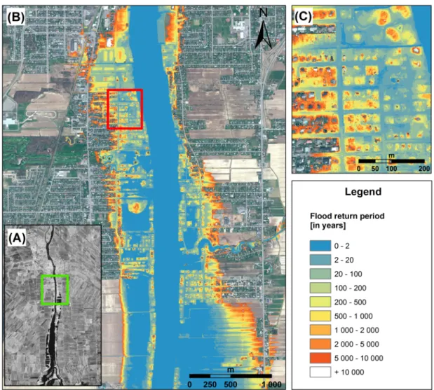
568
Fig. 6: (A) Location (green rectangle) on the RADARSAT-2 Fine Mode flood image acquired on 569
May 7, 2011 of the area of interest (red rectangle in panel (B)); (B) Flood return period map of 570
the Richelieu River superimposed on the IKONOS-2 reference image from May 8, 2011 571
(southern part of the city of Saint-Jean-sur-Richelieu depicted). The red rectangle indicates the 572
location of the zoomed area presented in panel (C); (C) Details of the RPs in a section of the 573
urban area. 574
32
4. Results
576 577
4.1 Detection of open water areas 578
579
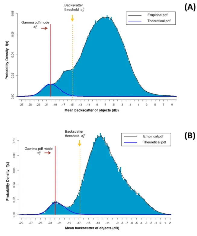
Figure 7 displays the optimized gamma PDFs fitted to the empirical image histograms of the 580
RADARSAT-2 Ultra-Fine Mode (Fig. 7A), and RADARSAT-2 Fine Mode (Fig. 7B) image 581
objects, together with the fuzzy thresholds and used for the classification of “open water” 582
objects. Table 3 reports the estimated values and standard errors of the parameter and the 583
fuzzy thresholds and for the optimized gamma PDFs for the Ultra-Fine and Fine Mode 584
flood images. 585
The contingency matrices corresponding to the accuracy of the “open water” classification steps 586
are reported in Table 4. The values in the matrices were computed by comparing the number of 587
pixels identified as open water on the optical high-resolution–derived validation maps against 588
the number of pixels contained in the “open water” objects classified by the image processing 589
algorithm. The contingency maps resulting from the final “open water” refined classification are 590
presented in Fig. 8. To enable precise visualization of the classification results, zooms into 591
areas containing under- and over-detection errors are provided. 592
Table 3: Estimated values and standard errors for the parameters and fuzzy thresholds 593
and for the optimized gamma PDFs for the RADARSAT-2 Ultra-Fine Mode and Fine Mode 594
flood images. 595
RADARSAT-2 Ultra-Fine Mode RADARSAT-2 Fine Mode
Estimated Value Standard Error Estimated Value Standard Error
0.010 0.008 0.048 0.007
-20.03 dB 0.057 -21.70 dB 0.012
33 596
597
Fig. 7: Optimized gamma PDF superimposed on the empirical image histograms of the 598
RADARSAT-2 Ultra-Fine Mode (panel A) and RADARSAT-2 Fine Mode (panel B) image 599
objects. The fuzzy thresholds and used for the classification of “open water” objects are 600
also shown. 601
34 Table 4: Quantitative evaluations of RADARSAT-2–derived “open water” detections
602 Open water classification steps % correctly classified* % under detection* % over detection* RADARSAT-2 Ultra-Fine Mode Initial classification 65 35 30 Refinement using membership degree 64 36 18 Refinement using RP 64 36 1 RADARSAT-2 Fine Mode Initial classification 88 12 10 Refinement using membership degree 87 13 5 Refinement using RP 87 13 2
* % of pixels identified as open water on the validation data sets
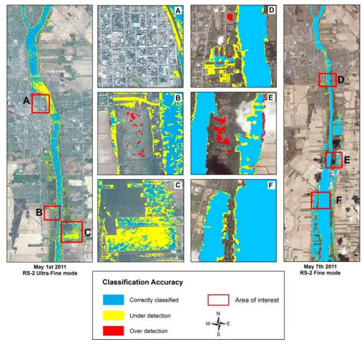
35 604
Fig. 8: Contingency maps of the final refined classification of “open water” objects deriving from 605
the application of the method to the RADARSAT-2 Ultra-Fine and Fine Mode flood images. 606
607
4.1.1 Analysis of “open water” under-detection 608
From Table 4, it can be observed that the ability of the fuzzy thresholds and to correctly 609
classify “open water” objects varies between the two SAR images. While 88% of the flooded 610
pixels were correctly identified on the Fine Mode flood image using these fuzzy thresholds, only 611
36 65% of the flooded pixels were accurately identified on the Ultra-Fine Mode flood image. The 612
high rate of "open water" under-detection in the Ultra-Fine Mode case study can be explained 613
by the significant presence of waves and ripples on the open water surfaces. This produced an 614
important increase in backscatter values of the “open water” areas and a substantial overlap 615
between mean backscatter values of “open water” and other land-use types. This overlap is 616
particularly obvious when looking at the empirical histogram of the mean backscatter of the 617
objects in the SAR image, displayed in Fig. 7A. 618
The 12% under-detection associated with the RADARSAT-2 Fine Mode “open water” object 619
classification occurred mainly along the borders of inundated fields in rural areas, and along the 620
edges of the main river channel and small tributary rivers (panels D to F in Fig. 8). The 621
difference in spatial resolution between the Fine Mode image and the IKONOS-2 image (the 622
source of the validation data) partly explains this under-detection. However, it is also imputable 623
to the presence of vegetation along the edges of open fields and the river, which tends to 624
increase the SAR signal return due to double-bounce scattering between the soil and the 625
vegetation layers. This effect is also responsible for part of the under-detection on the Ultra-Fine 626
Mode flood image (see panels B and C in Fig. 8). Thus, not all of the under-detection errors are 627
imputable to the image processing algorithm; some result from the inherent limitations of the 628
SAR C-Band imaging technique. 629
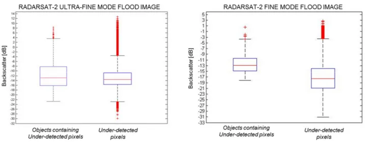
According to Matgen et al. (2011), backscatter values between -24 dB and -10 dB can be 630
considered appropriate for open water pixels for most currently available sensors. Analysis of 631
the backscatter values of the under-detected “open water” pixels in the two case studies shows 632
that many pixels with backscatter values typical of open water were excluded from the “open 633
water” classification because they belonged to objects with mean backscatter values that were 634
higher than the fuzzy membership degree defined for open water (see Fig. 9). Thus, in spite of 635
the attention that was paid to the selection of optimal parameter values for the multi-resolution 636
37 segmentation procedure, image segmentation inaccuracies remained locally present. However, 637
the impact of these inaccuracies on the classification results was moderate, as they were 638
responsible for only 4% and 0.4% of the under-detections on the Ultra-Fine Mode and Fine 639
Mode images, respectively. 640
641
Fig. 9: Boxplot of the mean backscatter values of objects containing under-detected “open 642
water” pixels, and the backscatter values of under-detected pixels, for the Ultra-Fine Mode and 643
Fine Mode flood images. 644
645
4.1.2 Analysis of “open water” over-detection 646
Most of the over-detections in the initial “open water” classification on the Ultra-Fine Mode 647
image were located in urban areas, on unflooded surfaces characterized by specular-like 648
reflection, such as roads parallel to the orbit track and parking lots; areas affected by the 649
shadow effect were also a source of over-detections. Conversely, on the Fine Mode image, 650
which did not have sufficient spatial resolution to detect such fine-scale urban elements, the 651
over-detections were located in rural areas, on bare, smooth fields. These errors can be 652
38 explained by the high soil moisture at the time the image was acquired, which resulted in low 653
backscatter values from bare soils (Ulaby et al., 1986). 654
In both case studies, the benefit of using both the objects’ membership degree in the “open 655
water” class and the RP data to refine the "open water" classification is obvious, with large 656
decreases produced in the rates of “open water” over-detection (see Table 4). Classification 657
refinement based solely on the membership degree of objects enables a significant reduction in 658
over-detections, but at rates that cannot guarantee extraction of an accurate RP for flood extent 659
mapping in urban and rural areas. Classification refinement based on the classified objects’ RP 660
is thus also essential. For information purposes, the RPs used for “open water” classification are 661
of 609 years in the Ultra-Fine mode case study and of 540 years in the Fine mode case study. 662
As shown in Table 4, the over-detections of “open water” areas were reduced to 2% for the Fine 663
Mode image and to 1% for the Ultra-Fine Mode image. In both case studies, the decrease in 664
classification accuracy associated with the classification refinement was only 1%. Therefore, 665
and as presumed in section 2.5, the use of the objects’ membership value and their spatial 666
connection to objects with a high membership degree in the “open water” class does not result 667
in the inclusion of objects containing hedgerows or wind-affected water surfaces in the “open 668
water” class. This tends to validate the “superior or equal to 0.5” membership degree rule and 669
the use of RPs for refining the “open water” classification. 670
After these two classification refinement steps, most of the remaining over-detection is located 671
at the upper boundaries of the flooded fields and in vegetated flooded areas (see panels B, E, 672
and F in Fig. 8). Over-detection at the upper boundaries of the flooded fields was more 673
important in the Fine Mode image case study than in the Ultra-Fine Mode case study. Again, 674
this can be related to the difference between the spatial resolution of the Fine Mode image and 675
the IKONOS-2 scene used as evidence of the flooding extent. An additional factor is that the 676
flood was receding by the time these images were acquired, and visually distinguishing between 677
39 the water-saturated soils and the flooded soils was locally laborious at the extremities of open 678
water areas. This may have led to local inaccuracies in the IKONOS-2–derived validation flood 679
map. 680
The remaining over-detections due to specular backscatter from unflooded areas (parking lots, 681
shadow areas around buildings, etc.) were trivial in both case studies. Only one non-flooded 682
parking lot located beside the river was classified as "open water" on the Fine Mode flood image 683
(see Fig. 8D), while no error of this type is to be found on the Ultra-Fine Mode image (see Fig. 684
8A). These results demonstrate the very good capacity of the proposed method to deal with 685
such areas, which are considered a significant impediment to precise flood detection in urban 686
areas using high-resolution SAR imagery. 687
Most of the under-detections were caused by the presence of wind on water surfaces or by 688
double bounces from vegetation. Thus, modification of the fuzzy threshold toward higher 689
backscatter values would not result in a significant reduction of under-detections and would 690
come at the cost of increased over-detections of “open water” areas. Conversely, modification of 691
the fuzzy threshold towards a lower percentile of the gamma distributions would reduce over-692
detection, but it would also result in increased under-detections of open water areas. 693
694
4.2 Accuracy of flood mapping in urban and rural areas 695
696
The maximum RP extracted from the “open water” classification was 186 years for the 697
RADARSAT-2 Ultra-Fine Mode flood image and 219 years for the RADARSAT-2 Fine Mode 698
flood image. These RPs are not and should not be considered representative of the actual RP 699
corresponding to the discharges or to the water levels registered at the gauging station at the 700
time of the SAR image acquisitions. They should rather be considered indicators related to the 701
40 maximum extent of the flooded areas identified with certainty, enabling identification of the 702
flooding status of the floodplain cells with inferior or equal RP values. 703
For each case study, the accuracy of the flood extent map that resulted from application of the 704
extracted RP across the entire floodplain is reported in the contingency matrices shown in Table 705
5. The values of the contingency matrices were computed by comparing the number of pixels 706
identified as flooded on the validation maps to the number of pixels classified as flooded in the 707
flood extent maps. The results are considered separately for urban and rural areas, which were 708
distinguished using 1:20 000 scale land cover data provided by the Canadian National 709
Topographic Data Base (NRC, 2015). To enable qualitative evaluation of the method's 710
performance, the results are displayed as contingency maps in Fig. 10. 711
Table 5: Quantitative evaluation of the RADARSAT-2–derived flood extent maps in urban and 712
rural areas 713
Area types % correctly
classified* % under-detection* % over- detection* RADARSAT-2 Ultra-Fine Mode Urban flooded areas 86 14 13 Rural flooded areas 97 3 35 RADARSAT-2 Fine Mode Urban flooded areas 87 13 14 Rural flooded areas 98 2 3
* % of pixels identified as flooded on the validation data sets
41 715
Fig. 10: Contingency maps of the final flood extent maps in urban and rural areas. The left-hand 716
panel shows the contingency map for the May 1, 2011, case study superimposed on the 717
GeoEye-1 image, with zooms into areas of interest shown in panels A, B, and C. The right-hand 718
panel shows the contingency map for the May 7, 2011, case study superimposed on the 719
IKONOS-2 image, with zooms into areas of interest shown in panels D, E, and F. 720
From Table 5, it can be seen that 86% and 97% of the flooded pixels were correctly identified in 721
the urban and rural areas, respectively, in the May 1, 2011, case study. The extraction of a RP 722
allowing urban and rural flooded areas to be precisely mapped was unlikely, as the rate of 723
correctly detected open water flooded areas was low on the Ultra-Fine Mode image. However, 724
the combination of accurate detection of most “open water” objects located at the outer 725
42 boundaries of open water flooded areas (Fig. 8) and a low rate of open water over-estimations 726
enabled extraction of an accurate RP. The associated over-detection was 13% in urban areas 727
and 35% in rural areas. The causes of this high rate of over-detection will be analyzed in detail 728
in a following section. The results obtained in the May 7, 2011, case study were almost 729
identical, although the “open water” objects classification was significantly better: 87% of the 730
urban flooded pixels and 97% of the rural flooded pixels were correctly identified by the 731
algorithm. The associated over-detection was 14% in the urban areas and 3% in the rural areas. 732
This first overview of the flood extent mapping results suggests that accurate classification of all 733
“open water” objects on a SAR flood image is not strictly required to extract RP values precise 734
enough for flood extent mapping needs. SAR flood images that include water surfaces 735
roughened by wind can thus be used as inputs to this method. 736
737
4.2.1 Analysis of under-estimations of flooding extent 738
From Fig. 10C, one can see that two flooded residential areas (labelled U1 and U2) located by 739
the riverside were classified as unflooded by the algorithm in the two case studies. The analysis 740
of the RP of the cells located in these two areas revealed values two to eight times higher 741
(between 2,000 years and 16,000 years) than the RP used for flood extent mapping in the two 742
case studies. These over-estimations of the RP had two sources. First, due to the very similar 743
elevations of the 20-year and 100-year floodplain limits in these areas, the differences between 744
the 20-year and 100-year RP water surface elevations were very low. Therefore, small 745
variations in ground surface elevation resulted in very large increases in RP, as shown in Fig. 746
11A. Also, it can be seen that the 20-year RP water surface has higher local elevations than the 747
100-year RP water surface, which results in important inaccuracies in the RP estimates (Fig. 748
11A). This error is due to the fact that the elevation points along the 100-year RP shoreline used 749
for interpolation of the associated water surface were less numerous and were unequally 750