Bootstrap for panel data models with an application
to the evaluation of public policies
par
Bertrand G. B. Hounkannounon
Département de sciences économiques Faculté des arts et des sciences
Thèse présentée à la Faculté arts et des sciences en vue de l’obtention du grade de
Philosophiae Doctor (Ph.D.) en sciences économiques
Août 2011
Faculté des arts et des sciences
Cette thèse intitulée :
Bootstrap for panel data models with an application
to the evaluation of public policies
présentée par
Bertrand G. B. Hounkannounon
a été évaluée par un jury composé des personnes suivantes : ...Marine Carrasco... président-rapporteur ...Benoit Perron... directeur de recherche ...Silvia Gonçalves... membre du jury ...Nikolay Gospodinov... examinateur externe ...Martin Bilodeau... représentant du doyen de la FAS
Résumé
Le but de cette thèse est d’étendre la théorie du bootstrap aux modèles de données de panel. Les données de panel s’obtiennent en observant plusieurs unités statistiques sur plusieurs périodes de temps. Leur double dimension individuelle et temporelle permet de contrôler l’hétérogénéité non observable entre individus et entre les périodes de temps et donc de faire des études plus riches que les séries chronologiques ou les données en coupe instantanée. L’avantage du bootstrap est de permettre d’obtenir une inférence plus précise que celle avec la théorie asymptotique classique ou une inférence impossible en cas de paramètre de nuisance. La méthode consiste à tirer des échantillons aléatoires qui ressemblent le plus possible à l’échantillon d’analyse. L’objet statitstique d’intérêt est estimé sur chacun de ses échantillons aléatoires et on utilise l’ensemble des valeurs estimées pour faire de l’inférence. Il existe dans la littérature certaines application du bootstrap aux données de panels sans justi…cation théorique rigoureuse ou sous de fortes hypothèses. Cette thèse propose une méthode de bootstrap plus appropriée aux données de panels. Les trois chapitres analysent sa validité et son application.
Le premier chapitre postule un modèle simple avec un seul paramètre et s’attaque aux propriétés théoriques de l’estimateur de la moyenne. Nous montrons que le double rééchantillonnage que nous proposons et qui tient compte à la fois de la dimension individuelle et la dimension temporelle est valide avec ces modèles. Le rééchantillonnage seulement dans la dimension individuelle n’est pas valide en présence d’hétérogénéité temporelle. Le ré-échantillonnage dans la dimension temporelle n’est pas valide en présence d’hétérogénéité individuelle.
linéaire. Trois types de régresseurs sont considérés : les caractéristiques indi-viduelles, les caractéristiques temporelles et les régresseurs qui évoluent dans le temps et par individu. En utilisant un modèle à erreurs composées doubles, l’estimateur des moindres carrés ordinaires et la méthode de bootstrap des résidus, on montre que le rééchantillonnage dans la seule dimension indivi-duelle est valide pour l’inférence sur les coe¢ cients associés aux régresseurs qui changent uniquement par individu. Le rééchantillonnage dans la dimen-sion temporelle est valide seulement pour le sous vecteur des paramètres associés aux régresseurs qui évoluent uniquement dans le temps. Le double rééchantillonnage est quand à lui est valide pour faire de l’inférence pour tout le vecteur des paramètres.
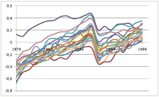
Le troisième chapitre re-examine l’exercice de l’estimateur de di¤érence en di¤érence de Bertrand, Du‡o et Mullainathan (2004). Cet estimateur est couramment utilisé dans la littérature pour évaluer l’impact de certaines poli-tiques publiques. L’exercice empirique utilise des données de panel provenant du Current Population Survey sur le salaire des femmes dans les 50 états des Etats-Unis d’Amérique de 1979 à 1999. Des variables de pseudo-interventions publiques au niveau des états sont générées et on s’attend à ce que les tests arrivent à la conclusion qu’il n’y a pas d’e¤et de ces politiques placebos sur le salaire des femmes. Bertrand, Du‡o et Mullainathan (2004) montre que la non-prise en compte de l’hétérogénéité et de la dépendance temporelle en-traîne d’importantes distorsions de niveau de test lorsqu’on évalue l’impact de politiques publiques en utilisant des données de panel. Une des solutions préconisées est d’utiliser la méthode de bootstrap. La méthode de double ré-échantillonnage développée dans cette thèse permet de corriger le problème de niveau de test et donc d’évaluer correctement l’impact des politiques pu-bliques.
Mots clés : Modèles de données de panel, Bootstrap, Evaluation de Politiques Publiques.
Abstract
The purpose of this thesis is to develop bootstrap methods for panel data models and to prove their validity. Panel data refers to data sets where ob-servations on individual units (such as households, …rms or countries) are available over several time periods. The availability of two dimensions (cross section and time series) allows for the identi…cation of e¤ects that could not be accounted for otherwise. In this thesis, we explore the use of the bootstrap to obtain estimates of the distribution of statistics that are more accurate than the usual asymptotic theory. The method consists in drawing many ran-dom samples that resembles the sample as much as possible and estimating the distribution of the object of interest over these random samples. It has been shown, both theoretically and in simulations, that in many instances, this approach improves on asymptotic approximations. In other words, the resulting tests have a rejection rate close to the nominal size under the null hypothesis and the resulting con…dence intervals have a probability of inclu-ding the true value of the parameter that is close to the desired level.
In the literature, there are many applications of the bootstrap with panel data, but these methods are carried out without rigorous theoretical justi…-cation. This thesis suggests a bootstrap method that is suited to panel data (which we call double resampling), analyzes its validity, and implements it in the analysis of treatment e¤ects. The aim is to provide a method that will provide reliable inference without having to make strong assumptions on the underlying data-generating process.
The …rst chapter considers a model with a single parameter (the overall expectation) with the sample mean as estimator. We show that our double resampling is valid for panel data models with some cross section and/or
temporal heterogeneity. The assumptions made include one-way and two-way error component models as well as factor models that have become popular with large panels. On the other hand, alternative methods such as bootstrapping cross-sections or blocks in the time dimensions are only valid under some of these models.
The second chapter extends the previous one to the panel linear regres-sion model. Three kinds of regressors are considered : individual characte-ristics, temporal characteristics and regressors varying across periods and cross-sectional units. We show that our double resampling is valid for in-ference about all the coe¢ cients in the model estimated by ordinary least squares under general types of time-series and cross-sectional dependence. Again, we show that other bootstrap methods are only valid under more restrictive conditions.
Finally, the third chapter re-examines the analysis of di¤erences-in-di¤erences estimators by Bertrand, Du‡o and Mullainathan (2004). Their empirical ap-plication uses panel data from the Current Population Survey on wages of women in the 50 states. Placebo laws are generated at the state level, and the authors measure their impact on wages. By construction, no impact should be found. Bertrand, Du‡o and Mullainathan (2004) show that neglected he-terogeneity and temporal correlation lead to spurious …ndings of an e¤ect of the Placebo laws. The double resampling method developed in this thesis corrects these size distortions very well and gives more reliable evaluation of public policies.
Résumé . . . i
Abstract . . . iv
Liste des …gures . . . viii
Dédicace . . . ix
Remerciements . . . x
Introduction Générale 1 1 Double resampling bootstrap for the mean of a panel 5 1.1 Introduction . . . 7
1.2 Panel Data Models and Assumptions . . . 8
1.3 Asymptotic Theory . . . 14
1.4 Resampling Methods . . . 17
1.5 Bootstrap Validity . . . 22
1.6 Bootstrap Con…dence Interval . . . 29
1.7 Simulations . . . 33
1.8 Conclusion . . . 35
2 Bootstrap for panel regression models with random e¤ects 57 2.1 Introduction . . . 59
2.2 Panel Data Models . . . 61 vi
2.3 Bootstrap Methods . . . 67
2.4 Theoretical Results . . . 73
2.5 Simulations . . . 78
2.6 Conclusion . . . 83
3 Bootstrapping di¤erences-in-di¤erences estimator 94 3.1 Introduction . . . 96
3.2 Di¤erences-in-di¤erences Estimation . . . 97
3.3 Bootstrap Method . . . 99
3.3.1 Residual-based Bootstrap . . . 99
3.3.2 Pair bootstrap . . . 100
3.3.3 Bootstrap Con…dence Intervals . . . 101
3.3.4 Panel Resampling Methods . . . 101
3.4 Empirical Application . . . 106 3.4.1 Speci…cation . . . 106 3.4.2 Placebo Laws . . . 108 3.4.3 Simulation Results . . . 109 3.5 Conclusion . . . 111 Conclusion Générale 113 Bibliographie 115
3.1 Time Evolution of Wage by State . . . 108
Remerciements
Je tiens à rendre hommage à mon directeur de recherche Benoit Perron pour sa disponibilité, sa patience, sa contribution à la réalisation de ce travail. Je remercie les professeurs Silvia Gonçalves et Marine Carrasco pour les discussions et les commentaires constructifs.
Mes remerciements vont aussi au Département de sciences économiques de l’Université de Montréal et au Centre Interuniversitaire de Recherche en Economie Quantitative (CIREQ) pour le soutien …nancier et la bonne am-biance de recherche.
Un remerciement tout spécial à ma famille et mes ami(e)s pour l’encoura-gement et le soutien moral. Que tous ceux qui de près ou de loin ont contribué à ce travail, reçoivent l’expression de ma sincère gratitude.
Introduction générale
Les données de panel s’obtiennent en observant plusieurs unités statis-tiques sur plusieurs périodes de temps. Leur double dimension individuelle et temporelle permet de contrôler l’hétérogénéité non observable entre in-dividus et entre les périodes de temps. Ceci permet de faire des analyses di¢ cilement faisables avec juste des séries temporelles ou des coupes trans-versales de données. L’inférence avec les modèles de panel, comme dans tout autre modèle statistique nécessite le recours à des statistiques de test. En pratique, la véritable distribution de probabilité d’une statistique de test est rarement connue. En général, nous utilisons la loi asymptotique comme ap-proximation de la vraie loi. Si la taille de l’échantillon n’est pas assez grande, le comportement asymptotique de la statistique pourrait être une mauvaise approximation de la réalité.
Un avantage important de la technique de rééchantillonnage bootstrap est de permettre d’obtenir une approximation de la distribution d’une statis-tique de test plus précise que l’approximation asymptostatis-tique lorsque la taille de l’échantillon est faible. Cette technique a été proposée originalement pour l’analyse statistique des observations indépendantes et identiquement distri-buées. Des extensions ont été faites pour l’adapter à l’analyse de données avec de la dépendance entre les observations comme les séries temporelles. La littérature sur l’utilisation du bootstrap avec des données de panel est assez restreinte. On note des exemples d’utilisation sans justi…cations théo-riques ou quand ces justi…cations existent c’est pour des cas très particuliers. Comme contribution récente à la littérature théorique, nous pouvons citer Kapetanios (2008) et Gonçalves (2010).
La double dimension des modèles de panels pose néanmoins quelques dé…s en pratique : les théories asymptotiques multiples. La façon dont on suppose
que le nombre d’unités statistiques (N) et/ou le nombre de périodes tem-porelles (T) tend vers l’in…ni, n’est pas sans consequence sur la distribution asymptotique obtenue. En pratique, face à un échantillon particulier, il n’y a pas de méthode pour choisir laquelle des distributions il faut utiliser. Le re-cours à une méthodologie qui ne di¤ère pas d’une distribution asymptotique à l’autre permettrait de contourner ce genre de problème.
L’évaluation de politiques publiques amène à considerer deux groupes d’individus : ceux qui sont par a¤ectés par la politique (groupe de traitement) et ceux qui ne sont pas a¤ectés (groupe de contrôle). Le second groupe sert de groupe de témoins et permet de contrôler des e¤ets temporels qui seraient produits en l’absence de la politique et permet d’apprécier à sa juste valeur, l’impact de de la politique publique (ou traitement). Dans l’approche la plus simpliste, on considère deux périodes de temps : une période avant la mise en place de la politique et une période après la mise en place. L’impact de la poli-tique est mésuré en prenant la variation de la variable cible dans le groupe de traitement auquel on soustrait la variation dans le groupe de contrôle. Cette technique s’appelle la methode des di¤érencesen di¤érences (ou méthode des doubles di¤érences). Elle serait tout à fait justi…ée si les individus étaient a¤ectés arbitrairement dans chacun des groupes. En réalité, la mise en place d’une intervention du pouvoir publique est justi…ée par des besoins d’objectif à atteindre. Une localité va béni…cier d’un projet particulier parce qu’on veut y réduire par exemple le taux de décrochage scolaire qui y est plus élevé que dans d’autres zone scolaires. Le choix des individus du groupe de contrôle et ceux qui sont dans le groupe de traitement est donc loin d’être arbitraire. L’appréciation du gain de la politique peut donc être est biaisé par un e¤et de sélection. Pour tenir compte du fait que l’appartenance à l’un des deux groupes peut dépendre des caractéristiques individuelles, il faut les inclure
dans l’évaluation d’impact. L’approche générale est de postuler un modèle linéaire ou la variable d’intérêt y est fonction des caractériques individuelles et d’une variable indicatrice qui prend la valeur 1 quand l’individu est af-fectée par la politique en second période et la valeur 0 sinon. Le coe¢ cient associé à cette variable indictarice mesure l’impact de la politique étudiée.
Dans une approche plus générale, on considère les deux mêmes groupes mais cette fois-ci, pendant plusieurs périodes de temps. Cette approche per-met de mieux tenir compte de la dynamique temporelle et on à ce moment des données de panel. Une di¢ culté pratique dans l’évaluation des politiques publiques est la limitation du nombre d’observation. En e¤et, avant la mise en place à une plus grande échelle, une politique peut d’abord est testée sur un échantillon, le nombre d’unités statistiques impliquées est alors modéré. La nécessité d’avoir les premiers résultats d’un programme dans un laps de temps raisonnable limite le nombre de périodes de notre panel. Cette double restriction fragilise la qualité de l’inférence que l’on a recours à l’asympto-tique. Malgré ces di¢ cultés, le chercheur doit faire de son mieux pour tirer la meilleure information de l’échantillon dont il dispose. L’utilisation des mé-thodes de bootstrap peut accroître la qualité de l’inférence.
La présente thèse examine le développement de méthodes bootstrap ap-propriés aux modèles de panel, leurs justi…cations théoriques et applications. Le premier chapitre postule un modèle simple avec un seul paramètre et s’attaque aux propriétés théoriques de l’estimateur de la moyenne1.
Le deuxième chapitre étend le précédent au modèle panel de régression linéaire. Trois types de régresseurs sont considérés : les caractéristiques indi-viduelles, les caractéristiques temporelles et les régresseurs qui évoluent dans 1Il est commun de démontrer la validité d’une méthode de rééchantillonnage pour la
le temps et par individu. En utilisant un modèle à erreurs composées doubles, l’estimateur des moindres carrés ordinaires et la méthode de bootstrap des résidus, on montre que le rééchantillonnage dans la seule dimension indivi-duelle est valide pour l’inférence sur les coe¢ cients associés aux régresseurs qui changent uniquement par individu. Le rééchantillonnage dans la dimen-sion temporelle est valide seulement pour le sous vecteur des paramètres associé aux régresseurs qui évoluent uniquement dans le temps. Le double rééchantillonnage est quand à lui est valide pour faire de l’inférence pour tout le vecteur des paramètres.
Le troisième chapitre re-examine l’exercice de l’estimateur des doubles di¤érences de Bertrand, Du‡o et Mullainathan (2004). L’exercice empirique utilise des données de panel provenant du Current Population Survey sur le salaire des femmes dans les 50 états des Etats-Unis d’Amérique de 1979 à 1999. Des variables de pseudo-interventions publiques au niveau des états sont générées et on s’attend à ce que les tests arrivent à la conclusion qu’il n’y a pas d’e¤et de ces politiques placebos sur le salaire des femmes. Ber-trand, Du‡o et Mullainathan (2004) montre que la non-prise en compte de la dépendance temporelle entraîne d’importantes distorsions de niveau de test lorsqu’on évalue l’impact de politiques publiques en utilisant des données de panel. La méthode de double rééchantillonnage développée dans cette thèse permet de corriger le problème de niveau de test et donc d’évaluer correcte-ment l’impact des politiques publiques.
Double resampling bootstrap
for the mean of a panel
Abstract
This paper considers bootstrap methods for the sample mean in panel data. It is shown that double resampling that combines cross-sectional and temporal resampling is valid under general conditions on cross-sectional and temporal heterogeneity as well as cross-sectional dependence. On the other hand, resampling only in the cross section dimension is not valid in the pre-sence of temporal heterogeneity, while block resampling only in the time series dimension is not valid in the presence of cross section heterogeneity. The bootstrap does not require the researcher to choose one of several asymp-totic approximations available for panel models. Simulations con…rm these theoretical results.
JEL Classi…cation : C15, C23.
1.1
Introduction
This paper analyzes properties of bootstrap methods in carrying out in-ference on the mean of panel data. The goal is to try to construct con…-dence intervals and conduct hypothesis tests without having to make strong assumptions regarding either the serial correlation or cross-sectional depen-dence of the data.
While there is an abundant literature on asymptotic theory for panel data models, there is much less on the bootstrap. There are some simula-tion results suggesting that some resampling methods work well in practice but theoretical results are rather limited or require strong assumptions. For example, Kapetanios (2008) recently presented theoretical results in a linear panel regression model when the cross-sectional dimension goes to in…nity, under the assumption that cross-sectional vectors of regressors and errors terms are i.i.d.. This assumption is quite restrictive and does not allow time-varying regressors or temporal aggregate shocks in errors terms. Gonçalves (2010) explores the moving blocks bootstrap in a linear regression model as well, and Palm, Smeekes and Urbain (2011) develop the bootstrap for nonstationary panel models.
Asymptotic analysis in panel models is complicated by the fact we have cross-sectional and time series dimensions. Thus, several asymptotic approxi-mations can be developed, depending on the assumptions one is willing to make on the size of these two dimensions. Typically, the resulting approxi-mations will be di¤erent, forcing an applied researcher to choose among these various approximations in order to obtain a critical value for a hypothesis test. One of the main advantages of the bootstrap in the context of panel models is that it is not necessary to make such a choice. The bootstrap will
provide valid critical values for various asymptotic scenarios under appro-priate conditions.
The paper is organized as follows. In the second section, di¤erent panel data models are presented. Section 3 presents the asymptotic theory. Sec-tion 4 presents three bootstrap resampling methods for panel data. The …fth section presents theoretical results, analyzing the validity of each resampling method. The seventh section bootstrap con…dence interval and analyzes their validity. In section 7, simulation results are presented and con…rm the theo-retical results. The eighth section concludes. Proofs of propositions are given in the appendix.
1.2
Panel Data Models and Assumptions
We suppose that we observe panel data yit for cross-sectional unit i at
time t: There are N cross-sectional units (typically households, …rms or coun-tries) and T time periods. One could consider unbalanced panels where the number of observations for each unit would di¤er, but for simplicity, we do not consider this case.
In this chapter, we consider a panel model without regressors.
yit = + it (2.1 )
where is an unknown parameter of interest and it is random. The
goal is to carry out inference on the parameter using the sample mean as estimator (which is the OLS estimator) without making strong assumptions on it. Chapter 2 will consider the more general case where regressors varying
over i and t will be included in the model. It is common to …rst analyze the properties of a bootstrap method for the sample mean before investigating
more complicated statistics.
It will prove convenient to represent our panel data as a matrix. We will do so by putting into rows the observations for each cross-sectional unit and then stacking these rows. The resulting matrix, which we denote by Y , is of dimension N T : Y (N;T ) = 0 B B B B B B B B @ y11 y12 ::: ::: y1T y21 y22 ::: ::: y2T ::: ::: ::: ::: ::: ::: ::: ::: :: ::: yN 1 yN 2 :: ::: yN T 1 C C C C C C C C A
We will analyze the properties of bootstrap methods in (2 :1 ) that do not require making strong assumptions during implementation. We will do so under various scenarios on the properties of vit: We conjecture that our
results will extend to even more general structures, and this will be the subject of future research.
We decompose it into four components :
it = i+ ft+ iFt+ "it: (2.2 )
It is customary to call i the individual e¤ect and ftthe time e¤ect. The
term iFt represents the contribution from a factor model. In that model,
each unit i is allowed to respond heterogeneously to a set of common factors Ft:Finally, the last term is the remainder and will be called the idiosyncratic
component.
Assumption A (individual e¤ects)
distribution with mean 0 and variance 2 (where 0 < 2 <
1:) and is independent of the cross-sectional and/or temporal heterogeneity.
Assumption A requires the individual heterogeneities to be independent and identically distributed with …nite variance. The assumption of a zero mean is an identi…cation assumption as any non-zero mean could be sub-sumed into the overall mean : The i.i.d. assumption, strong for classical asymptotic distribution is however important for bootstrap validity because i.i.d. bootstrap will be used in the cross-sectional dimension.
Assumption B (time e¤ects)
fftg is a stationary and -mixing process with mixing coe¢ cients (j);
E (ft) = 0 and fftg veri…es Ibragimov’s assumptions, that is 9 2 (0; 1)
such that E jftj2+ < 1 and 1
X
j=1
(j) =(2+ ) < 1 with …nite long-run
va-riance V1 f = 1 X h= 1 Cov (ft; ft+h)2 (0; 1).
Assumption B imposes some conditions on the time-series heterogeneity of our panel data. In particular, it requires it to be generated from a stationary process and that the dependence between ft and fk vanishes su¢ ciently fast
as the distance between them increases. Assumptions C (idiosyncratic error)
C : The idiosyncratic error "it is drawn independently across i and over t
from some distribution with mean 0 and variance 2
" where 0 < 2" <1:
C’: The idiosyncratic error "itsatis…es the following condition : the scaled
sample meanpM " (with M 2 fN; T g) converges to zero in probability. Assumption C requires that the idiosyncratic error is to i:i:d: in both dimensions. The assumption is strong and will give us asymptotic distribution
when only one dimension goes to in…nity. When N and T go to in…nity, we will use a weaker version of assumption C, assumption C’ that allows for weak dependence such as spatial, etc...
Assumption D(independence)
The two processes ( 1; ::; N) and (f1; :::; fT) are independent.
Assumption D imposes independence between the vector of individual heterogeneities and the vector of temporal heterogeneities. It is essential that there is no dependence between the two types of heterogeneity because the double resampling bootstrap method we will present later would destroy any dependence between the two dimensions.
Assumptions E (factor)
E1 : The factor loadings i are drawn independently across i from some
distribution with mean 0 and variance 2 where 0 < 2 <1:
E2 : The factors (Ft) are a stationary and -mixing process with mean 0
satisfying Ibragimov’s assumptions.
E3 : The two processes ( 1; ::; N) and (F1; :::; FT) are independent.
Assumptions E are about a factor model. Assumption E1 requires the loadings in a factor model to be independent and identically distributed with …nite variance. Assumption E2 is similar to assumption B, but applied to the factors in a factor model. Assumption E3 imposes independence between the vector of loadings and the vector of factors in an factor model. The reason is similar to B.
This general decomposition nests most popular panel data models. Ma-king assumptions on the properties of each of these components de…nes parti-cular panel data models : the cross-sectional one-way error component model
(ECM), the temporal one-way ECM, the two-way ECM and the Factor Mo-del.
Cross-sectional one-way ECM
yit = + i + "it (2.3 )
under the assumptions A and C (C0). This model captures a single source
of heterogeneity, that is systematic di¤erences across units that results in a parallel shift. It is important to emphasize that we teat this heterogeneity as nuisance and not as parameters to be estimated. The parameter of interest is : To consider the properties of our bootstrap schemes under this model, we will assume a random parameter model. In other words, the individual e¤ects i will be assumed to be drawn from some distribution.
Temporal one-way ECM
A second special case of our general model (2 :1 ) is the temporal one-way ECM :
yit= + ft+ "it: (2.4 )
under the assumptions B and C (C0). In contrast to the cross-sectional
ECM model discussed above, the only heterogeneity considered is with res-pect to the time periods. This model is obviously much less common than the cross-section ECM, but we present it for completeness. Assumption B is somewhat di¤erent from Assumption A because we want to allow for some serial correlation in the time-speci…c e¤ects ft.
Two-way ECM
The two-way error component model allows to control for both cross-sectional and temporal heterogeneity. It is a combination of both one-way ECMs discussed above :
yit= + i+ ft+ "it (2.5 )
As in both one-way ECMs, cross section and temporal heterogeneities will be treated as nuisance random variables. Since it is a combination of the preceding two models. (2:5) is de…ned under the assumptions A, B, C’and D.
Factor Model
While the two-way ECM assumes that all cross-sectional units respond homogeneously to time variation, the factor model allows this response to be heterogeneous across units. These factor models have become highly popular in panel data either to summarize a large amount of information that can be used later (for example for forecasting, see Stock and Watson, 2002) or to model cross-sectional dependence in large panels (for example in …nance or for panel unit root tests as in Bai and Ng (2004), Moon and Perron (2004) or Phillips and Sul (2003)).
The factor model we will study is :
yit= + i+ iFt+ "it (2.6 )
The model is a single-factor model because only one factor process Ft is
involved in the speci…cation. The parameters 1; :::; N are called the factor
loadings and represent the sensitivity of unit i to changes in the factor. The Model (2:6) is under the assumptions A, C’and E.
1.3
Asymptotic Theory
This section presents theoretical results on the asymptotic distribution of the sample mean.
One di¢ culty with asymptotic theory for panel data is the assumption made on the size of N and T: Traditionally, because panel data was mostly used in microeconometrics with large cross-sectional dimension but short time dimension, the assumption was made that N was large (approaching in…nity) but that T remained …nite. Conversely, in multiple time series mo-dels, the asymptotic analysis typically assumes that the number of series N is small while the number of time series observations T is large. Of course, these two asymptotic scenarios lead to di¤erent approximations and one is left to wonder which one is most appropriate for a given application at hand. Recently. the analysis of large macro-type panels where both dimensions are reasonably large has allowed both dimensions to diverge. Phillips and Moon (1999) have provided underpinnings for these asymptotic analyses and have de…ned di¤erent frameworks. A sequential limit is obtained when an index is …xed at …rst, and the other goes to in…nity, to have intermediate result. Next, the …nal result is obtained by allowing the …xed index to go to in…nity. On the other hand, in a diagonal path limit, N and T approach to in…nity along a speci…c path, for example T = T (N ) and N ! 1: Finally, in a joint limit, N and T pass to in…nity simultaneously. Sometimes, it is necessary to control the relative expansion rate of N and T . For equivalence conditions between sequential and joint limits, see Phillips and Moon (1999). Again, in practice, when faced with a particular application, it is not always obvious how to choose among these multiple asymptotic distributions, which may very be di¤erent. One of the advantages of the bootstrap approach
we are analyzing is that it avoids having to choose between these competing approximations.
In order to prove the validity of the bootstrap for inference about ;we need to show that it reproduces the asymptotic distribution of the estimator y: The purpose of this section is to develop the asymptotic distribution of y in the various panel data models described in section 2 and under various scenarios on N and T: Then, the next section will show that the bootstrap will (or will not) reproduce these asymptotic distributions.
The asymptotic analysis is carried out by noting that, using (2 :1 ) and (2 :2 ) ; the sample mean can be written as :
y = + 1 N N X i=1 i + 1 T T X t=1 ft+ 1 N N X i=1 i ! 1 T T X t=1 Ft ! (3.1) + 1 N T N X i=1 T X t=1 "it = + + f + :F + " (3.2)
The asymptotic behavior of the sample mean will thus depend on the behavior of these 4 sample means. It is important to mention that they do not converge at the same rate. For example, and resp. f and F are averages of N (resp. T ) elements when " is the average of N T elements. This di¤erence of convergence rates among elements implies that some elements become negligible more rapidly when the sample size increases than others.
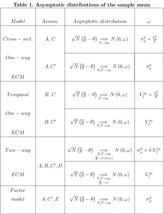
Two asymptotic theories are available for the cross-sectional and temporal one-way ECM. In the case of the two-way ECM, N and T must go to in…nity. The relative convergence rate between the two indexes, de…nes a continuum of asymptotic distributions. The factor model has a unique asymptotic dis-tribution when the two dimensions go to in…nity. The spatial dependence
possibly contained in f"itg for all the speci…cations, or in f iFtg for factor
model, vanishes when N and T go to in…nity.
Table 1. Asymptotic distributions of the sample mean
M odel Assum: Asymptotic distribution !
Cross sect: A; C pN y =) N !1N (0; !) 2 + 2" T One way A; C0 pN y =) N;T !1N (0; !) 2 ECM T emporal B; C pT y =) T !1N (0; !) V 1 f + 2 " N One way B; C0 pT y =) N;T !1N (0; !) V 1 f ECM T wo way pN y =) N;T !1 N T ! 2[0;1) N (0; !) 2 + :V1 f A; B; C0; D ECM pT y =) N;T !1 N T !1 N (0; !) Vf1 F actor model A; C0; E pN y =) N;T !1N (0; !) 2
1.4
Resampling Methods
In this section, we present the methods we use to resample panel data. These methods have in common that they resample the observed data yit. In
other words, their implementation do not depend on the choice of a particular structure for the data. However, of course the validity of each method will depend on the properties of the underlying data-generating process. In other words, we want to make inference that is robust to the panel data models described in the previous section without having to impose that model in resampling.
From our initial N T data matrix Y , bootstrapping will create a new matrix Y by resampling with replacement elements of Y: Statistics are com-puted on this pseudo-sample, and we repeat this operation B times. We use the sequence of B statistics generated by the bootstrap to make inference about the parameter :
A word on notation before presenting the resampling methods. Bootstrap quantities will be denoted by an asterisk. The probability measure induced by the resampling method conditional on Y is noted P . E () and V ar () are respectively the expectation and the variance associated with P .
Cross-sectional Resampling Bootstrap
For a N T matrix Y , cross-sectional resampling constructs a new N T matrix Y with rows obtained by resampling with replacement the rows of Y: In other words, we resample the vectors of T observations for each individual. As a consequence, conditionally on Y , the rows of Y are independent and identically distributed. yitcan only take one of the N values fyitgi=1;:::N, those
that were observed for some individuals at time t . Y takes the following form : Y (N;T )= 0 B B B B B @ y11= yi11 y12= yi12 ::: y1T = yi1T y21= yi21 y22= yi22 ::: y2T = yi2T ::: ::: :: ::: yN 1 = yiN1 yN 2 = yiN2 ::: yN T = yiNT 1 C C C C C A (4.1 )
where each of the indices (i1; i2; :::::; iN) is obtained by i.i.d. drawing
with replacement from (1; 2; :::::; N ). The mean of Y obtained by the cross-sectional bootstrap is denoted by ycros:
Block Resampling Bootstrap
This method is a direct generalization of block bootstrap methods de-signed for time series. Non-overlapping block bootstrap (NMB) (Carlstein (1986)), moving block bootstrap (MBB) (Kunsch (1989), Liu and Singh (1992)), circular block bootstrap (CBB) (Politis and Romano (1992)) and stationary block bootstrap (SB) (Politis and Romano (1994)) can be adap-ted to panel data. The idea is to resample in the time dimension blocks of consecutive periods in order to capture temporal dependence. All the obser-vations at each time period are kept together in the hope of preserving their dependence.
The block bootstrap resampling constructs a new N T matrix Y with columns obtained by resampling with replacement blocks of columns of Y: As a consequence, in this method, yit can only take one of the T values
fyitgt=1;:::T, those that were observed for individual i at some time t. The
mean of Y obtained by block bootstrap method is noted ybl. Y takes the
following form : Y (N;T )= 0 B B B B B @ y11= y1t1 y12= y1t2 ::: y1T = y1tT y21= y2t1 y22= y2t2 ::: y2T = y2tT ::: ::: :: ::: yN 1= yN t1 yN 2= yN t2 ::: yN T = yN tT 1 C C C C C A (4.2 )
The choice of (t1; t2; ::; tT)depends on the which block bootstrap method
is used in the time dimension. With the CBB bootstrap resampling, we have (t1; t2; :; tT) taking the form
1; 1+ 1; ::; 1+ l 1 | {z } block 1 2; 2+ 1; ::; 2+ l 1 | {z }; block 2 ::::::; [T =l]; [T =l]+ 1; ::; [T =l] + l 1 | {z } block [T =l]
where the vector of indices 1; 2; :::; [T =l] is obtained by i.i.d. drawing
with replacement from (1; 2; :::::; T ), l denoting the block length1.
Condi-tionally to Y , the blocks are i.i.d. and the properties of the original i.i.d. bootstrap are transferred to the blocks as statistical units. With the CBB there are T possible overlapping blocks of length beginning with each periods from t = 1.... to t = T 1; 2; ::; l | {z } block 1 2; 3; ::; l + 1 | {z } block 2 3; 4; ::; l + 2 | {z }; block 2 ::::k; k + 1; ::; k + l 1 | {z }; block k ::;T; 1; ::; l 1 | {z } block T : The CBB resampling on matrix Y is i.i.d. drawing with replacement of K = [T =l] blocks from the T possible blocks. Let ’s de…ne a new matrix Z, a transformation of the sample Y .
1The name Circular come from the fact that when
t > T l; the index of some
observations exceed T and are replace using the rule : T + t ! t, as if the original data are around a circle and after T we continue with the …rst observation t = 1:
Z (N;T ) = 0 B B B B B B B B @ z11 z12 ::: ::: ::: z1T ::: ::: :: ::: ::: ::: ::: ::: :: zik ::: ::: ::: ::: ::: ::: ::: ::: zN 1 zN 2 ::: ::: ::: zN T 1 C C C C C C C C A (4.3 ) where zik = 1l P t 2 block k
yit is for given unit i, the average of the
observa-tions of block k: The matrix Z will be useful to derive some theoretical result in the next section.
Others block bootstrap methods can also be accommodated in the time dimension to panel data. In this chapter the theoretical results will be given for the CBB. They remain valid for the NMB and the MMB because the three methods are asymptotically equivalent.
Double Resampling Bootstrap
This method is a combination of the two previous resampling methods. The term double comes from the fact that the resampling can be made in two steps. In a …rst step, one dimension is taken into account : from Y , an intermediate matrix Y is obtained either by cross-sectional resampling or block resampling. It turns out that the resampling is symmetric so it does not matter which dimension is resampled …rst. Then, another resampling is made in the second dimension : from Y the …nal matrix Y is obtained. If we resampled in the cross-sectional dimension in the …rst step, then we
resampled columns of the intermediate matrix in order to get our resampled matrix Y :2 The mean of Y is noted y .
Carvajal (2000) and Kapetanios (2008) have both suggested this double resampling in the special case where the block length is 1. They also analyze this resampling method by Monte Carlo simulations but give no theoretical support. The idea is that by drawing in one dimension, we preserve the de-pendence in that dimension in the …rst step. In the second step, we reproduce the properties in the other dimension by preserving the vectors drawn in the …rst step. Y takes the following form :
Y (N;T )= 0 B B B B B @ y11 = yi1t1 y12 = yi1t2 ::: y1T = yi1tT y21 = yi2t1 y22 = yi2t2 ::: y2T = yi2tT ::: ::: :: ::: yN 1= yiNt1 yN 2 = yiNt2 ::: yN T = yiNtT 1 C C C C C A (4.4 )
where the indices (i1; i2; :::::; iN) and (t1; t2; :; tT) are chosen as described
in the the two previous sub-sections. One important aspect of our analysis of double resampling is the properties of yit: Conditionally on the matrix [Y ] ; the elements of [Y ] have a particular dependence structure. In fact each element yit depends on the elements in its column and on its row. This link exists because elements on the same line belong to the same unit i and elements in the same column refer to the same period t. This structure of dependence and the validity of the bootstrap methods will be analyzed in the next section.
1.5
Bootstrap Validity
This section analyzes the properties of the bootstrap methods described in the previous section in the panel models described in section 2. A boots-trap method is consistent for the sample mean if the distance between the bootstrap distribution function and the sampling distribution of the statis-tic converges to 0 asymptostatis-tically. Since we have di¤erent (three) modes of convergence, we have three de…nitions of consistency. In order to avoid over-burdening the text, we will denote by !P
N T !1 the convergence in probability
under either case of asymptotic analysis : N …xed with T going to in…nity, T …xed with N going to in…nity, and …nally N and T going to in…nity simul-taneously. With this notation, we will say that the bootstrap is consistent if : sup x2R P pM y y x P pM y x !P N T !10 (5.1 ) with M 2 fN; T; NT g :
M is the scaling factor and depends on the panel model speci…cation. In the special case where the sample mean asymptotic distribution is available, consistency can be established by showing that the bootstrap sample mean has the same distribution. The next proposition expresses this idea.
Proposition 1 : Assume thatpM y =) L andpM y y =) L . If L and L are identical and continuous, then
sup
x2R
P pM y y x P pM y x !P
N T !10
To understand the behavior of the resampling schemes, it is convenient to decompose the error term. Using the matrix notation developed above, we can rewrite the data matrix Y as
Y = | {z }N 0T [ ] + 0 B B B B B @ 1 ::: 1 2 ::: 2 ::: :: ::: N ::: N 1 C C C C C A | {z } [ ] + 0 B B B B B @ f1 ::: fT f1 ::: fT ::: ::: ::: f1 ::: fT 1 C C C C C A | {z } [f ] + 0 B B B B B @ 1 2 ::: N 1 C C C C C A | {z } [ ] F1 ::: FT | {z } [F ] + 0 B B B B B @ "11 ::: "1T "21 ::: "2T ::: :: ::: "N 1 ::: "N T 1 C C C C C A | {z } ["] (5.2) = [ ] + [ ] + [f ] + [ ] [F ] + ["]
Thus, each line of the matrix [ ] contains T times the same value. Thus, if one were to resample [ ] in the cross-sectional dimension (i.e. drawing rows) and take the overall average would be equivalent to an i.i.d. resampling of i: Similarly, cross-sectional resampling is also equivalent to i.i.d. resampling of the factor loadings i:
On the other hand, the rows of the matrices [f ] and [F ] are identical. This means that cross-sectional resampling does not do anything and returns the original matrices [f ] and [F ] : E¤ectively, it treats (f1; :::; fT)and (F1; ::::; FT)
as constants. In other words, when doing cross-sectional resampling, each bootstrap observation can be decomposed as :
where i, i are i.i.d. draws.
The analysis for temporal block resampling is symmetrical. It is equivalent to block resampling on the time e¤ects f1; ::; fT and the factors F1; :::; FT.
However, it does not resample the individual e¤ects and factor loadings and teats them as constants. Hence, each bootstrap observation can be written as
yit;bl = + i+ ft;bl+ iFt;bl + "it;bl: (5.4 )
Finally, double resampling is the combination of the two previous me-thods. It is equivalent to the combination of i.i.d. resampling on the individual e¤ects ( 1; ::::; N) and factor loadings ( 1; ::::; N)and block resampling on
the time e¤ects (f1; ::::; fT) and factors (F1; ::::; FT) :
yit = + i + ft;bl+ iFt;bl+ "it: (5.5 ) Using the above expression, we can express the bootstrap means as :
ycros y = ( ) + F F + ["inter] " (5.6)
ybl y = fbl f + Fbl F + ["inter]bl " (5.7)
y y = ( ) + fbl f + Fbl F + " " (5.8) It must be noted that the centering eliminates ft in the case of
cross-sectional resampling and i in the case of temporal block resampling. It
follows immediately that cross-sectional resampling is inconsistent in the presence of temporal heterogeneity as it cannot reproduce it. Similarly, the temporal block resampling is inconsistent in presence of cross-sectional hete-rogeneity.
The particular dependence structure in Y , induces a particular form for the bootstrap variance of y as expressed by the following proposition.
Proposition 2 : 8 N; T , the double resampling bootstrap-variance is : V ar y = V ar z + 1 1 K V ar ycros + 1 1 N V ar ybl V ar y > 1 1 K V ar ycros (5.9) V ar y > 1 1 N V ar ybl
(5.9) gives the expression of the double resampling bootstrap mean va-riance. It is important to mention that these results are …nite sample pro-perties, holding without any assumption about yit. The …rst term V ar z
is the i.i.d. bootstrap mean variance for transformed data zik where in the
time dimension, we make the average of observations by block as described in (4.5). The second component of V ar y is the cross-sectional resampling bootstrap variance times 1 K1 and the third component is the block re-sampling bootstrap variance times 1 1
N . The two inequalities mean that
the double resampling bootstrap induces a greater variance than the cross-sectional resampling bootstrap and the block resampling bootstrap. That implies that in some cases the cross-sectional resampling bootstrap or the block resampling bootstrap could reject the null hypothesis while the double resampling bootstrap does not reject it. Inversely, if the double resampling bootstrap rejects the null hypothesis, there is no chance that a bootstrap method in one dimension does not reject it.
Another implication of (5.9) what happens in the particular case when the block length l = 1. (5.9) becomes :
V ar y = V ar y + 1 1 T V ar (yi:) N + 1 1 N V ar (y:t) T V ar y V ar y (5.10)
It is important to mention two things about inequality (5.10). First, the equality V ar y = V ar y holds in (5.10) when T = 1 (cross-section data) or N = 1 (time series). Second, (5.10) means that in …nite sample, the double resampling bootstrap induces a greater variance than the i.i.d. bootstrap. In particular the next proposition expresses what happens asymptotically when the double resampling bootstrap is applied to i.i.d. error term "it:
Proposition 3 : Under Assumption C, using the double resampling boots-trap with block length l=1 we have :
V ar pN T " !P
N;T !13. 2
" (5.11 )
In the absence of random heterogeneities, the double resampling induces a bootstrap-variance three times larger than i.i.d. bootstrap inducing a conser-vative con…dence interval.
Let’s introduce new assumptions about the error term "it:
Assumptions C”(idiosyncratic error)
C”1 : the scaled sample mean pM " (with M 2 fN; T g) converges in probability to zero.
C”2 : the empirical mean of squares of cross-section averagesN1 P
i
("i:)2
converges in probability to zero.
C”3 : the empirical mean of squares of temporal block averages[T =l]1 Pk(e:k)2
converges in probability to zero.
Assumption C” is a weaker version of assumption C. The …rst assump-tion ensures that the error term "it is asymptotically negligible : it is the
assumption C’). Assumption C”2 ensures that there is no cross-sectional hete-rogeneity remaining in "it . Assumption C”3 excludes temporal heterogeneity
in "it. [T =l] denotes the number of blocks in the time dimension and ek: the
average of the term "it in the block k for all the individuals as exposed in
(4.3).
Under assumption C” about the error term "it the next proposition
ana-lyzes the asymptotic behavior of " when the scaling factor is pN orpT.
Proposition 4 Under assumption C”, using the double resampling bootstrap we have : V ar pN " !P N;T !10 and V ar p T " !P N;T !10 (5.12 )
The implication of Proposition 4 is that when the scaling factor of y is pN or pT (presence of heterogeneities) the distribution of " does not appear in the asymptotic distribution of y . That means that the double resampling bootstrap method is valid under general spatial dependence. Thus validity of the bootstrap method will be focused of the components [ ] ; [f ] ; [ ] and [F ] :
Our validity proofs will imitate the procedure in Proposition 1. For each bootstrap method, by deducing the asymptotic distribution of the compo-nents of y y, using the appropriate scaling factor and comparing with the asymptotic distributions in Table 1, one can identify consistent and incon-sistent bootstrap for the di¤erent panel model speci…cations. The results are in the following proposition.
Proposition 5 : Consistency.
1 - In the presence of temporal heterogeneity, the cross-sectional bootstrap is inconsistent. sup x2R P pM ycros y x P pM y x 9P N T !10 with M 2 fN; T; NT g.
2 - In the presence of cross-sectional heterogeneity, the block bootstrap methods are inconsistent.
sup
x2R
P pM ybl y x P pM y x 9P
N T !10
with M 2 fN; T; NT g.
3 - In the presence of cross-sectional and/or temporal heterogeneity, under the assumption that l 1 + lT 1 = o (1) as T
! 1, the double resampling bootstrap is consistent when N and T go to in…nity
sup
x2R
P pM y y x P pM y x !P
N T !10
with M 2 fN; T g.
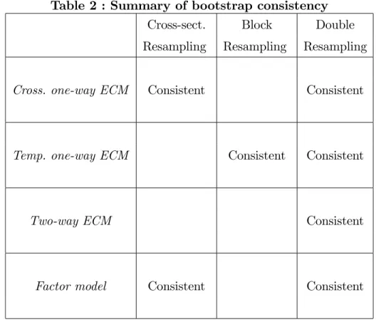
The condition about the convergence of l has a heuristic interpretation. If l is bounded, the block bootstrap method fails to capture the real dependence among the data. On the other hand, if l goes to in…nity at the same rate as T , there are not enough blocks to resample. The strength of the double resampling is to replicate the behavior of the main components of errors terms, without having to separate them. It is thus robust to the presence of these two types of heterogeneity and will allow for valid inference without having to make parametric assumptions. The consistency of the bootstrap methods for the di¤erent panel model speci…cations are presented in Table 2.
Table 2 : Summary of bootstrap consistency Cross-sect. Block Double Resampling Resampling Resampling
Cross. one-way ECM Consistent Consistent
Temp. one-way ECM Consistent Consistent
Two-way ECM Consistent
Factor model Consistent Consistent
1.6
Bootstrap Con…dence Interval
Once we have used the bootstrap to generate B pseudo samples, we can construct con…dence intervals for : In the literature, there are seve-ral bootstrap con…dence intervals. The percentile con…dence interval and the percentile-t con…dence intervals are the commonly used.
Bootstrap Percentile Interval
The …rst type of interval is based on the distribution of the bootstrap mean. For each pseudo-sample Yb , we compute the bootstrap-sample mean : yb and the centered statistic rb = yb y. The empirical distribution of these B realizations is :
b R (x) = 1 B B X b=1 I (rb x) (6.1 ) b
R is an approximation of the cumulative distribution function of the bootstrap-mean . The percentile con…dence interval of level (1 ) for the parameter is then constructed as
CI1 = y r1 =2; y r =2 (6.2 )
where r =2 and r1 =2 are respectively the =2-percentile and (1 =2)-percentile of bR : B should be chosen so that (B + 1) is an integer. When
b
R (x) is symmetric, r =2 = r1 =2 and a symmetric percentile interval is :
CI1 = C =2; C1 =2 (6.3 )
where C =2and C1 =2are respectively the =2-percentile and the (1 =2)-percentile of the empirical distribution function of yb b=1::B+1: This is a simple way of constructing a non-parametric con…dence interval.
Bootstrap Percentile-t Interval
Alternatively, one could build a percentile-t interval. These are often pre-ferred because they involve bootstrapping pivotal statistics (statistics that do not depend on nuisance parameters) and sometimes allow proving asymptotic re…nements (though we will not prove any such re…nement in this thesis).
To construct this type of intervals, we compute the t statistic on each pseudo-sample Yb :
tb = qyb y b V ar y
The empirical distribution of these B realizations is b G (x) = 1 B B X b=1 I (tb x) (6.5 )
A percentile-t con…dence interval of level (1 ) is
CI1 = y q b V ar y :t1 2; y q b V ar y :t 2 (6.6 )
where t =2 and t1 =2 are respectively the =2-percentile and (1 =2)-percentile of bG . The construction of these intervals resembles standard Wald-type statistics where one adds and subtracts a given quantile from the normal distribution (for example 1.96 for a 95% interval). The bootstrap is only used to compute the appropriate multiple of the standard error to add and subtract to the point estimate.
Bootstrap Interval Validity
The consistency of a bootstrap method implies the validity of the associa-ted percentile con…dence interval. If the asymptotic law is continuous, strictly increasing and symmetric, con…dence interval using directly the percentile of
yb is also valid3.
For the consistency of percentile-t con…dence interval, we need to show the consistency as expressed in (5.1) but applied to studentized statistics. The next proposition analyzes the case of the double resampling bootstrap.
Proposition 6 In the presence of cross-sectional and/or temporal heteroge-neity, under assumptions A - E and the assumption that l 1 + lT 1 = o(1) as T ! 1; we have : sup x2R P 0 @q y y b V ar y x 1 A P 0 @qy b V ar y x 1 A P ! N;T !10 (6.7 )
where bV ar y = V ar y and bV ar y is the analog of V ar y on the pseudo-sample Y :
The intuition is that with the consistency as de…ned in (5.1), V ar y is asymptotically equivalent to V ar y thus it is a consistent estimator. In the bootstrap world the analog of V ar y is a good choice to studentize y y : Like this the consistency with tb is also given, justifying the use of percentile-t con…dence interval. Similar results are given with the cross-sectional resampling bootstrap and the block resampling bootstrap using respectively bV ar y = V ar ycros , bV ar y = V ar ybl and their analogs in the bootstrap world.
The consistency of the double resampling bootstrap percentile-t con…-dence interval, as de…ned in (5.1), has been provided when N and T go to in…nity. A question arises : the validity of the double resampling bootstrap method for inference when only one dimension goes to in…nity. The next proposition compare the percentile-t con…dence intervals.
Proposition 7 For N and T large enough CI1cros 2 CI1 (6.8) CI1bl 2 CI1 (6.9) where CI1cros = y q V ar ycros :t1cros 2 ; y q V ar ycros :t cros 2 CI1bl = y q V ar ybl :t1bl 2; y q V ar ybl :t bl 2 CI1 = y q V ar y :t1 2; y q V ar y :t 2
For the validity of con…dence interval associated to cross-sectional (resp. block) resampling bootstrap we need N (resp. T ) to go to in…nity. When the other dimension is large enough, the Proposition 7 ensures that the valid percentile-t con…dence interval associated belong to the double resampling bootstrap percentile-t con…dence interval that is valid even if the second dimension is …xed, in the sense that the level is controlled.
Pr 2 CI1 1 (6.10 )
With all the theoretical results in hand, in the next section we will see the behavior of the bootstrap methods in …nite sample, using simulations.
1.7
Simulations
This section presents results from a small simulation experiment to illus-trate our theoretical results. The data generating process is (2 :1 ) and (2 :2 ) :
The individual e¤ects are standard normal and independent across units :
i i:i:d:N (0; 1) ;
while both the time e¤ect and common factor are AR (1) process with para-meter 0.5 :
ft = ft 1+ $t
Ft = Ft 1+ t
t; $t i:i:d:N 0; 1 2
= 0:5
The factor loadings are standard normal :
i i:i:d:N (0; 1)
and the idiosyncratic errors are also standard normal : "it i:i:d:N (0; 1) :
Six panel dimensions are considered : (N; T ) = (10; 10) ; (30; 30) ; (60; 60) ; (10; 6)and (6; 10). Temporal resampling is carried out with the Circular Block Bootstrap (CBB) with block length l = 2; 2; 3; and 4 respectively for T = 6; 10, 30 and 60. For each bootstrap resampling scheme, B is equal to 999 and the number of simulations is 1000.
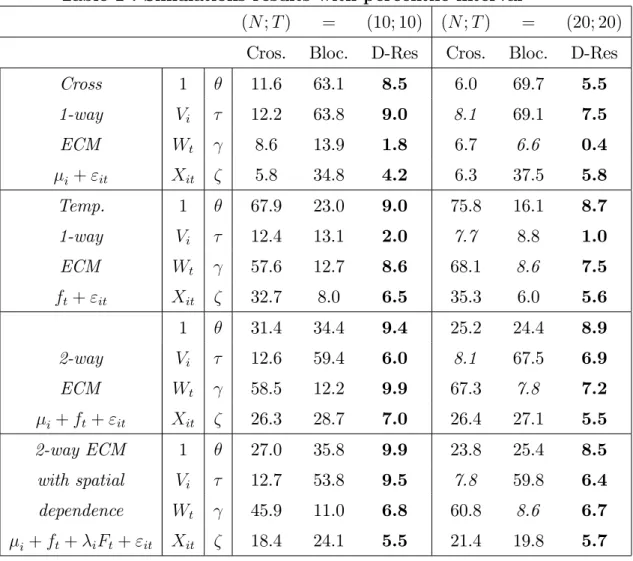
Tables 3 gives rejection rates for a two-tailed test for the null hypothesis that = 0at nominal level 5%. The rejection rates close to 5% are presented in bold.
The simulations con…rm the theoretical results. In particular, we see that the double resampling performs well for all models considered : the cross-sectional and temporal one-way ECM, the two-way ECM and the factor
model. The other bootstrap schemes fail for at least one model. The cross-sectional bootstrap performs well with one-way ECM and factor model, but cannot reproduce temporal heterogeneity. Similarly, the block bootstrap per-forms well with temporal one-way ECM, but it cannot provide reliable infe-rence in the cross-sectional one-way or two-way ECM or the factor model. The implication of Proposition 2 is visible in Table 3 : for any sample size, the double resampling bootstrap induces a rejection rate smaller than the block resampling bootstrap and the cross-sectional resampling bootstrap rejection rates.
1.8
Conclusion
This chapter considers bootstrap resampling for panel data..It is shown that double resampling that combines cross-sectional and block resampling is valid for panel data models with cross-sectional and/or temporal heteroge-neity. Some weak forms of spatial and serial dependence in the idiosyncratic errors can even be allowed for if both the cross-sectional and time dimensions are large. On the other hand, resampling only in the cross-sectional dimen-sion is not valid in presence of temporal heterogeneity, and block resampling in the time dimension only is not valid in the presence of cross-sectional heterogeneity.
There are two important advantages of the methods proposed in this paper. The …rst one is that double resampling is able to replicate the behavior of the error term, without having to separate it into components (which would require making strong parametric assumptions). Secondly, the bootstrap has the nice advantage of avoiding having to choose among multiple asymptotic approximations.
There are several directions in which the current work can be extended to be made more realistic. One would be to relax some of the strong assumptions that were made on the individual e¤ects. Also, one would like to introduce regressors in the model. This will be the subject of the next chapter.
Table 3 : Simulation results with percentile-t M odels (N ;T) Cross. Block D-Res
(10 ;10) 5.5 60.2 4.2 Cross sectional (30 ;30) 4.9 73.1 4.4 (60 ;60) 5.2 79.8 5.1 One way (10 ;06) 6.9 57.9 5.1 ECM (06 ;10) 10.8 62.6 6.8 (10 ;10) 58.8 11.8 6.6 T emporal (30 ;30) 73.1 6.4 5.7 (60 ;60) 81.1 6.3 5.5 One way (10 ;06) 59.1 17.7 10.7 ECM (06 ;10) 57.1 11.4 5.0 (10 ;10) 20.5 23.5 5.5 T wo way (30 ;30) 18.6 20.3 5.2 (60 ;60) 17.5 18.6 5.3 ECM (06 ;10) 19.2 28.4 5.6 (10 ;06) 19.5 28.1 6.5 (10 ;10) 8.3 52.9 4.1 (30 ;30) 6.4 65.1 5.1 F actor (60 ;60) 4.6 75.3 4.1 model (06 ;10) 10.7 48.7 5.1 (10 ;06) 9.5 51.1 4.5
APPENDIX
Proposition 8 : Assume that A2 holds, assume also that l 1+ lT 1 = o (1)
as T ! 1;, using NMB, MBB or CBB, we have sup x2R P pT fbl f x P pT f 0 x !P T !10 p T fbl f =) T !1N 0; V 1 f
Proof. [Proof of Proposition 8] Under the assumptions and the convergence rate imposed to l, a demonstration of the consistency of MMB, NMB and CBB for time series, can be seen for example in Lahiri (2003), p. 55 .
Classical Asymptotic Distributions Cross-sectional one-way ECM
a) T is …xed. yi: are i.i.d. with E (yi:) = and V ar (yi:) = 2 + 2"
T .
Applying a standard CLT, the result follows. b) p N y = p1 N N X i=1 i+ p N " 1 p N N X i=1 i =) N !1N 0; 2 by CLT and pN " P ! N;T !10( Assumption C’)
Temporal one-way ECM a)T ! 1 p T y = p1 T T X t=1 ft ! + p1 T T X t=1 ":t ! 1 p T T X t=1 ft ! =) T !1N 0; V 1 f (Proposition 6 ) 1 p T T X t=1 ":t ! =) T !1N 0; 2 " N thus p T y =) T !1N 0; V 1 f + 2 " N b)N; T ! 1 p T y = p1 T T X t=1 ft ! +pT " p N " !P N;T !10 ( C’) thus p T y =) N;T !1N 0; V 1 f Two-way ECM a)NT ! 2 [0; 1) p N y = p1 N N X i=1 i+ p N p T 1 p T T X t=1 ft ! +pN " 1 p N N X i=1 i =) N !1N 0; 2 by CLT; 1 p T T X t=1 ft ! =) N;T !1N 0; V 1 f . p N " !P N;T !10 ( C’)
The result follows4. 4When the vector(X
n; Yn)
0
distribu-b)NT ! 1 p T y = p T p N 1 p N N X i=1 i ! + p1 T T X t=1 ft ! +pT " p N " !P N;T !10; p T p N 1 p N N X i=1 i ! m:s: ! N;T !10 1 p T T X t=1 ft ! =) T !1N 0; V 1 f
The result follows.
Factor Models p N y = p1 N N X i=1 i+ 1 p N N X i=1 i ! 1 T T X t=1 Ft ! +pN " 1 p N N X i=1 i =) N !1N 0; 2 1 p N N X i=1 i ! 1 p T T X t=1 Ft ! =) N;T !1 N 0; 2 N 0; V1 f thus 1 p N N X i=1 i ! 1 T T X t=1 Ft ! m:s: ! N;T !10 p N " !P N;T !10 ( C’) and we have p N y =) N;T !1N 0; 2
tion of any linear combination of the elements of the vector (in particular the sum) can be deduced. The fact that Xn and Ynare independent and converge to a normal distribution,
Proof.[Proof of Proposition 1] y and y having the same asymptotic distri-bution, implies that jP (::) P (::)j converges to zero. Under the continuity assumption, uniform convergence is given by the Pólya theorem (Pólya (1920) or Ser‡ing (1980), p. 18)
Proof. [Proof of Proposition 2] An analysis of variance gives :
Using CBB, there is the time dimension, K blocks are chosen from T possible blocks. The bootstrap-mean y rewritten as
y = 1 N T N X i=1 T X t=1 yit = 1 N K N X i=1 K X k=1 zik where zik = 1 l X t 2 block k yit V ar y = V ar z = 1 N KV ar (zit )+ 1 (N K)2 X (i;k)6= X (j;s) Cov zik; zjs zik can take any of the N T values of elements of [Z] with probability 1=N T then the expectation and the variance are identical to those obtained with i.i.d. bootstrap accommodated to panel data [Z] : E (zit) = E (zit) ; V ar (zit) = V ar (zit).
For i 6= j and k 6= s, Cov zik; zjs = 0
1 (N K)2 X (i;k)6= X (j;s) Cov zik; zjs = 1 (N K)2 K X k=1 X i6= X j Cov zik; zjk + 1 (N K)2 N X i=1 X t6= X s Cov (zik; zis)
Cov zik; zjk = 1 N2T K X k=1 N X i=1 N X j=1 zikzjk 1 N T N X i=1 T X k=1 zik !2 = 1 T T X t=1 1 N N X i=1 zik !2 1 N T N X i=1 K X k=1 zik !2 = 1 T T X k=1 (z:k)2 1 T T X k=1 z:k !2 = V ar (z:k) Similary Cov (zik; zis) = V ar (zi:) zi: = 1 K K X k=1 zik = 1 K K X k=1 " 1 l X t 2 block k yit # zi: = 1 Kl T X t=1 yit = 1 T T X t=1 yit = yi:
There are T (N2 N )possibilities of Cov z
ik; zjk . There are N (T2 T )
possibilities of Cov (zik; zis)then : V ar y = V ar (zik) N T + 1 1 T V ar (zi:) N + 1 1 N V ar (z:k) T V ar y = V ar z + 1 1 T V ar (yi:) N + 1 1 N V ar (z:k) T V ar y = V ar z + 1 1 T V ar ycros + 1 1 N V ar ybl V ar y > 1 1 T V ar ycros V ar y > 1 1 N V ar ybl
Proof. [Proof of Proposition 3] Variance decomposition in the proof of Pro-position 2 gives : V ar pN T " = V ar ("it)+ 1 1 T [T:V ar ("i:)]+ 1 1 N [N:V ar (":t)] V ar ("it) !P N T !1 2 " ; [T:V ar ("i:)] P ! N !1 2 " ; [N:V ar (":t)] P ! T !1 2 " therefore V ar pN T " !P N;T !13: 2 "
Proof. [Proof of Proposition 4]
V ar pN " = E pN " 2 hE pN " i2 = E pN "
2 hp
N "i
2
By assumption pN " ! 0 thusP hpN "i2 ! 0: Let’s study now the behaviorP of E pN "
2
:
The block size is l and we have K blocks.
" = 1 N T P i P t "it = 1 N K P i P k eik = 1 N K P i P k eit i k
where eik denote for given i the average of observations in the block k:
i M ultinomial N; p1 = p2 = :::::: = pN = N1 and
k M ultinomial K; p1 = p2 = :::::: = pK = 1 denotes the
num-ber of potential block to resample from Y: For the case of CBB = T i
(resp. k)denotes how much time individual i (respectively block k)appears in the pseudo-sample Y : i is independent of k and both are indepndent
of the observations : E pN " 2 = N E 1 N K P i P k eik i k 2 = N E 1 N K 2 P i P j P k P s eikejs i j k s ! = N 1 N K 2 P i P j P k P s eikejsE ( i j k s) = N 1 N K 2 P i P j P k P s eikejsE ( i j) E ( k s) if i = j, E ( i j) = E ( 2i) = V ar ( i) + [E ( i)] 2 = N pi(1 pi) + N pi = N N1 1 N1 + 1 = 1 N1 + 1 if i 6= j E ( i j) = Cov ( i j) + E ( i) E ( j) = N pi pj+ N pi N pj = N1 + 1 = 1 N1 if k = s, E ( k s) = E 2 k = V ar ( k) + [E ( k)] 2 = K pk(1 pk) + [K pk]2 = K T1 1 T1 + K T1 2 = 1l 1 T1 + 1l 2 = 1l 1l T1 + 1 if k 6= s E ( k s) = K pk ps+ K pk K ps = K 1 T 1 T + K 1 T K 1 T = 1 l 1 T + 1 l 2 = 1l 1l T1
E pN " 2 = N 1 N K 2 P i P j P k P s eitejsE ( i j) E ( k s) = N 1 N K 2 P i P j P k P s eikejs 1 1 N 1 l 1 l 1 T +N 1 N K 2 P i P k P s eikeis+ N 1 N K 2 P i P j P k eikejk 1 l = N 1 1 N 1 l 1 l 1 T 1 N K P i P k eik 2 +N 1 K 2 P k 1 N P i eik 2 1 l +N 1 N 2 P i 1 K P k eik 2 1 N K P i P t eit = 1 N T P i P t "it " 1 K P k eik = 1 T P t "it "i:; thus E pN " 2 = N 1 1 N 1 l 1 l 1 T " 2 + 1 N P i ["i:] 2 + N K 1 l 1 K P t [":t] 2 = 1 1 N 1 l 1 l 1 T hp N "i | {z } P !0 2 + 1 N P i ["i:]2 | {z } P !0 + N T 1 K P k [":k]2 | {z } P !0 P ! 0 thus V ar pN " ! 0P Similary,
E pT " 2 = T 1 1 N 1 l 1 l 1 T " 2 + 1 N P i ["i:]2+ N K 1 l 1 K P t [":t]2 = 1 1 N 1 l 1 l 1 T hp T "i | {z } P !0 2 + T N 1 N P i ["i:] 2 | {z } P !0 + 1 K P k [":k] 2 | {z } P !0 P ! 0 thus V ar pT " ! 0:P
Proof.[Proof of Proposition 5] With the cross-sectional resampling, the cen-tering eliminates the temporal heterogeneity fftg. Its behavior does not
ap-pear neither in …nite sample properties nor in the asymptotic distribution and therefore causes inconsistency. With block resampling, the centering elimi-nates the cross-sectional heterogeneity f ig ; therefore insconsistency. With
the double resampling, all the properties demonstrated for the i.i.d. bootstrap or for the various block bootstrap methods are transferred to the appropriate errors terms without restriction. With the di¤erent speci…cations, the consis-tency or the inconsisconsis-tency holds comparing the bootstrap asymptotic distri-bution and the classic asymptotic distridistri-bution, according Proposition 1.
Proof. [Proof of Proposition 6] We have already the consistency of Proposi-tion 5 in hand.
with bV ar y = V ar y and bV ar y is the analog of V ar y on the pseudo-sample Y ; the proposition 4.1 of Shao and Tu (1995) ensures that the consistency of Proposition 5 implies the result in Proposition 6.
Proof. [Proof of Proposition 7] For the three bootstrap methods we have : sup
x2RjP (tb
x) (x)j !P
N T !10
For N andT large enough, t cros
1 2 t1bl2 t1 2 > 0 and t2cros t2bl t2 < 0 V ar y V ar ycross V ar y V ar ybl CI1cros = y q V ar ycros :t1cros 2 ; y q V ar ycros :t cros 2 2 y q V ar y :t1cros 2 ; y q V ar ycros :t cros 2 y q V ar y :t1 2; y q V ar ycros :t 2 = CI1 Similary CI1bl 2 CI1