Science Arts & Métiers (SAM)
is an open access repository that collects the work of Arts et Métiers Institute of
Technology researchers and makes it freely available over the web where possible.
This is an author-deposited version published in: https://sam.ensam.eu
Handle ID: .http://hdl.handle.net/10985/19941
This document is available under CC BY license
To cite this version :
Ruben IBANEZ, Pierre GILORMINI, Elias CUETO, Francisco CHINESTA - Numerical
experiments on unsupervised manifold learning applied to mechanical modeling of materials and
structures - Comptes Rendus. Mécanique - Vol. 348, n°10-11, p.937-958 - 2020
Any correspondence concerning this service should be sent to the repository
Administrator : [email protected]
Numerical experiments on unsupervised
manifold learning applied to mechanical
modeling of materials and structures
Ruben Ibanez
a, Pierre Gilormini
a, Elias Cueto
band Francisco Chinesta
∗, aaPIMM lab, Arts et Metiers Institute of Technology, 151 Boulevard de Hôpital, 75013
Paris, France
bAragon Institute of Engineering Research, Universidad de Zaragoza, Maria de Luna
s/n, 50018 Zaragoza, Spain
E-mails: [email protected] (R. Ibanez), [email protected]
(P. Gilormini), [email protected] (E. Cueto), [email protected] (F. Chinesta)
Abstract. The present work aims at analyzing issues related to the data manifold dimensionality. The interest
of the study is twofold: (i) first, when too many measurable variables are considered, manifold learning is expected to extract useless variables; (ii) second, and more important, the same technique, manifold learning, could be utilized for identifying the necessity of employing latent extra variables able to recover single-valued outputs. Both aspects are discussed in the modeling of materials and structural systems by using unsupervised manifold learning strategies.
Keywords. Nonsupervised manifold learning, State variables, Dimensionality reduction, k-PCA, Structural
analysis, Material constitutive equations.
1. Introduction
Recently, data-driven description of materials has been gaining popularity. Many complex ma-terial behaviors resisting traditional modeling procedures, or that are too complex from a mi-crostructural viewpoint, are approached by using data-based descriptions. Different approaches are being considered. Among them include those based exclusively on measured data, others that extract the manifolds related to data, and others that attempt to enforce thermodynamic and thermomechanical consistency. The interested reader can refer to [1–7] and the numerous references therein. This work focuses on techniques based on the use of manifolds and their as-sociated manifold learning procedures for extracting them from the available data.
Figure 1. Multidimensional data on one- (left), two- (center), and three-dimensional
(right) manifolds embedded inRD.
In general, data involve many dimensions. Consider first a sequence of three-dimensional (3D) fields defined in a domainΩ ⊂ R3partitioned into D voxels. Each of these fields contains many data, one datum at each voxel. Each field can be represented as a point in a vector space of dimension D (the number of voxels), where we can presume each of the D coordinate axes as reporting the value that the field of interest takes in the associated voxel. Thus, each field becomes a point in that high-dimensional space of dimension D,RD. If important correlations exist among the different fields, these points are expected to be distributed on a low-dimensional subspace embedded in the D-dimensional space. Techniques aiming at extracting these reduced subspaces, the so-called slow manifolds, sketched in Figure 1, are key tools for manipulating data and extracting their hidden information.
Thus, data define in general slow manifolds embedded in very large vector spaces due to the significant hidden correlations among them. The number of uncorrelated explicative dimensions usually becomes much smaller than the a priori assumed dimension of the space for accommo-dating the data. The extraction of these slow manifolds can be successfully accomplished by using linear and nonlinear dimensionality reduction techniques such as principal component analysis (PCA) in the linear case and its nonlinear counterparts (`PCA, kernel-based PCA [k-PCA], LLE, tSNE, etc.) [8–12].
These techniques can be applied to several physical systems. Moreover, when the slow mani-fold is determined, the solution at any point on it can be computed very accurately from a sim-ple interpolation of neighboring data on the manifold [13], enabling almost real-time predictions and the associated real-time decision-making.
However, extracting knowledge from data associated with an existing but hidden model requires the following:
• identifying the manifold intrinsic dimension, • discovering hidden parameters,
• discarding useless parameters, and
• discovering the models originating the data.
These questions are addressed, illustrated, and discussed in the present work in a purely methodological manner, aiming at illustrating the key concepts that could open numerous future possibilities in the field of mechanics of materials, processes, structures, and systems.
In our previous works, we addressed problems involving thousands of dimensions [13–16], proving that despite the apparent richness in many cases, the embedding regards a relatively low-dimensional space. However, in most of the problems that we have treated until now, their complexity prevented fine analyses of their solutions. The present paper, which is purely methodological, considers simple problems defined in low dimensions, with known solutions
being easily visualizable, for facilitating an analysis and discussion. Of course, and as proved in the works just referred to, all the methodologies apply to multidimensional settings.
2. Unsupervised manifold learning
Let us consider a vector y ∈ RD containing experimental or synthetic data from measurements or numerical simulation. These results are often referred to as snapshots. If they are obtained by numerical simulation, they consist of nodal values of the essential variable. Therefore, these variables will be somehow correlated and, notably, there will be a linear transformation W defining the vectorξ ∈ Rd, with d < D, which contains the still unknown latent variables such that
y = Wξ. (1)
The D × d transformation matrix W, which satisfies the orthogonality condition WTW = Id, is the main ingredient of the PCA and can be computed as detailed in Appendix A from the covariance matrix associated with a number (M) of snapshots y1, . . . , yM, which constitute the
columns of matrix Y.
While PCA works with the covariance matrix (i.e., YYT), multidimensional scaling (MDS) works with the Gram matrix containing scalar products (i.e., S = YTY) as described in Appendix A.
On the other hand, the k-PCA is based on the fact that data not linearly separable in D dimensions could be linearly separated if previously projected to a space in Q > D dimensions. However, the true advantage arises from the fact that it is not necessary to write down the analytical expression of that mapping as described in Appendix A.
3. An illustrative structural mechanics case study
Consider first a hypothetical mechanical system consisting of a prismatic beam whose three dimensions, height, width, and length, are denoted, respectively, by h, b, and L, all of them being measurable quantities. In what follows, we consider a particular output P that constitutes also a measurable quantity (buckling critical load, etc.) assumed related to those parameters from an existing but actually hidden model even if in what follows we will consider hypothetical, and most of the time, unphysical models.
Thus, we consider a set of data composed ofMmeasures yi = {hi, bi, Li, Pi}, i = 1,...,M, with
hi, bi, and Libeing randomly chosen from a uniform probability distribution in their respective intervals of existence,Ih,Ib, andIL, respectively, defined from the following:
Ih= [hmin, hmax] Ib= [bmin, bmax] IL= [Lmin, Lmax]. (2) Without any other pre-existing knowledge, one expects the output depending on the three ge-ometrical parameters (i.e., P = P(h,b,L)). In what follows, we consider three different scenarios.
3.1. Output depending on a single parameter
In this section, we assume a quite simple model that relates the output to a single parameter,
P = αb, α ∈ R+, (3)
where α = 1000 in the numerical tests carried out. We perform M = 1000 measures, where Ih∈ [0.1, 0.2], Ib∈ [0.15, 0.2], and IL∈ [1, 1.5].
Figure 2. Eigenvaluesλ ∈ [λ110−6,λ1].
The measures constitute a set ofM= 1000 points in R4on which the k-PCA is applied by using the Gaussian kernel
κ(yi, yj) = exp
−kyi −yj k
2
2β2 , (4)
whereβ = 10.
Figure 2 depicts the highest eigenvalues among M resulting from the k-PCA, those lying between the highest valueλ1and 10−6λ1.
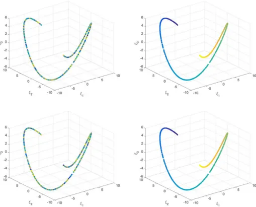
The slow manifold associated withξ is represented by selecting the first three reduced coor-dinates (ξ1,ξ2,ξ3) as shown in Figure 3, where its one-dimensional (1D) intrinsic dimension is
noted. This result was expected from the considered model expressed by (3). The points on the slow manifold are colored depending on the values of h, b, L, and P , evidencing that b constitutes the latent variable and that the output P scales (visually) linearly with it.
The process of coloring the data points in the embedded manifold deserves some additional comments due to the fact that this is used in all the analyses reported in the present paper. Man-ifold learning techniques look for a low-dimensional manMan-ifold defined by data points. As soon as the slow manifold is extracted, the different data points can be mapped on it. This visualization is only possible when the number of dimensions allows a simple graphical representation (as is the case for the problems addressed in the present paper). Then, these points can be colored de-pending on the value of the different initial coordinates, and one expects that if there is a corre-lation (direct or inverse and linear or nonlinear) between the initial and reduced coordinates, the colors must exhibit a certain grading.
Even if this analysis seems quite dependent on the low dimensionality of the embedding, in higher dimensional embeddings, the analysis can be performed by using local statistics. Thus, by considering a data point in the slow manifold and its closest neighbors, a local statistical analysis can be easily performed with the standard deviation indicating the dispersion of the data (equivalent to the local dispersion of colors).
One could be slightly surprised by the nonlinearity that the manifold exhibits despite the linearity of model (3). This nonlinearity is an artifact of the nonlinear kernel (4) used. As the model is linear, one could expect the ability of the PCA to address the problem at hand. For this purpose, it suffices transforming the kernel into its linear counterpart, giving rise to the PCA
Figure 3. Slow manifold in the 3D space defined by the first reduced coordinates (ξ1,ξ2,ξ3).
Each point is colored according to the value of the coordinate h (top left), b (top right), L (bottom left), or P (bottom right).
Figure 4. Slow manifoldξ when considering the PCA linear dimensionality reduction. Each
point is colored according to the value of the variable b.
In this case, as expected, a single nonzero eigenvalue results, and consequently the dimension of the reduced space becomes one (i.e.,ξ = ξ). The associated manifold is depicted in Figure 4.
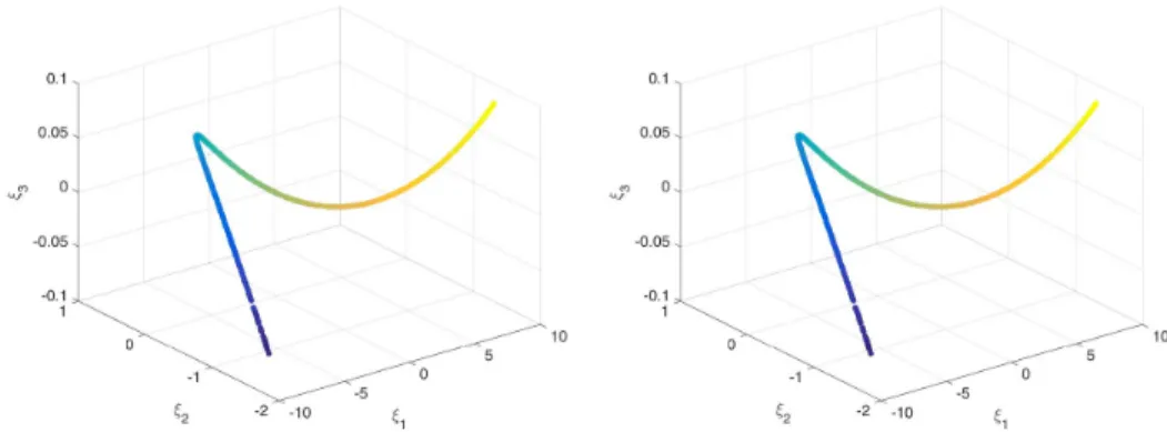
Now, we consider a slightly different model, again depending on a single variable but in a nonlinear manner, according to
Figure 5. Slow manifold in the 3D space defined by the first three reduced coordinates
(ξ1,ξ2,ξ3). Each point is colored according to the value of the coordinate h (left) or P (right).
Figure 6. Slow manifold in the 3D space defined by the first three reduced coordinates
(ξ1,ξ2,ξ3). Each point is colored according to the value of the coordinate L (left) or P (right).
where againα = 1000. Figure 5 depicts the 1D slow manifold, where points are colored according to the values of the variables h and P . Here, even if the direct relation can be noted, its nonlinear-ity is much less evident to visualize.
Finally, we consider the model
P = α
L2, (7)
whereα = 1000. Figure 6 depicts the 1D slow manifold, where points are colored according to the values of the variables L and P to emphasize the inverse relation between them.
3.2. Output depending on two parameters
In this section, we consider a model involving two of the three variables, in particular,
P = αh
3
L2, (8)
whereα = 1000.
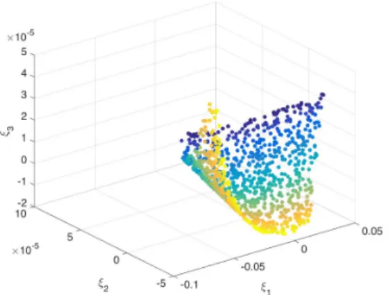
Figure 7 depicts the two-dimensional (2D) slow manifold, where points are colored according to the values of variables h, b, L, and P . Here, the direct and inverse effects of h and L with respect to P can be noted as well as the fact that parameter b seems, and in fact is, useless.
Figure 7. Slow manifold in the 3D space defined by the first three reduced coordinates
(ξ1,ξ2,ξ3). Each point is colored according to the value of the coordinate h (top left), b (top
right), L (bottom left), or P (bottom right).
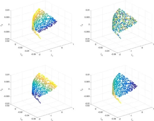
3.3. Identifying hidden variables
The previous case studies revealed the ability to extract the intrinsic dimensionality of the slow manifold as well as the possibility to identify useless parameters. The present case addresses a very different situation in which the model involves the three variables in the discussed case, h,
b, and L. However, only two of them were measured, namely h and L with the output P , with b
remaining inaccessible. Thus, we have
P = αbh
3
L2 , (9)
whereα = 1000. Therefore, theM= 1000 collected data yi, i = 1,...,M, reads as yi= {hi, Li, Pi} ∈ R3. Figure 8 depicts the reduced points (ξ1,ξ2,ξ3), which as can be seen are distributed in a
domainω ⊂ R3. However, no dimensionality reduction is noted, and the embedding remains 3D. A direct consequence is that many values of the output P exist for the same values on the measured inputs h and L, related to the different values of b, which affect the output P. However, as b is not measured, its value is not considered in the data points.
Such a multivalued output does not represent any conceptual difficulty. It indicates that even if both variables participate in the output, there may be others that were not considered or those considered may be useless for explaining the output.
Figure 8. Reduced representationξi∈ R3of the data yi∈ R3, where the reduced points are colored according to the value of the output P .
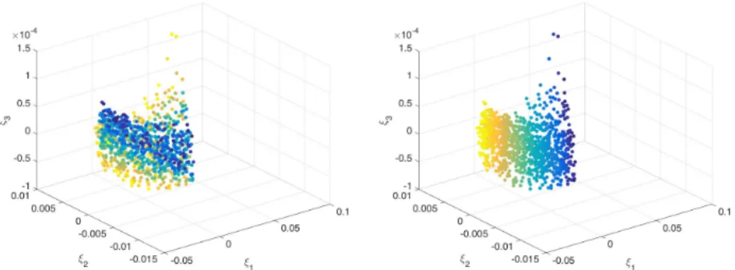
Figure 9. Reduced points colored according to the values of the coordinates h (left) and L
(right).
To conclude about the pertinence of these variables with respect to the considered output, we consider coloring the reduced data depending on the h and L values (refer to Figure 9). We compare them with the one where the color scales with the output P reported in Figure 8.
Thus, one could conclude that both variables h and L are relevant for explaining the output P . If we assume that the output P should be univocally explained from a small number of variables, clearly only two variables (here h and L) are not sufficient. One extra dimension suffices for recovering a single-valued output, that is, considering the reduced points in four dimensionsR4. As visualizing things in four dimensions is quite a difficult task, for the sake of clarity in the exposition, in what follows, we propose addressing a simpler model involving lower dimensional spaces.
We consider the simpler model
P = αbh3, (10)
whereα = 1000. However, theM= 1000 collected data yi, i = 1,...,M, only deal with h and P , (i.e.,
yi= {hi, Pi} ∈ R2).
Figure 10 depicts the dataset yi= {hi, Pi}, where it can be noted that many values of the output
P are found for the same value of the variable h.
For univocally expressing the output P , we consider again the k-PCA. We compute the reduced dataset in a 3D space by considering the first three coordinates (ξ1,ξ2,ξ3), while coloring these
Figure 10. Dataset yi= {hi, Pi}, i = 1,...,M.
Figure 11. Reduced points colored according to the values of the coordinates h (left) and P
(right).
points with respect to h, to prove that h represents an explanatory variable, or with respect to P (refer to Figure 11). Figure 12 depicts the same manifold but now colored by using the hidden variable b, which proves that it contributes to explaining the output P and constitutes the hidden variable. Even if we just proved that a latent variable exists, and that it corresponds to b, as in practice we ignore this fact, we never measure the quantity b. Furthermore, it is even possible that we ignore its existence; the proposed procedure is only informative but not constructive.
Obviously, there is no unique choice. The same behavior is obtained by coloring the reduced dataset with respect to any function bphq, where p, q ∈ R. Thus, any measurable variable ensur-ing such a uniform color gradensur-ing could be used as the latent variable for constructensur-ing the model. There are an infinite number of possibilities but with certain constraints; in the present case, it must involve b.
To conclude this section, we address a similar but more complex situation. We consider now the richer model (9) withα = 1000. TheM= 1000 collected data yi, i = 1,...,M, only deal with the input variable h and the output P (i.e., yi = {hi, Pi} ∈ R2), where two variables, b and L, involved in model (9) remain hidden.
Figure 13 depicts the dataset yi= {hi, Pi}, where again it can be noted that many values of the output P are found for the same value of the variable h.
For univocally expressing the output P , we consider again the k-PCA. We compute the reduced dataset in a 3D space by considering again the first three coordinates (ξ1,ξ2,ξ3) while coloring
Figure 12. Reduced points colored according to the value of the output b.
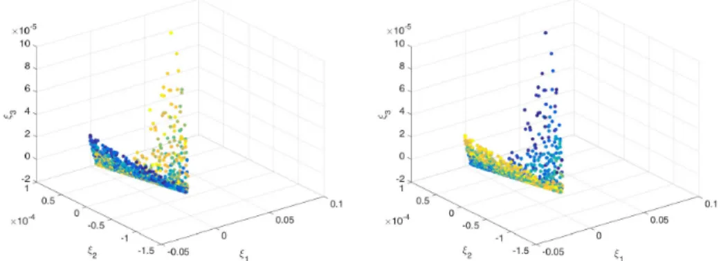
Figure 13. Dataset yi= {hi, Pi}.
these points with respect to h to prove that h represents an explanatory variable of the output P as Figure 14 proves. Figure 15 clearly reveals that by coloring the reduced points with respect to the two variables b and L taken solely, they do not represent the unique hidden variable able to explain using h the output P . The hidden latent variable according to model (9) should combine
b and h. Figure 16 proves that the combined parameter b/L2perfectly works when compared with the manifold colored with respect to the output P .
It is important to note that the latent variable must involve the term b/L2up to any power and eventually a multiple of any power of h.
3.4. Discussion
The previous numerical experiments allow drawing a conclusion on the ability of unsupervised manifold learning techniques for identifying useless data and the existence of latent variables.
The procedure is based on the ability of embedding high-dimensional data in a low-dimensional space, where the dimension represents an approximation of the inherent dimen-sionality of the data.
Figure 14. Reduced points colored according to the value of the coordinate h.
Figure 15. Reduced points colored according to the values of the variables b (left) and L
(right).
Figure 16. Reduced points colored according to the values of the variables b/L2(left) and
P (right).
When the expected dimensionality reduction does not occur and the k-PCA reveals univocally that an extra dimension is required to accommodate the data, this indicates the existence of a hidden latent variable.
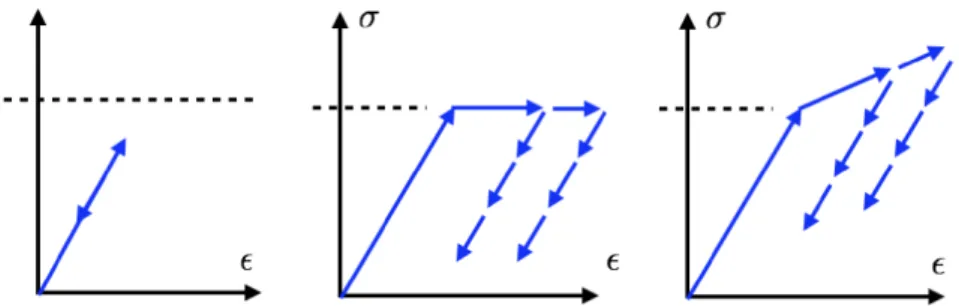
Figure 17. Elastic behavior (left), elastic–perfectly plastic behavior (center), and
elastoplas-ticity with linear hardening (right).
embedded data point with its closest neighbors) with respect to every original coordinate at-tached to each embedded data point, one can conclude that correlations exist between the ini-tial and reduced coordinates (color grading or low statistical variance). When the dispersion in-creases to a large extent, one can infer that the initial coordinate analyzed is not directly corre-lated (even if it could be correcorre-lated in a more complex or combined manner) as discussed.
To prove the generality of these conclusions, Section 4 addresses a more complex scenario. It deals with the constitutive modeling of materials, particularly those whose behavior depends on the deformation history of the material.
4. Simple mechanical behaviors
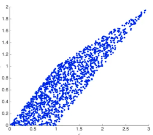
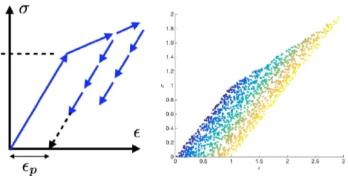
In this section, we consider some simple 1D mechanical behaviors as that depicted in Figure 17. Figure 18 shows a set ofM = 1500 strain–stress pairs yi = {εi,σi}, i = 1,...,M, related to an hypothetical 1D elastic–plastic behavior with linear hardening. The depicted points represent the final mechanical state (strain–stress) ofMloading–unloading random trajectories. It can be noted that with only the information of possible mechanical states, given a strain value, there are many probable values of permissible stresses and vice versa.
There is nothing physically inconsistent in having multivalued fields, but if one is looking for single-valued stress, then an extra latent variable must be introduced.
If, as in Section 3, we apply the k-PCA on the dataset yi, i = 1,...,M, as expected, the 2D manifold appears embedded in theR3space as depicted in Figure 19. This indicates that three mechanical variables, stress and strain completed by a latent extra variable p, are mutually related (e.g.,σ = σ(ε,p)), giving rise to a 2D manifold embedded in R3.
As previously discussed, many latent variables could be certainly considered for obtaining for example a single-valued stress value. Historically, the plastic strainεp, illustrated in Figure 20, was widely considered as a latent variable. Coloring the reduced pointsξi depicted in Figure 19 according to the plastic strain results in the colored manifold shown in Figure 21. This validates the choice of the plastic strain as a latent variable.
5. Toward alternative representations of the mechanical state
An alternative representation of the mechanical state, avoiding the choice of nonevident latent variables, consists in assuming that the stress at time t depends on the whole strain history, that is, onε(τ), τ ≤ t.
When memory effects are neglected, the mechanical state can be described at time t from the strain and stress increments and the present state of stress–strain. That is, ∀ti = i∆t , yi = {εi,σi,∆σi/∆εi}, where∆εi has a given magnitude and two possible signs (positive in loading and negative in unloading).
Figure 18. Strain–stress mechanical states related to elastic–plastic behavior with linear
hardening.
Figure 19. Elastic–plastic manifold embedded in the 3D space.
Different scenarios can be analyzed:
• Linear elastic regime without plastic strain. In this case, as expected, the slow manifold constituted by the reduced states ξi related to the mechanical states yi, depicted in Figure 22, in the 3D space (ξ1,ξ2,ξ3) becomes 1D.
• Nonlinear elastic behavior (with the tangent modulus ET = Eε2) without plastic strain. In this case, the results are similar to those just discussed. In Figure 23, the nonlinear behavior can be noted.
Figure 20. Plastic strain definition (left) and mechanical states yi colored according to the plastic strain (right).
Figure 21. Manifold colored according to the plastic strain.
• Linear elastic regime with nonzero plastic strain (perfect plasticity—no hardening). In the present case, in the mechanical state within the elastic domain, we recover from yi a reduced slow manifold of dimension two as expected, which is depicted in Figure 24. • Linear elastic regime with nonzero plastic strain (perfect plasticity—no hardening) with
activated damage. In the present case, with respect to the previously discussed scenario, we presume that the material degrades with the magnitude of the plastic strain and the tangent modulus decreases accordingly. As Figure 25 depicts, this case is quite similar to the previous scenario. However, when coloring with respect to the tangent modulus, the expected uniform degraded map is noted.
• The present case study considers, in addition to the points inside the elastic domain, another set of mechanical states on the elastic domain boundary with a different
Figure 22. Slow manifold related to linear elastic behavior and colored according to the
tangent modulus (i.e.,∆σi/∆εi).
Figure 23. Slow manifold related to nonlinear elastic behavior and colored according to the
tangent modulus (i.e.,∆σi/∆εi).
instantaneous tangent modulus when loading and unloading. As Figure 26 reveals, the mechanical manifold is now richer with points on the elastic domain boundary separated from the elastic manifold. In the solution depicted in Figure 26, damage is not activated. In the presence of damage, the reduction in elastic tangent modulus scales with the plas-tic strain. The slow manifold is colored according to the tangent modulus as shown in Figure 27.
• The last scenario adds an extra richness to the constitutive behavior. At the mechani-cal states within the elastic domain, the elastic tangent modulus is affected by a latent
Figure 24. Strain–stress points associated with states within the elastic domain with
nonzero plastic strains (left) and the associated slow manifold colored according to the tan-gent modulus (right).
Figure 25. Slow manifold related to damageable elastic–plastic behavior operating within
the elastic domain colored according to the tangent modulus.
variable that is the product of the plastic strain with another extra variable. The latter, which could represent strain-rate sensitivity, is assumed to take arbitrary values here due to the fact that we are more interested in methodological aspects than in physical con-siderations. The considered mechanical states are depicted in Figure 28. When apply-ing the k-PCA to the set of mechanical states yi = {εi,σi,∆σi/∆εi}, the resulting mani-fold remains 3D. As expected, no dimensionality reduction is accomplished as Figure 29 reveals, where many values of the elastic tangent modulus can be found for the same values of the stress and strain. To investigate the nature of this behavior, we depict in Fig-ure 30 the elastic tangent modulus versus the plastic strain, where as expected it can be noted that the former does not depend exclusively on the latter. By applying the k-PCA to the data shown in Figure 30, which are nonseparable in two dimensions, one expects
Figure 26. Slow manifold related to elastic–plastic behavior operating within the elastic
domain and on the elastic domain boundary colored according to the tangent modulus.
Figure 27. Slow manifold related to elastic–plastic behavior operating within the elastic
domain and on the elastic domain boundary, colored according to the tangent modulus, when damage is activated.
to separate them by embedding in a 3D space as previously discussed and as Figure 31 proves. Finally, Figure 32 presents the slow manifold from Figure 31 but now colored with respect to the plastic strain or the extra latent variable.
Figure 28. Mechanical states within the elastic domain, colored according to the tangent
modulus, the last depending on the product of two latent variables, the plastic strain, and another arbitrarily chosen variable.
Figure 29. Slow manifold related to elastic–plastic behavior operating within the elastic
domain, colored according to the tangent modulus, with the last scaling with the product of the plastic strain and an extra latent variable.
Figure 31. Slow manifold related to the data consisting of the elastic tangent modulus and
the plastic strain.
Figure 32. Slow manifold of the elastic tangent modulus colored according to the plastic
strain (left) and the extra latent variable (right).
6. Conclusion
The present work introduced, tested, and discussed issues related to manifold dimensionality with two major purposes: (i) first, when too many measurable variables are employed, manifold learning is able to discard the useless variables; (ii) second and more important, the same technique can be employed for discovering the necessity of employing and then measuring an extra latent variable that is able to recover and ensure single-valued outputs. Both issues were analyzed and discussed in two case studies, one with respect to structural mechanics and the other with respect to path-dependent material constitutive behaviors.
Indeed, the physical interpretation of the discovered latent variable could imply the introduc-tion of other measurable variables. This topic should be deeply analyzed.
The main interest in discovering these manifolds is that for a new accessible mechanical state, the output can be inferred by a simple interpolation from its neighbors on the manifold. The main aim of the present work is the construction and analysis of these manifolds. Future works, currently in progress, will focus on their use in performing data-driven simulations.
Conflicts of interest
Dedication
This manuscript was written with the help of the contributions of all authors. All authors have given approval to the final version of the manuscript.
Acknowledgments
The first, third, and fourth authors are supported by their respective ESI Group research chairs; their support is gratefully acknowledged. The first author is supported by CREATE-ID ESI-ENSAM research chair. The third author is supported by the ESI Group Chair at the University of Zaragoza. The fourth author is supported by CREATE-ID ESI-ENSAM research chair.
Appendix A. From principal component analysis to its kernel-based counterpart
A.1. Principal component analysis
Let us consider a vector y ∈ RDcontaining experimental results or synthetic data from a numeri-cal simulation. These results are often referred to as snapshots. If they are obtained by numerinumeri-cal simulation, they consist of nodal values of the essential variable. Therefore, these variables will be somehow correlated and, notably, there will be a linear transformation W defining the vector
ξ ∈ Rd, with d < D, which contains the still unknown latent variables, such that
y = Wξ. (11)
The D × d transformation matrix W, which satisfies the orthogonality condition WTW = Id, is the main ingredient of the PCA [8].
Assume that there existMdifferent snapshots y1, . . . , yM, which we store in the columns of a D ×M
matrix Y. The associated d ×Mreduced matrixΞ contains the associated vectors ξi, i = 1,...,M. The PCA usually works with centered variables. In other words,
M X i =1 yi= 0, M X i =1 ξi= 0, (12)
implying the necessity of centering data before applying the PCA.
The PCA proceeds by guaranteeing maximal preserved variance and minimal correlation in the latent variable setξ. The latent variables in ξ are therefore uncorrelated, and consequently the covariance matrix ofξ,
Cξξ= E{ΞΞT}, (13)
should be diagonal.
To extract the d uncorrelated latent variables, we proceed from
Cy y= E{YYT} = E{WΞΞTWT} = WE{ΞΞT}WT= WCξξWT. (14) Pre- and post-multiplying by WTand W, respectively, and making use of the fact that WTW = I,
give us
Cξξ= WTCy yW. (15)
The covariance matrix Cy y can then be factorized by applying the singular value decomposi-tion,
where V contains the orthonormal eigenvectors;Λ is a diagonal matrix containing the eigenval-ues sorted in descending order.
Substituting (16) into (15), we arrive at
Cξξ= WTVΛVTW. (17)
This equality holds when the d columns of W are taken to be collinear with d columns of V. We then preserve the eigenvectors associated with the d nonzero eigenvalues,
W = VID×d, (18)
which gives
Cξξ= Id ×DΛID×d. (19)
We therefore conclude that the eigenvalues inΛ represent the variance of the latent variables (diagonal entries of Cξξ).
A.2. Multidimensional scaling
The PCA works with the covariance matrix of the experimental results, YYT. However, the MDS works with the Gram matrix containing scalar products (i.e., S = YTY) [8].
The MDS preserves pairwise scalar products:
S = YTY = ΞTWTWΞ = ΞTΞ. (20)
Computing the eigenvalues of S, we arrive at
S = UΛUT= (UΛ1/2)(Λ1/2UT) = (Λ1/2UT)T(Λ1/2UT), (21)
which in turn gives
Ξ = Id ×MΛ1/2UT. (22)
A.3. Kernel-based principal component analysis
The k-PCA is based on the fact that data not linearly separable in D dimensions could be linearly separated if they are previously projected to a space in Q > D dimensions. However, the true advantage arises from the fact that it is not necessary to write down the analytical expression of that mapping.
The symmetric matrixΦ = ZTZ, with Z containing the snapshots zi∈ RQ, i = 1,...,M, associated with yi ∈ RD, has to be decomposed into eigenvalues and eigenvectors. The procedure for centering data ziis carried out in an implicit way.
The eigenvector decomposition reads as
Φ = UΛUT, (23)
giving rise to
Ξ = Id ×MΛ1/2UT. (24)
The difficulties of operating in a high-dimensional space of dimension, in general, Q À D, and the mapping unavailability are circumvented by introducing the kernel functionalκ (also known as the kernel trick). This allows computing scalar products inRQwhile operating inRDby applying the Mercer theorem. This theorem establishes that ifκ(u,v) (where u ∈ RDand v ∈ RD) is continuous, symmetric, and positive definite, then it defines an inner product in the mapped spaceRQ. Many different kernels exist; some of them are reported in [8].
References
[1] T. Kirchdoerfer, M. Ortiz, “Data-driven computational mechanics”, Comput. Methods Appl. Mech. Eng. 304 (2016), p. 81-101.
[2] M. A. Bessa, R. Bostanabad, Z. Liu, A. Hu, D. W. Apley, C. Brinson, W. Chen, W. K. Liu, “A framework for data-driven analysis of materials under uncertainty: countering the curse of dimensionality”, Comput. Methods Appl. Mech. Eng.
320 (2017), p. 633-667.
[3] Z. Liu, M. Fleming, W. K. Liu, “Microstructural material database for self-consistent clustering analysis of elastoplas-tic strain softening materials”, Comput. Methods Appl. Mech. Eng. 330 (2018), p. 547-577.
[4] D. Gonzalez, F. Chinesta, E. Cueto, “Thermodynamically consistent data-driven computational mechanics”, Contin.
Mech. Thermodyn. 31 (2019), p. 239-253.
[5] R. Ibanez, E. Abisset-Chavanne, J. Aguado, D. Gonzalez, E. Cueto, F. Chinesta, “A manifold learning approach to data-driven computational elasticity and inelasticity”, Arch. Comput. Methods Eng. 25 (2018), no. 1, p. 47-57.
[6] M. Latorre, F. Montans, “What-you-prescribe-is-what-you-get orthotropic hyperelasticity”, Comput. Mech. 53 (2014), no. 6, p. 1279-1298.
[7] P. Ladeveze, D. Neron, P.-W. Gerbaud, “Data-driven computation for history-dependent materials”, C. R. Méc. 347 (2019), no. 11, p. 831-844.
[8] J. A. Lee, M. Verleysen, Nonlinear Dimensionality Reduction, Springer, New York, 2007. [9] L. Maaten, G. Hinton, “Visualizing data using t-SNE”, J. Mach. Learn Res. 9 (2008), p. 2579-2605.
[10] S. T. Roweis, L. K. Saul, “Nonlinear dimensionality reduction by locally linear embedding”, Science 290 (2000), no. 5500, p. 2323-2326.
[11] N. Kambhatla, T. Leen, “Dimension reduction by local principal component analysis”, Neural Comput. 9 (1997), no. 7, p. 1493-1516.
[12] Z. Zhang, H. Zha, “Principal manifolds and nonlinear dimensionality reduction via tangent space alignment”, SIAM
J. Sci. Comput. 26 (2005), no. 1, p. 313-338.
[13] A. Badias, S. Curtit, D. Gonzalez, I. Alfaro, F. Chinesta, E. Cueto, “An augmented reality platform for interactive aerodynamic design and analysis”, Int. J. Numer. Methods Eng. 120 (2019), no. 1, p. 125-138.
[14] D. Gonzalez, J. Aguado, E. Cueto, E. Abisset-Chavanne, F. Chinesta, “kPCA-based parametric solutions within the PGD framework”, Arch. Comput. Methods Eng. 25 (2018), no. 1, p. 69-86.
[15] E. Lopez, D. Gonzalez, J. V. Aguado, E. Abisset-Chavanne, E. Cueto, C. Binetruy, F. Chinesta, “A manifold learning approach for integrated computational materials engineering”, Arch. Comput. Methods Eng. 25 (2018), no. 1, p. 59-68.
[16] E. Lopez, A. Scheuer, E. Abisset-Chavanne, F. Chinesta, “On the effect of phase transition on the manifold dimen-sionality: application to the Ising model”, Math. Mech. Complex Syst. 6 (2018), no. 3, p. 251-265.