Fresnel diffractive imagery arrays : ground-based validation and space applications

(1)

(2)

(3)

we are building it to detect something that we never know that it ever exists’’, Space instrumentation Laurent KOECHLIN

(4)

(5)

Acknowledgements

Through the years in this thesis, this part is one of the hardest writing parts in my thesis. I do not know how to start writing this. I have learnt many things and done many things, but one certain thing that I surely know is all of this would never be possible, without the support and encouragement of a lot of people.

First, I would like to thank my director-supervisor. For Laurent KOECHLIN, I could not find any words to express how grateful I want to thank you. I owe you more than what I have gain during four years in l’observatoire Midi Pyrénés, . I can still remember what you told me when we first talk about space instruments research. It is now on the first page. You have been my professor, my mentor, my colleague, my friend and a never-ending of moral support and encouragement. You have given yourself so much to help me succeed. If I will have to be a supervisor someday, I wish that I could be a half the advisor that you have been to me.

I would also like to thank the rest of my thesis committee for their support. Roger FER-LET and Farrok VAKILI provided me with invaluable advice, comments on my research, and being my rapporter. It is a pleasure to thanks Dr. Christophe Peymirat, who always takes care of me since my study in master for being my president de Jury. I would particularly like also to thank Arnaud Liotard who had taken care of me as my co-supervisor.

I would also like to express my thanks to Ana Ines de Castro, Paul Deba and Denis Serre who are always be a good friends, commentator and colleagues. I particularly show my gratitude to Jean Pierre RIVET, who always be a great host in Nice and for taken care of me and my thesis work.

I would like to thanks everyone in l’observatoire Midi Pyrénés, who always helps me every time that it is needed, particulary Herve Cafantan for giving me advices and my friends in laboratory, who making my life in here feel comfortable.

Here, its all my friends in Toulouse. You make me feel at home and I thank you all for let me enjoy my time here. I have never thought that i will stay here this long. Since I first came to Toulouse, you made me feel comfortable and had a great time.

Finally, I would like to indicate this gratitude to my family, who always understand and support me along this journey.

(6)

(7)

Remerciements

C’est avec mon mal écriture Francaise mais c’est quand même avec mon enthousiasme le plus sincére, respectif et le plus vif que je voudrais rendre mérite á tous ceux qui m’ont aidé á mener cette thése : J’adresse mes plus vifs remerciements ´L mon directeur de thése, Monsieur Laurent KOECHLIN pour avoir accepté de diriger ma thése et pour sa compréhension et son soutien intellectuel et moral ainsi que pour le temps qu’il a consacré aux travaux fastidieux de relecture pendant la période de préparation de cette thése. Je lui suis trés reconnaissant et je le respecte beaucoup pour sa gentillesse, sa grande disponibilité, sa patience, ses conseils courag et et ses altitudes pour travailler en thése et pour ma vie. Ce travaile ne sera pas complete sans lui.

Je tiens aussi á remercier Monsieur le Professeur Christophe PEYMIRAT qui j’ai fait mes études en Master et qui m’a fait l’honneur d’être Président de ce jury. Je tiens également á remercier Monsieur le Professeur Roger FERLET et Monsieur Farroke VALKILI pour avoir accepté d’évaluer mon travail. Je leur adresse toute ma gratitude pour leurs conseils importants et judicieux. Je tiens également á remercier Monsieur Arnaud LIOTARD qu’est ma co-director chez Thales Alenia space.

Je tiens á manifester ma profonde reconnaissance pour la gentillesse que Monsieur Jean-Pierre Rivet m’a accordé pour la correction de ce travail et pour de travail que j’ai fait pendant mes temps en Nice.

Mes remerciements vont aussi á mes amis á l’observatoire Midi Pyrénées. Finalement, je voudrais remercier de tout mon coeur mes parents et mes proches pour leurs encouragements et leur soutien durant mes études en France, sans lesquels je n’aurais pas pu être ici en train d’écrire ces remerciements.

(8)

(9)

A Fresnel Diffractive Imager: Instrument for space mission in the visible and UV 155 B Generation 1.5 testbed of Fresnel Imager : setting up and first images 165 C Generation 2 testbed of Fresnel Imager : first results on the sky 181 D A space Fresnel Imager for Ultra-Violet Astrophysics: example on accretion

disks 199

List of figures 211

List of Tables 211

(12)

(13)

Présentation générale

Un nouveau concept optique est validé dans cette thèse : l’utilisation d’un Imageur Dif-fractif de Fresnel comme instrument spatial. Il est basé sur la focalisation diffractive par anneaux de Soret ("Fresnel zone plate”), et particulièrement adapté pour la haute résolution angulaire et la haute dynamique en astrophysique.

La focalization diffractive a été testée dans notre laboratoire en 2007 [Serre D., 2007] par des mesures optiques. Un premier prototype a été construit en 2006 pour tester la focalisation et différentes fonctions dans le domaine visible : à 600 nm de longueur d’onde. Les résultats ont montré qu’il est possible d’utiliser la focalisation diffractive pour former des images à haute résolution et haute dynamique : 10−6.

La prochaine étape a été réalisée lors de cette thèse par la construction du prototype génération II et par son utilisation sur le ciel. Dans ma thèse, je décris comment on a fait la transition entre les prototypes génération I utilisé dans un laboratoire, et génération II, fait pour l’observation du ciel. Vous pourrez trouver décrits dans la suite : la conception, la réalisation, l’intégration et les résultats des observations.

Pour passer des générations I à II, des modifications ont été faites sur deux parties du prototype : les “module grille primaire” et “module récepteur”. Pour la grille primaire, le nombre de zones de Fresnel est passé de 116 à 696, et le côté a été agrandi de 80 à 200 mm. Sur cette nouvelle grille primaire, nous avons fait des optimisations afin d’obtenir une plus grande dynamique et plus de transmission (luminosité). La dernière version de la grille a moins de barres de maintien (1 sur 3). Des modifications du module récepteur ont aussi été faites pour s’adapter aux nouvelles caractéristiques de la grille primaire.

Les validations sur le ciel de l’imageur du Fresnel ont porté sur deux points : la haute dynamique et la haute résolution angulaire. Les observations ont été faites à l’observatoire de la Côte D’Azur, de juillet 2009 à mars 2010. Les cibles astrophysiques ont été choisies dans ces deux directions : d’une part pour la haute dynamique, avec des écarts de luminosité entre des étoiles proches, graduellement augmentés pour trouver la limite en dynamique ; d’autre part pour la haute résolution angulaire, sur des cibles de plus en plus serrées, la séparation entre les étoiles a été mesurée. Avec des binaires serrées à grand écart de magnitude, on peut tester à la fois la résolution et la dynamique. De telles cibles sont des étoiles doubles comme Sirius AB, ayant 11 magnitudes d’écart en bande I (centrée sur 800 nm), et une séparation de 8” . Nous avons aussi tenté d’imager Procyon AB, qui est un système binaire de séparation 2” avec 12 magnitudes de différence, mais sans succès. Les mesures sur ces cibles ont permis de préciser la limite en résolution angulaire et dynamique.

Un autre type de cibles que nous avons observées sont des objets du système solaire, entre autres Mars et ses satellites. Ils sont difficiles à détecter car ces satellites sont très petits et leurs orbites sont proches du disque étendu et brillant de la planète.

(14)

de l’Imageur du Fresnel. Les résultats obtenus ont permis de savoir comment fonctionne ce type d’instrument dans la réalité en observant directement le ciel, et vont aider à préparer une mission spatiale future.

(15)

Part I

General introduction to Fresnel Imager

concept

(16)

(17)

Chapter 1 Introduction

Fresnel Diffractive Imagery Arrays (FDIAs) belong to a new concept of instruments using a diffractive focusing array. FDIAs has advantages in high resolution and high dynamic range in space observation.(Koechlin L., Serre D., et al, 2005)[10]

To develop Fresnel Diffractive Imagery Arrays for space applications after laboratory conception in 2007 ( Serre D., 2007) [3], ground-based validations are pursued to verify and demonstrate the concepts, performance, characteristics and functions of the instrument for sky observation.

Before it is launched to operate in space, the Fresnel imagery has to be carefully studied and tested in all the aspects that can be tested test on Earth, in order to guarantee the functions and results in space operation. This thesis contains the studies of Fresnel Diffractive Arrays prototype generation II, ground-based validation for sky observation and some parts of this thesis are prepared for future space missions.

In the last part, I will conclude by assessing the result and the performance based on ground-based observation. This will allow us to predict the instrument’s behaviour in space conditions.

I will also describe the modules and the functions that have been studied and prepared for ground validation since the summer of 2009. I describe the conception of optics, propa-gation simulation, integration, optimization and results. This thesis refers and links to other articles of Laurent Koechlin, Denis Serre and Paul Deba. It includes some material from collaborations with CNES and NUVA (Network for ultra-Violet Astronomy).

1.1 Why a Fresnel Imager ?

The Fresnel Diffractive Imager is an instrument with a new focussing concept for future space observation. Since Fresnel diffractive arrays are made of thin foil, this quasi-weightless focussing instrument can be built in meters large dimensions. The larger aperture means the better angular resolution, and more deep sky objects. Therefore, Fresnel imager is proposed as an alternative for future space observation missions.

This concept of diffractive focussing has been applied in optics; but diffractive focussing with arrays for space application is a new concept. Then, this is a pioneer for the next generation of diffractive focussing instruments.

(18)

1.1.1 How it helps science

This thesis presents some of the first results of a Fresnel diffractive array Imager for astro-physics. It demonstrates the conditions and functions of the instrument for sky observation.

With larger size of arrays up to 20-m in UV or 30-meter in the visible, it can resolve deep sky objects at respectively 1.5 to 3.5 mas resolution, see chapter 6. This is expected to have an impact on discoveries made with direct imaging in space.

1.1.2 How the Fresnel imager compares with other focussing devices

Fresnel Imaging systems can be compared to other telescopes for angular resolution. Our 200 mm aperture Fresnel imager is equal to classical telescopes having the same aperture. However, the weight of 200 mm Fresnel array itself is only a few grams.

Another benefit of Fresnel Imaging system is high dynamic range imaging. The dynamic range has reached 10−_{8 in numerical simulations (no air turbulence). With our prototypes of}

80 mm and 200 mm, it has reached 10−6in laboratory on artificial sources, and 2.5 10−6on the sky.

From the above comparisons, the Fresnel imager can be seen as a lightweight optical instrument which, when it is used at large aperture, will provide a high angular resolution and high dynamic range.

1.1.3 The difficulties encountered, and resolved, in this thesis work

The difficulties that I have encountered concern the character and peculiar behavior of this instrument, and the observation of the astrophysical targets. Since Fresnel imaging involves a new concept of astrophysical instrument: it is the first Fresnel focussing instrument used for such sky observation, many problems have had to be detected, understood, and resolved. Some examples are: the alinements, being given the long focal length of the prototype (18 meters), the residual aberrations (coma) of the chromatic correction blazed Fresnel lens, the underestimated stiffness requirement of the mechanical structure (not only the 18m telescope tube, but also the 2m optical rail of the receptor module).

1.2 Principle of light focalisation

Focalisation converts incoming light from a plane wave to a focal point. It is required to con-struct images. Focalisation of light usually means refraction by an optical lens or reflection by a concave mirror.

1.2.1 Principle of refraction

Focalization by refraction is a classical method using an optical element, such as a lens, to focus light onto a focal plane. Light travels as a plane wave before reaching the medium. The curved surface refracts light into a convergent wavefront. Figure 1.1 shows the wavefront travelling through an optical lens and converging to a focal point. (Perez J. P., 2004)[14] Refraction is used in many imaging systems.

(19)

Figure 1.1:Focalization by refraction on a curved surface optics changes a plane wave into a spherical wave to form an image at the focal point.

1.2.2 Principle of diffraction.

Diffraction in light waves was discovered by Huygen in 1678 and developed further by Au-gusten Fresnel in 1829. Diffraction occurs when light wave is limited in cross-section by a diaphragm.

Diffraction patterns are controlled by the dimensions and the shape of the aperture. For example, the diffraction pattern of a circular aperture is shown in figure 1.3 and that of a rectangular aperture is shown in figure 1.4. Figure 1.2 describes the basic experiment where diffracted waves are created by a double slits aperture. In all the above cases, the amplitude of the light wave is added in in-phase positions and cancelled out in out-phase positions. (Perez J. P., 2004)[14]

1.3 Fresnel diffractive focalisation

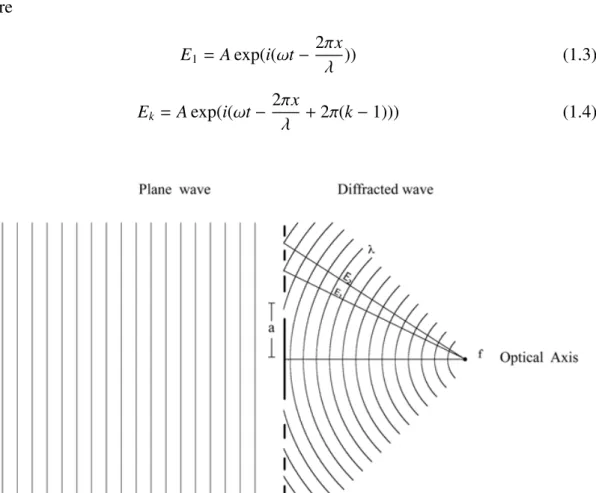
In the Fresnel Imager arrays, diffraction is used to focus light. When light propagates from a distant source through Fresnel arrays, it passes through the open parts of a given Fresnel arrays zone and diffracts, but it is blocked by the opaque parts of the same zone. Figure 1.5 shows how light travels through the open parts of a Fresnel zone and then to focal point. The electric field (amplitude) in a light wave can be described as

E = A exp(iωt − kx) (1.1) while k = 2π/λ

From figure 1.5, we define the wave emerging from the opened part of the first zone as E1, and E2 from the second zone and etc. Thus there is an optical path difference of

λ between two different apertures in consecutive zones. An optical path difference of λ corresponds to phase shift of 2π. The phase shift allows diffracted light to be coherently added at the focal point. The total electric field at the focal point is a sum of diffracted wave from each Fresnel zones. Thus, we can rewrite the output wave as

Ef =

X

(20)

Figure 1.2:

Diffraction of wave by a double slit: first experiment by Thomas Young in the early 1800s. The red nodes and lines represent amplitude of in-phase position from a secondary wavelet and the blank blue anti-nodes represent the out-phase position, where the waves cancel each other out.

Figure 1.3: Diffraction pattern from a circular aper-ture

Figure 1.4: Diffraction pattern from a rectangular aperture.

(21)

where E₁= A exp(i(ωt − 2πx λ )) (1.3) Ek = A exp(i(ωt − 2πx λ +2π(k − 1))) (1.4)

Figure 1.5: A plane wave propagates through the apertures in Fresnel zones. The optical paths (E1and E2)

difference between two Fresnel zones is λ. The diffracted light by arrays aperture converges to a focal point ( f )

This concept has been applied since 1875 as a Soret or Fresnel zone plate (FZP)( Soret J. L., 1875)[22]. It is used in the optical domain as a focusing device, which is shown in fig 1.6. Today, FZP is used in a number of applications such as antenna design for millimetre waves ( Minin I.V. and Minin I.O., 2000)[12].

In classic implementation, a Fresnel zone plate in optics is built the following way: its opaque regions are made from dark material covering the surface of transparent supports. This means drawing the Fresnel zones on the optical surface according to the position of Fresnel zones. The following relation yields to the Fresnel zone radii (a).

a2+ f2= ( f + kλ)2 (1.5) a2 = 2kλ f + (kλ)2 (1.6) where a is the distance of a Fresnel zone from the associated optical axis to determine the radius "a" of the Frensel zone index k in the array.

if kλ f , then we can write equation 1.6 as

(22)

where

f = focal length

k = Fresnel index zone λ = wavelength

From eq.1.7, we have two associated parameters; central wavelength and focal distance, which allows us to determine Fresnel zones radii on the FZP.

1.4 Fresnel array design

Figure 1.6:Circular geometry form of array (original Fresnel Zone Plate in 1875)(Soret, 1875)[22].

Figure 1.7: Orthogonal geometry form of arrays, by Laurent Koechlin et al., developing Fresnel array in orthogonal geometric form from Soret’s Fresnel zone plate in 2005.

The concept of Fresnel arrays , developed by Laurent Koechlin, Denis Serre and Paul Duchon in 2005, is a transformation of Fresnel zone plates from circular geometry to an orthogonal geometry.(Koechlin L. Serre D., Duchon P.)[10]

The orthogonal geometry in Fresnel arrays design supports a rigid mechanical structure of array and reinforces it. Another advantage, which is most useful in space, is the use of void subapertures. This void aperture layout in geometrical arrays is made by using orthogonal bars to maintain Fresnel zones structure and to define the opened aperture at the same time. As a result, there is no optical material in transparent zones.

In space applications, this void subaperture will permit light to pass through the Fresnel arrays , diffract and converge to a focal point without being affected spectrally nor by phase aberration. These advantages mean less weight and a lower cost in building large apertures for space-borne observations in the future.

Fresnel arrays are described by a transmission function having "1" or "0" value respec-tively for a void aperture and opaque area. Equation 1.8 is a transmission function of a Fresnel array as a function of a: the position of the optical axis at the center.

(23)

g(a)= 1 if pa2+ f2 _{∈ [(k}+ f mλ + 14)mλ; (k+ f mλ + 34)mλ [ g(a)= 0 otherwise h(a)= 1 − g(a) (1.8) where

f = focal distance of Fresnel array k = Fresnel zones index

λ = central wavelength

m = diffraction order; in this case, m = 1

To transform the circular Fresnel zone plate into orthogonal form, a transmission law T(x, y) of 2D arrays has been developed from g and h functions as :

Tc(x, y) = h(x)g(y)+ g(x)h(y)

To(x, y) = h(x)h(y)+ g(x)g(y)

(1.9) where x and y are orthogonal;

Tcand Toyield similar arrays in phase opposition (Koechlin L. Serre D., Duchon P.)[10].

One can choose one of these functions to determine the opaque and void areas on Fresnel arrays. We use diffraction at order one, which means that we use the wave front that is obtained by a wavelength shift from a given zone to the next. Figure 1.6 and 1.7 shows the circular and orthogonal geometries.

1.5 Fresnel Imaging System

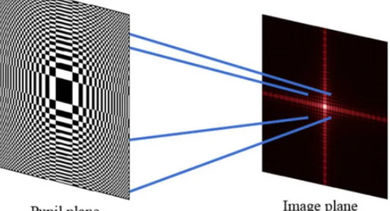
Fresnel Imaging System (FIS) is the actual implementation of the concept either in space or as a ground-based prototype. It is different to other classical Image Systems since it uses diffractive focussing, which is created by thousands of subapertures. An orthogonal geometry array creates a highly confined central lobe in the Point-Spread-Function (PSF): there are a central lobe and four spikes see in figure 1.8. The spikes limit four quadrants in the image field, in which there is a very low background level.

Figure 1.8 shows the circular and orthogonal comparative design. The orthogonal and circular geometry have the same opaque and void parts with respect to Fresnel zone index.

1.5.1 Fresnel Modules

The Fresnel Imaging System (FIS) is the addition of two main modules that are required to perform the vital tasks of collecting light, focusing light, correcting chromatism and con-structing images. The two main modules are classified as : Fresnel arrays module or Primary module, and Fresnel receptor module or secondary module shown in figure 1.9.

(24)

Figure 1.8: Left : circular-othogonal comparative designs, Right : The image given from a point source, Point-Spread-Function (PSF)

(25)

Fresnel Primary module.

The primary module contains the Fresnel array and acts as a diffractor. It focuses light onto the receptor module. The primary module is defined by parameters such as dimension, number of zones and pattern of Fresnel array, that impose the value of parameters to the secondary module such as its position and internal design.

Fresnel Secondary module

The secondary module or receptor module is a collector and correction module, which is placed at the focal plane; for instance, 18 m downstream in prototype generation II as shown in figure 1.9. The focal plane position, at the distance " f " between the modules, is defined by the chosen observation wavelength and other relevant parameters.

Field optics presented as a Maksutov telescope in figure 1.9, collects light from primary array, which is placed in the image plane: distance " f " from the main aperture plane. Light travelling through field optics is focused onto a pupil plane. The field optics conjugates the main array and the pupil plane.

Order "0" mask is used in order to minimise parasite light from the main array that would come from diffraction orders different from “+1”. A mask is placed on the focal plane of the field optics. This mask will enhance the contrast by blocking the light from order "0" of the primary array, which is a parallel beam focused by the field optics.

Chromatic Correction lens (Blazed Fresnel lens at order -1) reorders diffracted light from order “1” of the main array. This results in the equivalent of an order “0”, which we call “+1, -1”(Serre D., 2007)[3] . The beam is now achromatic but no longer convergent. However, the beam has beem compressed, so small optics can be used downstream.

Doublet lens is placed next to the blazed lens to converge wave order “+ 1, −100 to the final image plane. It has a focal length of 350 mm, that focuses the light and creates the final image onto a detector.

1.6 Optical parameters

This section will introduce parameters that are necessary to determine the Fresnel Imaging system specifications. As a Fresnel Imager system has a wide a range of parameters, some of them must be defined as initial conditions.

1.6.1 Focal length

The focal length ( f ) of the primary array is determinant to position the secondary mod-ule with respect to the primary modmod-ule (Serre D. 2007)[20], (D. Serre, P. Deba, and L. Koechlin)[19]. It can be expressed as follows:

f = C

2

8λkmax

(26)

Figure 1.10:Fresnel image system diagram by Paul Deba, describing the primary module as a Fresnel array container collecting and focusing light to the secondary module for chromatic correction and image formation.

where

C = diameter of the Fresnel array

kmax = total number of zones in the Fresnel array

In the study of prototype generation II, we chose the focal length: 18 m as there is an existent refractor tube to support it. The wavelength of 800nm was selected due to optimal observation conditions at this wavelength. The last parameter, kmaxis limited by the smallest

current engraving technology. As a consequence of these constraints, the square section of the primary modules is set at 200 mm.

1.6.2 Wavelength domain limitation

The wavelength domain is limited by the diameter of the field optics in secondary modules. Wavelength domain is described as∆λ :

∆λ λ =

√ 2D

C (1.11)

Field optics (of diameter D), which is a classical optical system, is placed at the focal plane of primary array in order to receive a focused image.

1.6.3 Angular resolution

The angular resolution R of a Fresnel imager can be high, depending upon wavelength and the size of the main array: it behaves like a classical square aperture of the same size.

R= λ

(27)

With a 200 mm aperture and an 800 nm wavelength, the angular resolution defined in 1.12 equals 0.8 arcsec. In a nominal space mission, we definitely have a larger aperture (meter size), and consequently a higher angular resolution. Other parameters associated with Fresnel optics have been described in other publications. (Serre D., 2007)[21] (Serre D. et al,2007)[18].

(28)

(29)

Chapter 2 Photometry and high dynamic range.

This section will describe how photons behave when they travel from the light source to the final image plane in the Fresnel Imaging system(FIS). We assume that the light emitted from the source follows the black body spectrum. Calculation of light transmission through the instrument is made to assess FIS performances.

In an ideal instrument, light would travel through the optical elements with perfect trans-mission. This means there is no absorption, unwanted reflection, diffusion etc. In a practical optic system, not all photons are transmitted through the device. Physical phenomena such as absorption, diffraction etc., occur in the instruments, due to the medium and imperfect op-tics. Our study on Fresnel photometry will assess the instrument’s limitations, and calculate realistic targets for space as well as ground-based testing. The computed number of photons, which reach the detector to construct the image in a Fresnel system, drives the signal-to-noise ratio that indicates image quality.

2.1 Luminosity and limiting magnitude

To determine the number of photons reaching a detector, it is necessary to know the number of photons coming from the light source, and the global efficiency of the Fresnel optical system.

Terms that will be mentioned in this section are brightness and luminosity. These pa-rameters determine the energy that the source emits towards the observer.

Luminosity is a quantity of energy that an object radiates per unit of time (Watt). For example, the luminosity of the sun is 3.846 × 1026 _{Watt. Assuming a given wavelength,}

luminosity is also related to a number of photons emitted per second. In the following, we will refer to brightness: the power received per unit surface (W/m2). For example, the sun delivers a brightness of 1000 W/m2_{at ground level.}

B= LS 4πd2

s

(2.1) where

B = brightness [W/m2] of an object at distance ds

Ls = luminosity radiating from the object

(30)

The brightness can also be expressed in terms of apparent magnitude: in astrophysical usages, physicists use magnitude to describe the brightness of a star.

ma = −2.5 log B Bv (2.2) where ma = magnitude of stars B = brightness of stars, Bv = brightness of Vega.

For instance, the sun has its magnitude of -27.

We can obtain the relation between energy and brightness using this equation:

Etotal = B × t × S (2.3)

where

t = exposure time, S = aperture area.

2.2 Energy and photons

It is important to understand the concept of energy and how it is treated in optical systems. The brightness arriving at the front-end of an optical system is determined by the distance of the light source and its brightness as stated in equation 2.1. Now, we determine the number of photons that are coming into the system for a given wavelength. From the Plank relation, we have the energy of a photon,Ep:

Ep = hc λ (2.4) where h = Planck’s Constant ; 6.6261 × 10−34_Js c = speed of light; 299792458 m s−1 λ = wavelength

A given waveband contains different λ. Here, to determine the number of photons, we consider a limited bandwidth centered around λ and we make the approximation that λ is constant.

Equation 2.4 can be used to determine the number of photons at a certain wavelength. We can determine the number of photons (Np) by:

Np=

Etotal

Ep

(2.5) The number of photon from equation 2.5 is calculated at the entrance of the instrument.

(31)

2.3 Transmission efficiency of the optical system

This process is meant to assess the efficiency of the optical system. Transmission efficiency will determine the number of photons that reach the image compared to the number which is at the entrance.

Absorption, diffusion etc. reduce the number of photons and cause degradation of signal-to-noise ratio. In a Fresnel diffractive array, the transmission can be expressed in two parts, primary and secondary modules. The rate of transmission depends on the performance of these two modules.

In the primary module, the transmission is related to the designed layout of the Fresnel array. The original Fresnel zone plate splits the incoming light wave into several beams, the different diffraction orders [0, +1, -1, +2, -2...+n, -n]. The void and opaque parts in each zone respectively block or transmit the incoming wave. In figure 2.2, the opaque area on array surface has blocked the light, which would have been in phase in phase opposition at the focal point for order different than zero. The maximum focused light into order "1 " of a Fresnel array is about 10% of transmission efficiency.

In the receptor module, the efficiency of transmission is determined like for classical instruments. The transmission of the receptor module is based on the transmission of each optical element. This means that it is necessary to assess the efficiency of field optics devices, corrective lens, focusing lens and dichroic lens. The total efficiency of transmission of a complete system then can be determined as,

Ttotal = TGP× TFO× TLC × TDL× TDC (2.6)

where

Ttotal = total of transmission

TGP = transmission of primary array

TFO = transmission of field optics

TLC = transmission of chromatism correction lens

TDL = transmission of doublet lens

TDC = transmission of dichroic mirror

This transmission will be compromised in optimization process with adpodization profile for contrast enhancement to determine the best parameter for Fresnel arrays, see chapter 3. The efficiency of light transmission may be smaller than in classical systems of identical aperture, but Fresnel design will allow larger apertures in space than classical systems.

2.3.1 Primary array

The primary array’s efficiency of transmission (TGP) gives the percentage of focused light

onto the primary image plane, compared to the incoming light. Numerical simulation of light propagation through a Fresnel array by Denis Serre (Serre D., 2007)[3] shows that we can achieve 6-8 % transmission. Since the number of photons in FIS is essential for an imaging system, it is carefully studied and deliberately optimised to get the most efficient array transmission. For each of our new design of arrays, we have numerically simulated the percentage of transmission. The TGPhas been improved with new design patterns of primary

(32)

Specifications Field optic Optical Design Maksutov-Cassegrains Mirror 150mm Focal Length 1800 nm Diaphragm 45 mm

Table 2.1:Characteristics of Field optic in Fresnel imagery, The diaphram diameter limits the beam.

2.3.2 Field optics

The field optics is a classical Maksutov telescope designed for sky observation. For Fresnel prototype generation II, it is modified to have a diaphragm of 45 mm as a diameter of the field in the primary focal plane. Efficiency of transmission of field optics (TFO) is the proportion

of light passing through the Maskutov telescope. TFOis 79 %.

2.3.3 Order zero mask

The order zero mask is a 2mm diamter disc. It obturates 0.33 % of the order 1 beam. The resulting transmission is then, 99.7%.

2.3.4 Chromatic correction lens

This chromatic correction lens designed by Denis Serre and Paul Deba D. Serre, P. Deba, and L. Koechlin)[19] corrects the diffracted light passing through by operating at order -1 and reorders the light wave to create order ’+1-1’.

This chromatic lens is theoretically estimated to have TLC = 98 % over the useful wave

band. The transmission rate will decrease as much as the observed wavelength is shifted away from the central wavelength. This lens is not coated against reflection, therefore the transmission efficiency is 94%.

2.3.5 Focusing doublet

To construct an image in the final image plane, a doublet lens is positioned a short distance after the chromatic correction lens. It converges the wave from the chromatic correction lens to the focal point. The doublet lens is custom-made. The transmission efficiency of this doublet lens is about 96 %.

2.3.6 Dichroic plate

The dichroic plate is either transparent or reflective depending on the wavelength. It is used to separate incoming light into two channels at different wavelengths. Like a beam splitter, it dispatches light to the science channel and the navigation channel: each with its own

(33)

detectors. One of those channels will receive near infra-red (λ > 742 nm) and the other channel will be more centered on the visible band (λ < 742 nm).(Koechlin L. et al, 2010)[11] Depending on the science targets, we used one band for science and another for naviga-tion or the opposite, to get the best image. Figure 2.1 shows the bandpass of our dichroic plate. The near infra-red band is represented by the green region, which is raised to 98 % above 742 nm. On reflective side, the blue region represents the visible band, which drops to 2 % above 740 nm.

Figure 2.1: Designed bandpass of dichroic plate, the two channels are separated at 745 nm; the blue line corresponds to the visible channel; the green line corrreponds to the IR Channel. (Designed by Paul Deba.)

2.4 Photometry and exposure time

To predict the number of photons at detector level from the previous section, we have the necessary parameters that determine the efficiency of light transmitted into the system. Now, we determine the number of photons falling on the detector by applying equation 2.5. The number of photons that passes through the Fresnel system can be expressed in terms of transmission as Nd = B × t × S hc/λ × TGP× TFO× TLC × TDL× TDC (2.7) where t = exposure time S = aperture area

If we know the magnitude of a source, by using equation 2.5, we can calculate the ex-pected amount of photons on our detector. Table 2.2 shows the numbers of photons, arriving at detector from different sources. In this calculation, the quantum efficiency of the detector (QE) is assumed to be 60% at a selected waveband.

2.4.1 Exposure times

In astrophysical imaging, we have to know the exposure time required for the targets that we observe. Then, equation 2.7 is applied to calculate the exposure time that yields a sufficient

(34)

Source Initial photons time (s) TGP TFO TLC TDL TDC QE Nd Sun 4.44 × 1019 1 0.06 0.79 0.94 0.96 0.98 0.6 1.1 × 1018 Sirius A 1.56 × 109 1 0.06 0.79 0.94 0.96 0.98 0.6 2.6 × 107 Sirius B 9.8 × 104 1 0.06 0.79 0.94 0.96 0.98 0.6 1.6 × 103 Table 2.2:Compared number of photons detected from two different sources (from catalogue data) for a 0.04

m2_{Fresnel array, assuming a 15% reflective bandwidth centered at 680 nm. source: Washington Double stars}

Catalog, interpolatted between R and I band

number of photons to create a usable image. Therefore, exposure time texp can be rewritten

as: texp = Nd × hc B × S ×λ× 1 TGP× TLO× TLC × TDL× TDC × TQE (2.8) Equation 2.8 is an exposure time calculation as a function of the required number of photons, the wavelength, and the aperture area of the instrument. For instance, for an image of Sirius B captured with the condition Nd = 140, an exposure time of 83 milliseconds is

required, which is the exposure time that we have used to detect Sirius B.

2.5 High dynamic range in Fresnel Imager

One of the main features of a Fresnel Imager is high dynamic range imaging. The designed patterns in a Fresnel array influences a diffraction pattern in images. As explained in chapter 1., diffraction in Fresnel Imager causes a very compact focusing on the central lobe and the four spikes of the point spread function. Therefore, there is less energy scattered into the rest of the image.

The specifications of a Fresnel Array are the keys to diffraction pattern and PSF. The number of Fresnel zones, aperture dimension, apodisation, designed pattern of the arrays etc. are vital parameters leading to the dynamic range. High dynamic range in Fresnel imagery is defined by: ratio of the background level over the central lobe.

2.5.1 Fresnel Arrays and dynamic range

The characteristics of images constructed by a Fresnel array are consequences of the design pattern as shown in chapter 1, i.e. round and rectangular layout of transmission pattern. The original Soret’s zone plate (Soret, 1875)[22] is shown in figure 2.2. It is the original circular geometry used since 1875. When the number of Fresnel zones is high, the diffraction pattern from a point source is almost the same as with a round solid aperture, shown in figure 1.3. Since 2005, it has been remodelled into an orthogonal geometry (square format), which can provide high-contrast images, high-angular resolutions and mechanical cohesion (Koechlin L. et al, 2005)[10].

The Fresnel array, which has been transformed, has a number of sub apertures, the di-mensions of which get narrower down by the border of the array as shown in figure 2.4. In the image of a point source (PSF) figure 2.3, the background level in each quadrants is

(35)

re-Figure 2.2: Soret Fresnel Zone Plate 1875

ferred to as b-region, shown in blue. In an a-region, shown in red, are the background levels sampled that are used for the dynamic range assessment.

The orthogonal layout in figure 1.7 was merged into the circular design of figure 2.2 in order to form the bars as a structure to frame the subapertures. This has been in use since laboratory testing. Figure 2.4 shows such a Fresnel array made in 2006, which was made at 80 × 80 mm. It contains 116 Fresnel zones from center to the corner. The array in figure 2.4, was also modified by applying apodization to improve image contrast. The apodization scheme will be explained in the next chapter.

2.5.2 Numerical simulations on dynamic range, and measurements

The dynamic range of Fresnel Imager is studied to assess the instrument’s capabilities and limitations. Numerical wave propagation and image simulations have been made to measure the relation between the dynamic range of image and parameters in a Fresnel array. This study is made by using different patterns of arrays layout and observing the characteristics of the output images.

In the section above, I explained the high dynamic range in Fresnel array design, see fig. 2.3. In this section, I will show the diffractive image from Fresnel array simulation.

Central lobe of PSF

The central lobe of the PSF is shown in figure 2.5, where low light levels are enhanced. It is compact and rapidly decreases as a function of the distance from the center of the field. The central lobe concentrates 60% of the energy spreading over the image plane at order 1. The rest is mostly in the four spikes.

(36)

Figure 2.3: PSF obtained by numerical simulation. Our new Fresnel Design (Orthogonal transformation) extends the contrast between central lobe and background level in quadrants, as b region. The areas where the contrast is sampled for dynamic range assessment are in the a region.

Figure 2.4: 80 × 80 mm Fresnel Array in orthogonal form by Laurent Koechlin et al in 2006, used for Test-bed in laboratory.

(37)

To determine the contrast level, we measure the intensity of the central lobe, and use the standard deviation in the background (outside the spikes and the lobe), see next section. To measure the image’s properties, we use a 100 × 100 pixel square at the center of the image, which is shown in figure 2.5. In the output of the simulation program, the maximum level in one pixel is normalised to 4 × 109.

Figure 2.5:Central lobe measurement on the image obtained by Fresnel imager simulator for dynamic range determination. (Image contrast has been enhanced to display the faint levels of the PSF)

Spikes, quadrants, background.

The PSF in figure 2.6 presents four spikes spreading out of the central lobe. These four spikes divide the image field into four symmetrical quadrants. By sampling the equivalent size 100 by 100 pixels at a distance of 200 pixels from the central lobe, we measured standard deviation of the background level. As shown in figure 2.6, very little energy is distributed in the four quadrants.

This measurement is used to determine the dynamic range in the PSF as a function of the distance from the central lobe. The intensity in the area covered by the four spikes is strong compared to the background but weak compared to the central lobe, approximately 10−3 in both comparisons. The spikes region is not suitable to high-contrast imaging.

2.5.3 Fresnel diffractive Imagery arrays and High Dynamic Range (HDR)

At this step, we use our measurements to calculate the dynamic range (DR) at different distances from the central lobe. We find the dynamic range by determining the ratio between the standard deviation and the maximum value in the central lobe in the background level:

DR= S td IMax

(38)

Figure 2.6: Background measurement on the same field as the figure 2.5. (Image contrast has been enhanced to display the faint levels of the PSF)

In figure 2.6, we measure a dynamic range of 1.8 ×10−8. This value from a numerical simulation is an upper limit in the raw images that we will use in order to estimate the instrument capability.

(39)

Part II

(40)

(41)

Chapter 3 Optimization for prototype generation II,

ground-based observation

Figure 3.1: " Grand Equatorial"dome in observatoire de la Côte d’Azur, built in 1887.

Since 2005 the Fresnel diffractive imager has been developed and tested at the labo-ratoire d’Astrophysique Toulouse-Tarbes (LATT) at Observatoire Midi Pyre´neés by Lau-rent Koechlin, Paul Deba and Denis Serre. A laboratory test-bed, prototype generation I, was made and the concept was successfully demonstrated in 2007 by Denis Serre(Serre D., 2007)[3]. The results, in generation I, have proven that the concept of Fresnel diffractive focalisation satisfied and fulfilled the requirements at small scale. The promising potential

(42)

of high-angular resolution and dynamic range for space observation drives this concept to further developments. In a new step to convince the astrophysical community, we are now trying a larger-scale test with astrophysical targets. As the concept of Fresnel imagery is de-veloped for space mission at high-angular resolution and high dynamic range, it is difficult and expensive to test a prototype in space. A testing on Earth is more feasible. Hence the idea of ground-based Fresnel for sky-observation. The long focal length of Fresnel arrays is a decisive factor; so we had to find a long focal instrument to hold and control the orientation of the prototype. Fortunately, there is a long tube refractor in " Grand Equatorial" dome, located in Nice, see figure 3.1. In figure 3.2, this 18-meter refractor, built in 1887, is main-tained to be functional for visitors and occasional observations. Our prototype generation II has been modified to operate on this refractor mount. To observe real astrophysical targets and observe the sky in real conditions, Fresnel imager in generation II has been enlarged. The modifications are made to both the Fresnel array and to the receptor modules to improve the performance.

In this chapter, we will present the improvements that we made to Fresnel Imager pro-totype generation II. The first sections will show the modifications of the primary array; in particular the parameters that we optimized and the constraints and difficulties that we en-countered. In the following section, I will describe the essential improvements of receptor modules to illustrate the devices that have been integrated and optimized in prototype gen-eration II. The modifications in the receptor module are in relation to those we made to the Fresnel array module.

Figure 3.2: The 76cm diameter refractor’s tube in the " Grand Equatorial" dome, at the Observatoire de la Côte d’Azur, on which prototype generation II will be installed.

3.1 Primary array module

For ground-based observation, an optimization of the primary array is required to improve performance. The 80 × 80-mm array in generation I is not sufficient to collect the light from

(43)

Specifications Prototype generation II Prototype generation I Wavelength 800 nm 600 nm Bandpass 640- 960 nm 480 - 800 nm Focal distance 17.96 m 22.99 m Array size 200 mm 80 mm Fresnel zones 696 Zones 116 Zones Resolution (arcsec) 0.8 1.5 Field Optic diameter 45 mm 35 mm

Number of

sub-apertures 241,860 26,680 Table 3.1: Prototype I & II specifications compared.

astrophysical sources, therefore, the first improvement is building up a larger array. As I explained previously, the first difficulty in ground-based prototype is focal length. The long focal refractor, shown in figure 3.2, is used as a support to manoeuvre both Fresnel Imager modules. Therefore, focal length is limited by the 19-meter tube. The next parameter in this prototype is wavelength adapted to the conditions of sky observation. The last parameter is the minimum diameter of subapertures that the manufacturer can provide. This manufacture constrains our Fresnel zone number, see equation 1.11. Based on these constraints, the dimension of the primary array in prototype generation II is enlarged to 200 × 200 mm maximum. This dimension increases the ability to observe: the larger aperture boosts the instrument’s sensitivity and resolution. With the present limit in engraving technology (20 µm laser beam), the maximum number of Fresnel array zones increased to 696, compared to 116 zones in generation I (Serre D., 2007)[3]. This 6-fold improvement, compared to the first generation, should have improved the dynamic range in similar conditions. However; as we observe through atmospheric seeing, the performances are not comparable, but we are still able to reach a dynamic around 10−5. The central wavelength is shifted from 600 nm to 800 nm in order to minimise atmospheric turbulence effects and diffusion by the atmosphere. Others functions such as tip-tilt, new designed arrays and an enlarged Fresnel blazed lens have also upgraded the performance of the instrument. Changing the focal distance from 22.99 to 17.96 m, was imposed by the size of the 19-meter-long telescope tube. Table 3.1 shows the improvements of parameters and features in prototype generation II compared to those in generation I.

3.1.1 Primary array optimizations

To optimize a Fresnel array for sky observations, modifications of Fresnel’s primary array in prototype generation II are made in three main areas.

1. resolution

(44)

3. dynamic range

These optimizations are the most important parts for our demonstration of the Fresnel imager system. There are relevant parameters, concerning array improvement. However, they are constrained by limiting conditions such as available length of the refractor tube, minimum size of the main array’s sub-apertures (20 um) and wavelength used (800 nm).

Resolution

Angular resolution in prototype generation II has improved thanks to the larger aperture of the Fresnel array. It is adapted to resolve interesting astrophysical targets, such as close binary stars and fine detail on planetary surface. With a 2.5 times larger aperture in Fresnel prototype II, the resolution should be 2.5 times better than with prototype generation I. As a matter of fact, that instrument is made to observe in Near Infra-Red (NIR) at 800 nm. The angular resolution went from 1.5 arcsec in prototype generation I to 0.8 arcsec in generation II, see equation 1.12. This two fold improvement in resolution is a trade-off with wavelength, which is our constraint for sky observation with less atmospheric turbulence and diffusion. Transmission efficiency

Transmission efficiency in prototype II is improved as the collector area is 2.52 _{times larger}

than in prototype I. The geometry of the bars that hold the Fresnel Array structure is opti-mized to allow more light to travel to the focal plane. This will lessen the exposure time required to detect a given number of photons, which increases the limiting magnitude by 2.6. Optimization of transmission efficiency is a delicate problem. As explained in chapter 1, the focused Fresnel diffractive light wave is relatively faint, compared to classical optics systems. Only approximatively 7 % of the incoming wave is diffracted into order 1, which is usable to construct an image, althought about 50 % of input light passes through the Fresnel array; this percentage contributes to light in order 0, order 1, order 2 etc. Only order “1” will be focused onto the field optics afterwards. Therefore, transmission efficiency is a critical issue of the Fresnel array, which must be tackled in prototype generation II. As is shown in figure 3.3, the opaque area includes the opaque parts from the Fresnel zone plate and in addition the orthogonal bars. These bars were set to maintain the structure of the array. They also block the light wave that comes into the Fresnel array. Merging orthogonal bars into the Fresnel zone is also a trade-off between transmission and strength of array structure. The efficienciy of transmission will certainly increase if there are thin bars all over a Fresnel array. Nevertheless, this has a limit as it affects the mechanical stiffness of the array. Determining minimum bars to maintain the stiffness of solid structure is a compromise. By numerically simulating image formation, the best compromise we found was to apply one orthogonal bar in every third Fresnel zone and a bar width corresponding to 0.12 × the pseudo period of the local Fresnel zone. [3]

In figure 3.4, the design of the new array has fewer bars than the previous array in figure 3.3. The orthogonal bars are connected to opaque part of every third Fresnel zone. This design may be less stiff than the one in prototype generation I, but it is enough to maintain the solidity of the Fresnel array.

(45)

Figure 3.3:Fresnel Array design, to diffract light in order 1, and to focus the beam. This layout uses a bar at every Fresnel zone to reinforce and hold the structure of the array. This array design is used in the test-bed of prototype generation I.

(46)

Figure 3.4: Fresnel Array layout, used to diffract and focus light order 1, designed to have fewer bars than the original [one bar in every three Fresnel zone improves the PSF].

(47)

Dynamic range

Dynamic range is improved by Fresnel array layout modifications. The layout of the new bars reduces spikes luminosity and background noise. This, combined with the increased number of Fresnel zones, boosts the dynamic range by a large number.

Dynamic range of Fresnel array in prototype generation II is increased as the number of Fresnel zones and aperture is raised. Another key factor to both transmission and dynamic range is apodization profile.

Apodization and Sampling of numerical PSF Apodization is a general method to im-prove dynamic range by removing the “feet” of the PSF and we apply it to a Fresnel diffrac-tive array layout. It will lower the second lobe and reduce the background level in the field. It enhances signal-to noise ratio in certain cases; such as binary star observation. An apodiza-tion funcapodiza-tion is chosen to produce a better dynamic range around the central lobe of the PSF. The proportion of void/opaque area in a given Fresnel zone is reduced when it goes from the center to the edge of the array. This also means that efficiency of transmission will be decreased as it leaves the central zone. Different apodization functions have been tested in order to get the best dynamic curve for Fresnel arrays in generation II. The functions used for apodization can be cos , cos2or prolate. (Serre D., 2007)[3]

The 1D apodization functions can be expressed as: Apodcos(x)= cos[

2x

C acos(a0)] (3.1) Apodcos2(x)= cos[

2x Cacos(

√

a0)]2 (3.2)

The total transmission rate of the main array drops from 5.84 % to 5.72 % when we use cos2 instead of cos although best dynamic range is obtained by cos2 and the lower limit in transmission for an apodization function is 0.11.

The 2D Apodization in orthogonal coordinates can be written as

Apod(x, y)= Apodx(x)Apody(y) (3.3)

By applying equation 3.3 to the orthogonal function of the Fresnel array, Tc, the modified

transmission is expressed as

Tap(x, y)= Tc(x, y)Apod(x, y) (3.4)

Applying this appodization to modulate the width of the transmission zone, we obtain Fresnel arrays shown in figures 3.3 and 3.4. As you can see, the apodisation function does not go down to zero at the edge of aperture. It stops at a0 = 0.1 since we cannot cut an

aperture smaller than the laser beam, used in the machine tool, 20 µm-laser.

Dynamic range measurement In order to assess the dynamic range of the Fresnel array, we numerically simulate the wave propagation from the Fresnel array to the first focal plane. Our simulation calculates the PSF at given initial conditions such as wavelength, Fresnel array structure, dimension, focal plane position etc. By measuring the simulated output image, we calculate the dynamic range as explained in chapter 2. We tested different designs

(48)

and optimized parameters in order to compare and find the highest dynamic range from this optimisation. The contribution of apodization is shown in figures 3.5 - 3.8. The PSF profile curves shown are a comparison of dynamic ranges with different profiles.

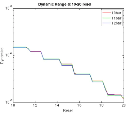
The apodization, which is obtained by modulating the width of each Fresnel zone, is optimized to increase transmission and decrease disturbance to the PSF. The PSF profiles, presented in red, green and blue, are tested to find the best dynamic range within 50 resels of the center of the field. The red curve, issued from a 10% edge transmission apodization, is the finest and gives the largest dynamic range at 5 resels: 10−5_{. The dynamic range can}

drop quicker within 10 resels around the central lobe, but they perform very identically at a distance of 10-20 resels. With a 200 by 200 mm Fresnel array, we chose a0 = 0.11

( transmission at the edge of the array, as a0 = 0.1 would require to engrave minimum

apertures sizes smaller than 20 µm, which the manufacturer cannot provide. The width of the holding bars correspond to 6% of the Fresnel zone to which they are tangent.

Figure 3.5: Dynamic range for 5 resels from the central lobe of the PSF: the red curve corresponds to an edge apodisation ratio of 0.10, green to 0.11 and blue to 0.12.

The results of different apodizations functions are shown in figures 3.5 - 3.6 and figure 3.10. These dynamic range curves correspond to sampled resels in the diagonal from the center of the image, showing the proportion of local intensity to maximum intensity at the central lobe. The best dynamic range measurements in the PSF are shown in figure 3.8. It plots the contrast from the center towards the edge of the image for a length of 50 resels [1₈ of the field].

The relative bar width at 6% of its corresponding Fresnel zone gives the highest trans-mission rate for the array. The apodization improves the dynamic range although it reduces the transmission rate in Fresnel array.

(49)

Figure 3.6:Dynamic range studies for 10 resels from the central lobe of the PSF: the red curve corresponds to an edge apodisation ratio of 0.10, green to 0.11 and blue to 0.12.

Figure 3.7:Fresnel dynamic range from 10 to 20 resels in the diagonal direction from the central lobe of the PSF.

(50)

Figure 3.8: f

or three different a0values, 0.1, 0.11, 0.12 and orthogonal bars tangent to everyzone.Dynamic range for 50 resels from the central lobe of the PSF for three different a0values, 0.1, 0.11, 0.12 and orthogonal

(51)

3.1.2 Primary array fabrication.

The result of the optimization process is a list of specifications used to make a Fresnel array in prototype generation II. This array is to test on sky observation for validation. The results from validation will be used to modify the next version of the Fresnel array. At present, the parameters, which give the best performance in dynamic range and transmission are shown in table 3.2.

Finally, we obtain the parameters that give us the best performance regarding transmis-sion and dynamic range compromise. After this procedure was completed, we sent the array parameters for construction. Once carved, it is used in Fresnel prototype generation II.

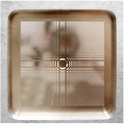
Figure 3.9:Fresnel Array in Generation II prototype, this array is 20 by 20 cm made of a thin metal foil with approximately 250000 apertures. It is held by a mechanical support allowing rotation around its optical axis in order to orient the spikes correctly in the image plane.

Apodisation reduces the size of the sub apertures at the edge of the array. At current technol-ogy level, the cutting machine used for engraving has a 20µm-diameter beam. Therefore the size of the sub apertures has to be larger than 20µm. This limits the apodisation parameter to 0.11, which we use for the current array.

(52)

Figure 3.10:Dynamic range from arrays with different apodization parameters and different bar widths. The last numbers on the middle right of the figure correspond to the overall efficiency into order one(5.67, 6.38). The best curve is the red one at 6% bar width and a0= 0.10. The profile in the bottom is double cosine function.

(53)

Specifications Prototype generation II Array size 200 mm

Array zones 696 Zones Transmission 5.95% dynamic at 10 resel 10−6 dynamic at 20 resel 10−7 dynamic at 50 resel 10−7 Bar width max 0.06 Bar width min 0.06 Apodisation function cos2 Apo Max 0.25 Apo Min 0.11

Table 3.2: Main array’s specifications and performances (From numerical simulation)

(54)

3.2 Receptor Module

The receptor module in prototype generation II is modified to support improved features from the primary array. The receptor module is placed on the image plane of the Fresnel Array 18 meters down stream at the other end of the refractor tube. It is installed on a 2-meter optical rail. Receptor devices in prototype generation II are upgraded to operate in conjunction with the new array specifications. This section will describe the modification and optimization process applied to receptor module.

3.2.1 Field optics

The field optics in prototype generation II still use a Maksutov telescope, the same as that in generation I. This field optics have a nominal focal length of 1800 mm, with a nominal aperture of 150 mm. The modifications made in this generation, to keep up with the new Fresnel array, are a larger diaphragm of the field optic, which increases the linear field at prime focus from 30 to 45mm. Consequently, this 45-mm diaphragm of the field optics also increases the bandpass of focused light into receptor module, as described in chapter 1. The unvignetted bandpass is limited to 690-900 nm.

3.2.2 Order zero mask

The order 0 mask is used to block the light from order 0 that has been focused by the field optics. Its support is modified to let through an enlarged beam (from order “1”). Order “0” mask in prototype generation II has a 2-mm diameter. It is made of a thin opaque disk held by four Kevlar wires. (Koechlin L. et al., 2010)[11] This small mask allows the beam from order “1” to pass around as it has a 40-mm diameter at this position. Figure 3.12 shows the order “0” mask placed inside its tube.

(55)

3.2.3 Chromatic correction lens

In order to correct chromatism in the Fresnel Imaging system, the blazed lens is built to support improvements to the Fresnel array. Since the new Fresnel array has increased the number of Fresnel zones to 696, the chromatic correction lens needed to be modified to serve the additional Fresnel zones. The new blazed lens is made to correct 702 Fresnel zones. It is engraved on a 100-mm fused silica disc and fits a 58-mm diameter beam in the pupil plane.

Figure 3.13:Cell holding the Fresnel correction lens (triangle), and the doublet lens (square PZT actuator).

3.2.4 Doublet lens

The doublet lens and chromatic correction lens are placed in the same box, shown in figure 3.14. This box is baffled to protect those optical elements against dust and stray light. It can be manually tilted and shifted for alignment actions to bust ghosts or other optical de-fects. It is supported by a tip-tilt actuator for atmosphere turbulence compensation. This compensation is required for long-exposure acquisitions.

3.2.5 Dichroic beam splitter

The dichroic beam splitter dividing the beam into two different channels, one for guiding, and one for sciences, has been installed in front of the EMCCD cameras. In figure 3.15, the box contains the dichroic plate and holds the EMCCD cameras. It is baffled to protect against interference from external light.

3.2.6 Detectors

Module detectors are EMCCD cameras, from Andor. The detectors are installed on the same box as a dichroic beam splitter as shown in figure 3.15. One of the detectors is used

(56)

Figure 3.14:Baffled box containing the doublet lens, held by the tip-tilt actuator and the chromatics correc-tion Fresnel lens.

(57)

Figure 3.15: baffeld box containing the dichroic beam splitter, on which the navigation and observation cameras are placed at the final image plane.

for navigation. The other one is used for image acquisition. These channels can be swapped if necessary, depending on the astrophysical targets.

(58)

(59)

Chapter 4 Fresnel diffractive imager’s

ground-based observation

In the previous chapter, we described how the Fresnel Imager System functions and what key components are part of the prototype generation II. This chapter will be split in two parts. The first part will explain the astrophysical targets, which have been imaged during observation at Observatiore de la Côte d’Azur, in Nice, France. There are several types of targets, such as stars, planets, satellites and nebulae. The second part deals with result images from our observation.

Targets for Fresnel sky observation are chosen to assess and validate the performance of the instrument. Ground-based validation has two important objectives. First, to evaluate the characteristics and operational modes of the Fresnel imaging system in a real situation of sky observation. Second, to assess the quality of astrophysical images observed with a Fresnel diffraction Imager. Observing real astrophysical targets has never been done before with the Fresnel array concept. A picture of the building was made with a classical Fresnel zone plate (holographic lens), but without chromatic correction.(Faklis D. et al, 1989)[5]

This chapter will show the preparation phase for Fresnel observations and the results images from our observations. The first section will describe the categories of targets, how the targets are selected, and what assessments are expected from their observation. The second section of this chapter will show targets’ data and the result images from observation, according to the categories.

4.1 Sky targets for Fresnel Observation

As the Fresnel Imager has advantages in high angular resolution and high dynamic range (Serre D., 2007)[21], our selected targets are based on these two aspects. In this case, we divide our targets into two main categories.

High dynamic ranges The targets in this category are objects, which have several points of interests in the field and large differences in brightness. These differences are chosen sufficiently high to demonstrate the instrument’s capabilities. For example: a binary system, in which one of the stars is much brighter than the other. The difference in brightness between them is a test for the dynamic range of the Fresnel imager. This type of targets are binary

Fresnel diffractive imagery arrays : ground-based validation and space applications

Acknowledgements

Remerciements

Contents

I

General introduction to Fresnel Imager concept

11

II

Prototype generation II

35

Annexes

105

Présentation générale

Part I

General introduction to Fresnel Imager

concept

Chapter 1

Introduction

1.1

Why a Fresnel Imager ?

1.1.1

How it helps science

1.1.2

How the Fresnel imager compares with other focussing devices

1.1.3

The difficulties encountered, and resolved, in this thesis work

1.2

Principle of light focalisation

1.2.1

Principle of refraction

1.2.2

Principle of diffraction.

1.3

Fresnel diffractive focalisation

1.4

Fresnel array design

1.5

Fresnel Imaging System

1.5.1

Fresnel Modules

1.6

Optical parameters

1.6.1

Focal length

1.6.2

Wavelength domain limitation

1.6.3

Angular resolution

Chapter 2

Photometry and high dynamic range.

2.1

Luminosity and limiting magnitude

2.2

Energy and photons

2.3

Transmission efficiency of the optical system

2.3.1

Primary array

2.3.2

Field optics

2.3.3

Order zero mask

2.3.4

Chromatic correction lens

2.3.5

Focusing doublet

2.3.6

Dichroic plate

2.4

Photometry and exposure time

2.4.1

Exposure times

2.5

High dynamic range in Fresnel Imager

2.5.1

Fresnel Arrays and dynamic range

2.5.2

Numerical simulations on dynamic range, and measurements

2.5.3

Fresnel diffractive Imagery arrays and High Dynamic Range (HDR)