Stability Guaranteed and Simulation of Heliostat on Testing-Ground

1_{Abstract—Recently, the heliostat field attracts great} attention by searchers in order to boost the electrical performance and harvest great energy. For efficient use, heliostats are generally installed on open-plated areas. The problem stated in this work consists of how heliostats can benefit on distorted grounds? Accordingly, in this work, the dynamic model of heliostat mechanical structure is developed basing on Lagrange formalism. In addition, the system of the heliostat is realized in virtual reality with a real dimension and a program for calculating the sun position and tracking the sun trajectory is developed. Moreover, to ensure a good tracking of the system in control closed loop the state feedback H

synthesis with pole placement based on LMI constraints is used and basing on the quasi-LPV modelling to guarantee the stability of heliostat on testing-ground. The obtained results averred the robustness of the proposed control strategy. This study can be taken into consideration in the implementation of central power towers on different ground shapes.

Index Terms—Quasi-LPV modeling; robotic; state feedback control; pole placement; LMI constraints; heliostat; central power towers; testing-ground.

I. INTRODUCTION

Renewable energies are renewed rapidly which are enough to be considered inexhaustible on a human ladder of time. Solar energy is a kind of available, non-polluting, free and inexhaustible renewable source. Nowadays, it becomes increasingly used, as an alternative to fossil fuel to satisfy the demand for energy.

The world is experiencing important growth in renewable energies as the solar concentrations technology. However, electricity generation from solar radiation is a directly converted, so solar energy is given that spare so that a technology is necessary to concentrate it in order to obtain exploitable temperatures for power generation. Among these technologies, a tower power which is made up of numerous mirrors concentrate the sun ray towards an absorber located at the top of the tower. The uniformly distributed mirrors are called heliostats. Each heliostat is oriented by a solar tracking system and reflects the sunlight precisely to the absorber. The advantage of the heliostat compared to cylindro-parabolic sensors is that the losses in an ambiance are lower because the exposed surface is limited [1].

Single axis solar tracking systems are less costly and their

Manuscript received 24 April, 2017; accepted 11 July, 2017.

control is easy to implement, but their efficiency is lower than that of dual axis [2]. The latter require appropriate control of the two decoupled movements which are used in concentrating thermal power plants for the orientation of heliostats [3], to increase their efficiency which can reach values of 30 % compared to fixed systems [4], again, a computation method of the six angular parameter with a combination of the tracking angle bias strategy and the error-correction model in the of maximizing heliostat tracking accuracy [5]. There are a variety of open loop and closed loop control systems of two axis solar tracking systems for heliostat as well as for photovoltaic systems. In open loop, the sun position is calculated daily, the monthly and the yearly [6]–[7], or another alternative the maximum power point [8]. By exploiting the computing tools, a Programmable Logic Controller (PLC) is used to control the orientation of the system following the position of the sun [9-10], or a programming method based on a Programmable Integrated Circuit PIC16F877 [11]. Another strategy of intelligent control of a solar tracking system based on four light dependent resistor (LDR) which is the Fuzzy Logic Control (FLC) implemented on PIC4550 with two operating modes the sunny or cloudy day [12]. Moreover, the Predictive Control Algorithms was programmed using Arduino ADK and tested, the percentage harvesting of the PV generation was increased around 21,4 % [13]. The advantage of the open loop includes low cost, insensitivity to changed weather conditions, and cloudy skies. The robustness is a drawback of the open loop. In addition, one of the properties of the closed loop is the robustness of the tracking system opposite of external perturbations. Effectively, there exists a cascade control to improve the precision of tracking system in order to increase the concentration photovoltaic modules [14]. Furthermore, one recovers via the analogue input of the Arduino the LDR sensors voltage to generate the necessary pulse width modulation (PWM) of the motors which re-orient the PV panel in order the sun ray was staying perpendicular [15], the other, the PWM were generated from the errors and their variations treated by FLC controller [16].

The use of robotics in the industry reveals a hidden idea to consider the two-axis solar tracking system as a robot manipulator at two degrees of freedom where modelling and control of robots are well advanced in the automation domain similar to industrial computing [10]. The design of

Stability Guaranteed and Simulation of

Heliostat on Testing-Ground

Fatah Bedaouche

1

_{, Abdelouahab Hassam}

1

_{, Mabrouk Boubezoula}

1

1

_{Intelligent Systems Laboratory, Department of Electronic, Faculty of Technology,}

Ferhat Abbas Sétif University 1,

Algeria

robot manipulators in general, using software tools like MATLAB has become more necessary since it is possible to simulate critical operating conditions.

Theory study on controlling periodic mechanical systems have been the subject of intensive research during the last two decades. However, the tracking with robust control over the entire domain of the nonlinear dynamics is a provocative subject of research.

In the main part of this article, we present a mechanical structure of a heliostat developed by SolidWorks software whose design and control require the computation of certain mathematical models, such as models that express the position of the mirrors as a function of the particular variables of the heliostat axes. Indeed, the control of the latter requires a selection of a suitable control strategy. The remainder of the article is organized as follows. In section two the geometry model of the heliostat. In section three, the development of the dynamic model describing its temporal evolution obtained in the form of two nonlinear second differential equations, as well as its modelling quasi-LPV. In section four, the combination of the state feedback control with pole placement using H under LMI constraints and the computed-torque control guaranteeing the tracking and disturbance rejection. In section five, the set schema, relations developed according to the proposed idea and simulation conditions. In section six, discussion of simulation results and finally some remarks have been concluded.

II. PRELIMINARY

The state feedback with H control of a solar tracking system heliostat whose LPV representation in following:

 



 



 



 



 



 



 

 



 



 



 



 



 



 

 



 



 



 



 



 



 

1 1 1 11 12 2 21 22 , , . x t A t x t B t w t B t u t z t C t x t D t w t D t u t y t C t x t D t w t D t u t               _{  }        (1)

Equation (1) can be written in the state representation the form

 









 

 









 

 









 

 





 







 





 



1 1 1 11 12 2 21 22 , A t B t B t M t C t D t D t C t D t D t                        (2)

where _{x t  }

 

2n _{is the state vector, w t  }

_{ }

r _{is the} disturbance vector, _{u t  }

 

m _{is the control input,}

 

p1

z t   is the controlled output, _{y t }

 

p2 _{is the} output vector,



 

t is the time-varying parameter,

 







n n



_, A



t _{ } 

_

_{ }

_

_{ } 1 t n r, B     B 2



 

t



 n m ,

 





 1  1 t p n, C     _{D 11}



 

_t



_{ }p r1 _,

 







1



12 t p m, D



_{ }  _C2



_

_{ }

_t



_{ }



p n2



_,

 







2



21 t p r,

D



   _D22



_

 

_t



_{ }



p m2



_{are the time} varying matrices written under polytopic system given by

 







1v, 2v, 3v, vN



iN1 i

 

iv,

M



t Co M M M M 

_

_



t M (3)

where _i0 and

_

_iN_1_i1, N 2n the vertex of the polytopic system.

Note that the matrices M M M₁v, ₂v, ₃v,Mv_Nare the vertex of the matrix M .

Problem:To find a state feedback [17]

 



 



 



 



 

1 where N _{i i}, i u t K  t x t K  t  t K   

_

(4)

such as the closed loop (1) ̶ (4) is quadratically stable and satisfies the H performance

 

₂

 

₂,

z t  w t (5)

where  0.

Remark: The search of state feedback

 



 



 

u t K  t x t supposes that we have access to all system states.

III. HELIOSTATTOWER INTESTINGGROUND We present in Fig. 1 a mini tower power plant on testing-ground. Each heliostat is characterized by parameters which are height, position in relation to the tower.

Fig. 1. Heliostat field on testing-ground.

Regardless of their heights relative to the tower, the two heliostats are charged to reflect the solar ray towards the absorber at the top of the tower.

IV. MECHANICAL ANDGEOMETRICDESCRIPTION OF HELIOSTAT

The structure of the heliostat is a simple open chain with two joints with geometric representation Fig. 2 [18].

The system composes two body C and₁ C and two₂ joints J and₁ J (Fig. 2). The body₂ C designates the robot₀ frame. Body C is the one that takes the stand heliostat₂

mirrors. The articulation j connects the body C_j to the body C_j₁.

Fig. 2. Robot manipulator with two degrees of freedom.

The parameters Denavit-Hartenberg obtained after associating a fixed reference for each body are listed in following Table I.

TABLE I. GEOMETRIC PARAMETERS OF HELIOSTAT.

Articulation j j dj j aj

0 → 1 q₁ 0 0 r1

1 → 2 q₂ 0 π 2 0

The orientation and position of the normal vector of punctual coordinates M are defined from the transition matrix calculated with respect to the robot frame:

                                  0 2 1 1 2 1 2 1 2 1 1 2 1 2 2 1 2 1 2

cos cos -sin -cos sin cos cos sin cos cos -sin sin sin cos _,

sin 0 -cos sin

0 0 0 1 M M M M T q q q q q X q q q q q q q X q q q q r X q                (6)

The normal vector orientation of the heliostat with respect to the heliostat frame is given by the column vectors R_N and P following:_N

   

1 2

   

1 2

 

2

cos cos sin cos sin T,

N

R  _ q q q q q _ (7)

   

1 2

   

1 2 1

 

2

cos cos sin cos sin .

N T M M M P X q q X q q r X q  _  _ (8)

V. QUASI-LPV REPRESENTATION OFHELIOSTAT The dynamic model is the relations between the torques applied to the actuators and the positions, speeds, and accelerations joint. The equation of the dynamic model takes the following form

 

 

,

 

,

D q q C q q q G q

     (9)

where _{q q q }, ,_{ }

_

n _{are the position, speed, and acceleration} vectors._{  }n _{is the torque input vector. D q}

_{ }

_{ }n n  _is symmetric and positive definite inertia matrix

 

_, n n

C q q_{ }  _{represents the centrifugal and Coriolis} forces, _{G q}

 

_{ } n1 _{is the vector of gravitational forces.}

The dynamic model calculated by the Lagrange formalism

 

 





 





 

 

2 2 2 1 2 2 1 1 2 2 2 2 2 2 2 1 2 2 2 2 2 2 2 2 1 sin cos 0 0 - sin 2 0 1 - - sin 2 0 2 . cos 0 zz xx yy zz yy y xx y xx G q I I q I q q I I I q q _q q I I q q m gX q               _{   }           _{  }                  _   (10)

Respecting the state vector x and input control u , the model (2) can be written [19]

  



 

-1 -1 0 . - , q q q D q C q q q D q                          (11)

The model (11) is nonlinear and can be presented in the polytopic state equation [20]:

 



1 , N i i i i x  t A x B u  

_

  (12)

   

 

-1 -1 0 , 0 - , 0 , I A D q C q q B D q                             (13) where x q q

 

T, u, _D1

   

_{q C q q, }n n  _and

 

  1 _q n n D    .

The time variant parameters chosen are the angular speeds of the axes of the heliostat q₁ and q₂.

From (13): 4 33 43 31 2 0 0 1 0 0 0 0 1 , 0 0 0 0 0 0 0 0 0 0 , 0 0 A A A B B B        _                               (14) where:











2 2 2



33 2 - sin - Ixx Iyy 2q , A q d   (15)

















2 2 2 43 1 2 - sin 2 2 , xx yy zz I I q A q I   (16) 31 1 , B d  (17) 42 2 1 , zz B I  (18) and

 

2

 

2 2cos 2 2sin 2 . yy xx d I q I q (19)

TABLE II. PHYSICAL PARAMETERS OF HELIOSTAT.

Mass of C_{1 m2} 1129.07475 kg Moment of inertia of C₁ I_zz1 1.7191 kg.m2 Moment of inertia ofC₂ I_xx2 2343.5593 kg.m2 Moment of inertia ofC₂ Iyy2 1600.3720 kg.m2 Moment of inertia ofC_{2 Izz2} 777.7458 kg.m2 Centre of gravity ofC₂ X_G2 0.20275 m

VI. STATEFEEDBACKCONTROL

A. H Synthesis with Pole Placement

In this section, we present the state feedback control with H synthesis and pole placement based on LMI constraints for the augmented system (1) [17].

We consider the problem earlier posed in the introduction as well as the reference trajectory tracking with disturbance rejection. For this, the solution to the problem is the application of the following theorem:

Theorem 1: Problem 1 for the polytopic system (3) is solved with scalar  0 if there are matrices

2 2  0 T n n W W_{   }  _and  2  i n n L _{ }  _satisfying: 2 2 1 1 12 1 11 1 12 11 - 0, -T T T T T T i i i i i T T i A W WA B L L B B WC L D B I D C W D L D I    _{   }              (20)

just solve the LMI and reconstruct the state feedback gain 1_{, 1,...,}

i i i N

K _LW _{ .}

Proof: The H_ norm transfer associated with the closed loop for  0 if and only if there exist a symmetric positive definite matrixW satisfying:

- 0,

-T T

cli cli cli cli

T T cli cli cli cli A W WA B WC B I D C W D I    _             (21) where 2 1 1 12 11 , , , , cli i i cli cli i cl A A B K B B C C D K D D             (22)

and the closed-loop poles are placed in the region



, , .



S  r Note that having the poles of a system in



, ,



S

 

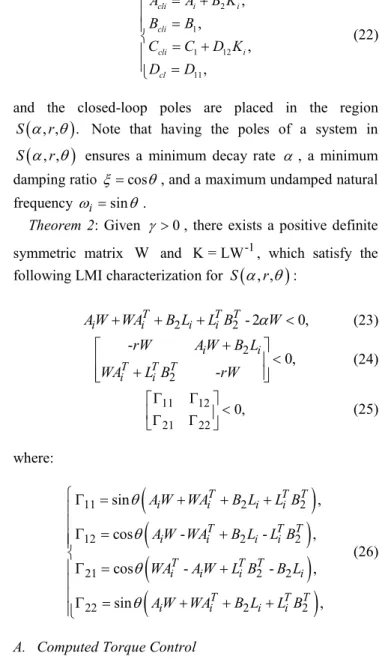
r ensures a minimum decay rate , a minimum damping ratio  cos, and a maximum undamped natural frequency _i sin .

Theorem 2: Given  0, there exists a positive definite symmetric matrix W and K = LW-1, which satisfy the following LMI characterization for S



 

, ,r



:

2 2 - 2 0, T T T i i i i AW WA B L L B



W (23) 2 2 -0, -i i T T T i i rW AW B L WA L B rW            (24) 11 12 21 22 0,      _{ }    (25) where:

















11 2 2 12 2 2 21 2 2 22 2 2 sin , cos - - , cos - - , sin , T T T i i i i T T T i i i i T T T i i i i T T T i i i i AW WA B L L B AW WA B L L B WA AW L B B L AW WA B L L B                           (26)

A. Computed Torque Control

The torque control for the solar tracking of the heliostat can be defined by

 

_d

 

,

 

,

D q q C q q q G q

      (27)

where q_d is the desired acceleration allowing from imposing at the heliostat to track the desired trajectory according to the desired speed.

Consider the following new control law .

d

u q (28)

Then (27) can be rewritten as follows

 

 

,

 

.

D q u C q q q G q

     (29)

VII. METHODOLOGY

A. Sun Position

Sun position is defined by two angles azimuth and elevation expressed by the following relationships [21]:

cos sin

sin ,

cosh

a





(30)

sinh sin sin  cos cos cos ,   (31) where



is the sun declination,  is the solar hour angle and is the latitude of the location.

B. Heliostat Tower Relations

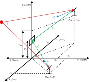
Figure 3 shows the heliostat tower set in a cartesian coordinates system associated with the tower. The position of the heliostat with respect to the tower is defined by that of the frame



X Y Z_{H H}, , _H



, and the coordinates of the target on the tower are given by



0,0,H_T



[22]–[24].

Fig. 3. Cartesian coordinates heliostat-tower and the reflecting of the sun ray by the heliostat to the fixed target.

Coordinated by the centre of the heliostat M are defined by the following expressions:

1 2 1 2 1 2 sin cos - cos cos sin , , . O M H M O M H M O M H M X X X q q Y Y X q q Z Z r X q              (32)

Several useful geometric relations can be obtained in Fig. 2. These relations are important in determining the azimuth  and elevation



of the reflected ray R by the heliostat: 0 0 0 - sin , - cos , , M M M H M X D Y D Z Z H             (33) -1 -tan HT OZM , D _       (34) with 2 2 _. O O M M D X  Y (35)

Substituting (32)–(34) we obtain the following equations

 and



: -1 tan O_O M , M X Y        (36) -1 -tan HT OZM . D        (37)

C. Normal Vector Orientation

The normal vector of the heliostat is defined by the rotation angles azimuth A and elevation H following:

-1 sin cosh cos sin

sin , 2cos cos a H







    _{ }   A (38) -1 sinh sin sin , 2 cos       _{ }   H (39) with









-1

1 cos sinhsin coshcos sin sin cos cos .

2 a a

     (40)

These are the angles to be tracked by the heliostat to move toward desired positions.

D. Heliostat Tower Simulation

The principal objective of this simulation is to reflect the sun ray S by the heliostat towards a fixed target at the top of the tower, and this for different vertical position Z_H between the frame of the tower and the support of the heliostat.

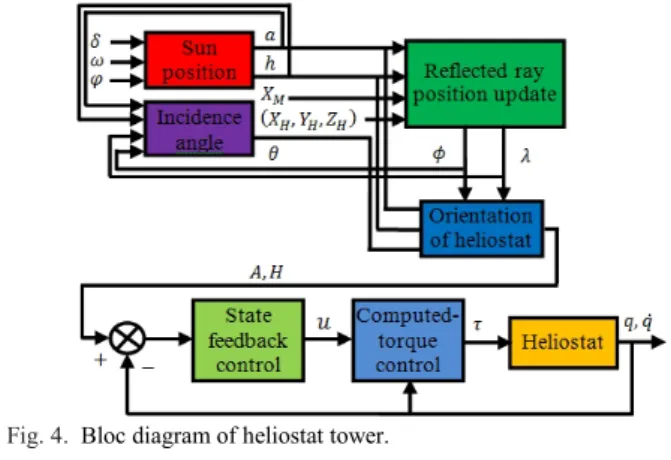
The simulation is realized according to the scheme developed with MATLAB/Simulink presented in Fig. 4, it is different calculation blocks: sun position, sun angle, the reflected ray position and orientation of the heliostat.

Fig. 4. Bloc diagram of heliostat tower.

The heliostat-tower simulation is run for June 21, 2016, using the set of equations (32)–(40). The location of the place and the parameters of the heliostat-tower are collected in the following Table III.

TABLE III. HELIOSTAT TOWER PARAMETERS. Localisation

Latitude



32.380

Heliostat parameters

Height relative to the frame r₁ 1.897 m Center coordinates M of the heliostat X_M (0.316, 0, 0) m

Heliostat coordinates



X Y Z_H, ,_{H H}



(0, 50, ZH) m

Tower parameters

Tower height H_T 10 m

The system matrices (1) and (2) are given by (14) and other matrices as follow:

1 1 1 0 0 1 , , 0 0 0 0 B B B               ₍₄₁₎ 1 2 1 0 0 0 1 0 0 0 0 1 0 0 , , 0 1 0 0 0 0 1 0 0 0 0 1 C C       _{ } _{ }          ₍₄₂₎   11 12 2 21 22 4 2 1 0 , 0 0 0 1 , D D D D    _{ }      (43)

The different gains are obtained with  1,38:

1 2 3 4 -826,810 - 221,570 , 0 - 414,820 -109,28 -808,190 - 219,140 , 0 -391,040 -106,18 -816,080 - 220,170 , 0 - 408,120 -108,47 -831,280 - 222,180 . 0 -379,460 -104,76 K K K K            _{ }  _{  }        _{ }   _{ }            (44)

VIII. RESULTS ANDDISCUSSIONS

The object of the control is to allow to the heliostat to track the imposed trajectory. The gains are adjusted so that the command converges. For this reason, the axes of the heliostat are controlled by a robust state feedback to satisfy the exact requirement of the trajectory tracked.

Figure 5 shows the tracking of the desired position of the normal of the heliostat N in order to reflect the sun rays S towards the fixed target at the atop of the tower with the different vertical position Z of the support of the heliostat_H with respect to the tower.

The position of the heliostat



X ,Y ,Z_{H H H}



from the tower and the height of it are H_T key parameters to calculate the azimuth  and elevation



of the reflected ray R. Figure 6 shows the variation of these two angles



 ,



which are very low, proof that the position of the reflected ray is little variant to say constant, also in both cases the curves are different. Finally, it is true that the height of the support of the heliostat which depends on its mechanical structure influences the response of the tracking system

without affecting its stability because this is guaranteed by the proposed robust control.

(a)

(b) Fig. 5. Heliostat orientation: a)A; b) H.

(a)

(b) Fig. 6. Reflected ray position: a), b)



.

Two cases are observed during the simulation of the heliostat in the testing-ground:

1st case ZH 0 with curve in green colour,

2nd case Z_H 20m with curve in red colour, which we remark that the curves are different.

IX. CONCLUSIONS

This work presents a mechanical structure of a real heliostat realized by SolidWorks software with geometrical representation and dynamic model calculated by the Lagrange formalism. In order to widen the field of application of the heliostat, it is simulated with two different locations and heights in comparison to the tower.

The tracking by reflecting the sun ray towards the fixed target located at the atop of the tower with different heights of the heliostat is the objective of our contribution. Indeed, the robustness of the state feedback control synthesis and pole placement based LMI constraints successfully responds to this objective to have in terms of error tracking on the azimuth and elevation angles of the heliostat the more efficient results.

This study aims for to be an introduction to the integration of the robotics in renewable energies and the installation of tower power plants not only on the level ground but also on the distorted ground.

REFERENCES

[1] Q. Sylvain, Les centrales solaires a concentration. Faculte des sciences appliquees, Universite de Liege, 2007.

[2] S. Abdallah, S. Nijmeh, “Design, construction and operation of one axis sun tracking system with PLC control”, Jordan Journal Applied Science University, pp. 45–53, 2002.

[3] A. J. N. Khalifa, S. S. Al-Mutawalli, “Effect of two-axis sun tracking on the performance of compound parabolic concentrators”, Energy Conversion and Management,vol. 39, no. 10, pp. 1073–1079, 1998. [Online]. Available: http://dx.doi.org/10.1016/S0196-8904(97)10020-6

[4] J. Bione, O. C. Vilela, N. Fraidenraich, “Comparison of the performance of PV water pumping systems driven by fixed, tracking and V-trough generators”, Solar Energy, vol. 76, no. 6, pp. 703–711, 2004. [Online]. Available: http://dx.doi.org/10.1016/j.solener. 2004.01.003

[5] F. Sun, M. Guo, Z. Wang, W. Liang, Z. Xu, Y. Yang, Q. Yu, “Study on the heliostat tracking correction strategies based on an error-correction model”, Solar Energy, vol. 111, pp. 252–263, 2015. [Online]. Available: http://dx.doi.org/10.1016/j.solener.2014.06.016 [6] C. Alexandru, “A novel open-loop tracking strategy for photovoltaic

systems”, The Scientific World Journal, 2013. [Online]. Available: http://dx.doi.org/10.1155/2013/205396

[7] Z. Mi, J. Chen, N. Chen, Y. Bai, R. Fu, H. Liu, “Open-loop solar tracking strategy for high concentrating photovoltaic systems using variable tracking frequency”, Energy Conversion and Management, vol. 117, pp. 142–149, 2016. [Online]. Available: http://dx.doi.org/10.1016/j.enconman.2016.03.009

[8] H. Fathabadi, “Novel high accurate sensorless dual-axis solar tracking system controlled by maximum power point tracking unit of photovoltaic systems”, Applied Energy, vol. 173, pp. 448–459, 2016.

[Online]. Available: http://dx.doi.org/10.1016/j.apenergy.2016.03.109 [9] S. Abdallah, S. Nijmeh, “Two axes sun tracking system with PLC control”, Energy conversion and management, vol. 45, no. 11, pp. 1931–1939, 2004. [Online]. Available: http://dx.doi.org/10.1016/j. enconman.2003.10.007

[10] A. Chaib, M. Kesraoui, E. Kechadi, “Heliostat orientation system using a PLC based robot manipulator”, IEEE 8th Int. Conf. and Exhibition on Ecological Vehicles and Renewable Energies (EVER), 2013. [Online]. Available: http://dx.doi.org/10.1109/EVER.2013. 6521575

[11] S. Abdallah, A. El-Qadan, V. Hamudeh, “Two axes sun tracking system with feedback control on the basis of PIC microcontrollers”, Jordan Journal Applied Science University, Amman 11931 Jordan, 2004.

[12] M. Belkasmi, K. Bouziane, M. Akherraz, T. Sadiki, M. Fakir, M. Elouahabi, “Improved dual-axis tracker using a fuzzy-logic based controller”, 3rd Int. IEEE Renewable and Sustainable Energy Conf. (IRSEC 2015), 2015. [Online]. Available: http://dx.doi.org/ 10.1109/IRSEC.2015.7455104

[13] A. K. Suria, R. M. Idris, “Dual-axis solar tracker based on predictive control algorithms”, IEEE Conf. Energy Conversion (CENCON), Johor Bahru, 2015, pp. 238–243. [Online]. Available: http://dx.doi.org/10.1109/CENCON.2015.7409546

[14] R. Garrido, A. Diaz, “Cascade closed-loop control of solar trackers applied to HCPV systems”, Renewable Energy 97, 2016, pp. 689– 696. [Online]. Available: http://dx.doi.org/10.1016/j.renene. 2016.06.022

[15] T. Kaur, S. Mahajan, S. Verma, Priyanka, J. Gambhir, “Arduino based low cost active dual axis solar tracker”, IEEE 1st Int. Conf. Power Electronics, Intelligent Control and Energy Systems (ICPEICES 2016), Delhi, 2016, pp. 1–5. [Online]. Available: http://dx.doi.org/10.1109/ICPEICES.2016.7853398

[16] A. Zakariah, J. J. Jamian, M. A. M. Yunus, “Dual-axis solar tracking system based on fuzzy logic control and Light Dependent Resistors as feedback path elements”, IEEE Student Conf. Research and Development (SCOReD 2015), Kuala Lumpur, 2015, pp. 139–144. [Online]. Available: http://dx.doi.org/10.1109/SCORED.2015. 7449311

[17] Z. Yu, H. Chen, P. Y. Woo, “Gain scheduled LPV H∞ control based on LMI approach for a robotic manipulator”, Journal of Field Robotics, vol. 19, no. 12, pp. 585–593, 2002. [Online]. Available: http://dx.doi.org/10.1002/rob.10062

[18] W. Khalil, E. Dombre, Modeling, identification and control of robots. Butterworth-Heinemann, 2004.

[19] G. G. Angelis, System analysis, modelling and control with polytopic linear models. Diss. Technische Universiteit Eindhoven, 2001. [20] N. S. D. Arrifano, V. A. Oliveira, “Guaranteed cost fuzzy controllers

for a class of uncertain nonlinear dynamic systems”, Computational & Applied Mathematics, vol. 24, no. 1, pp. 51–63, 2005. [Online]. Available: http://dx.doi.org/10.1590/S1807-03022005000100003 [21] M. Capderou, Atlas solaire de l'Algerie. Office des publications

Universitaires, 1988.

[22] K. K. Chong, M. H. Tan, “Comparison study of two different sun-tracking methods in optical efficiency of heliostat field”, International Journal of Photoenergy, 2012. [Online]. Available: http://dx.doi.org/ 10.1155/2012/908364

[23] A. Gamil, S. I. U. H. Gilani, H. H. Al-kayiem, “Simulation of incident solar power input to fixed target of central receiver system in Malaysia”, IEEE Conf. Sustainable Utilization and Development in Engineering and Technology (CSUDET 2013), 2013. [Online]. Available: http://dx.doi.org/10.1109/CSUDET.2013.6739506 [24] K. K. Chong, M. H. Tan, “Range of motion study for two different

sun-tracking methods in the application of heliostat field”, Solar Energy, vol. 85, no. 9, 2011, pp. 1837–1850. [Online]. Available: http://dx.doi.org/10.1016/j.solener.2011.04.024