A general plasticity and failure criterion for materials of variable porosity

Titre:

Title: A General Plasticity and Failure Criterion for Materials of Variable Porosity Auteurs:

Authors: Michel Aubertin, Li Li, Richard Simon, Bruno Buissière Date: 2003

Type: Rapport / Report Référence:

Citation:

Aubertin, Michel, Li, LI, Simon, Richard et Buissière, Bruno (2003). A General Plasticity and Failure Criterion for Materials of Variable Porosity. Rapport technique. EPM-RT-2003-11

Document en libre accès dans PolyPublie Open Access document in PolyPublie

URL de PolyPublie:

PolyPublie URL: http://publications.polymtl.ca/2620/

Version: Version officielle de l'éditeur / Published version_{Non révisé par les pairs / Unrefereed} Conditions d’utilisation:

Terms of Use: Autre / Other

Document publié chez l’éditeur officiel

Document issued by the official publisher

Maison d’édition:

Publisher: École Polytechnique de Montréal URL officiel:

Official URL: http://publications.polymtl.ca/2620/ Mention légale:

Legal notice: Tous droits réservés / All rights reserved

Ce fichier a été téléchargé à partir de PolyPublie, le dépôt institutionnel de Polytechnique Montréal

This file has been downloaded from PolyPublie, the institutional repository of Polytechnique Montréal

EPM–RT–2003-11

A GENERAL PLASTICITY AND FAILURE CRITERION FOR MATERIALS OF VARIABLE POROSITY

Michel Aubertin, Li Li, Richard Simon, Bruno Bussière Département des génies civil, géologique et des mines

École Polytechnique de Montréal

EPM-RT-2003-11

A GENERAL PLASTICITY AND FAILURE CRITERION FOR MATERIALS

OF VARIABLE POROSITY

Michel AUBERTIN1,3, Li LI1, Richard SIMON1, Bruno BUSSIÈRE2,3

1_{Department of Civil, Geological and Mining Engineering, École Polytechnique de Montréal,} C.P. 6079, Succursale Centre-ville, Québec, H3C 3A7, Canada

2_{Department of Applied Sciences, Université du Québec en Abitibi-Témiscamingue} 445 boulevard de l'Université, Rouyn-Noranda, Québec, J9X 5E4, Canada

3_{Industrial NSERC Polytechnique-UQAT Chair on Environment and Mine Wastes Management} (http://www.polymtl.ca/enviro-geremi/).

2003 Dépôt légal:

Michel Aubertin, Li Li, Bibliothèque nationale du Québec, 2003

Richard Simon et Bruno Bussière Bibliothèque nationale du Canada, 2003 Tous droits réservés

EPM-RT-2003-11

A general plasticity and failure criterion for materials of variable porosity

by Michel AUBERTIN1,3, Li LI1, Richard SIMON1, Bruno BUSSIÈRE2,3

1_{Department of Civil, Geological and Mining Engineering, École Polytechnique de Montréal}

2_{Department of Applied Sciences, Université du Québec en Abitibi-Témiscamingue}

3_{Industrial NSERC Polytechnique-UQAT Chair on Environment and Mine Wastes Management}

Toute reproduction de ce document à des fins d’étude personnelle ou de recherche est autorisée à la condition que la citation ci-dessus y soit mentionnée.

Tout autre usage doit faire l’objet d’une autorisation écrite des auteurs. Les demandes peuvent être adressées directement aux auteurs (consulter le bottin sur le site http://www.polymtl.ca) ou par l’entremise de la Bibliothèque:

École Polytechnique de Montréal

Bibliothèque – Service de fourniture de documents Case postale 6079, Succursale « Centre-Ville » Montréal (Québec)

Canada H3C 3A7

Téléphone: (514)340-4846

Télécopie: (514)340-4026

Courrier électronique: biblio.sfd@polymtl.ca

Pour se procurer une copie de ce rapport, s’adresser à la Bibliothèque de l’École Polytechnique de Montréal. Prix: 25.00$ (sujet à changement sans préavis)

Régler par chèque ou mandat-poste au nom de l’École Polytechnique de Montréal.

Toute commande doit être accompagnée d’un paiement sauf en cas d’entente préalable avec des établissements d’enseignement, des sociétés et des organismes canadiens.

ABSTRACT

Many criteria have been developed to describe the yielding condition, plastic potential, and failure strength of engineering materials such as metal, concrete, rock, soil, and backfill. In this report, the authors first recall some relatively common criteria used to describe yielding and failure of porous materials. It is then shown that the main features of a large number of these criteria can be represented by a unique set of equations. The ensuing multiaxial criterion is applicable to a wide diversity of materials and loading states. A particularity of the proposed criterion, named MSDPu, is that it includes an explicit porosity-dependency. The validity of this general criterion is demonstrated using experimental results obtained on various types of materials.

Key words: criterion, failure, plasticity, porous material, porosity.

RÉSUMÉ

Plusieurs formulations ont été développées pour décrire les conditions d'écoulement, le potentiel plastique et la résistance à la rupture des matériaux utilisés en ingénierie tel les métaux, les bétons, les roches, les sols et les remblais. Dans ce rapport, les auteurs revoient d'abord quelques critères communément utilisés pour définir la limite élastique et la rupture des matériaux poreux. On montre ensuite que les caractéristiques de plusieurs critères existants peuvent être représentées avec un seul système d'équations. Ce critère multiaxial est applicable à une grande variété de matériaux et de conditions de sollicitation. Une particularité du critère proposé, appelé MSDPu, est le fait qu'il inclut une dépendance explicite sur la porosité. La validité de la formulation générale est démontrée en utilisant des résultats expérimentaux obtenus sur plusieurs types de matériaux.

TABLE OF CONTENTS

ABSTRACT ...ii

RÉSUMÉ...ii

TABLE OF CONTENTS ...iii

1. INTRODUCTION ... 1

2. MULTIAXIAL CRITERIA FOR POROUS MATERIAL... 4

2.1 General characteristics ...4

2.2 The development of criteria...6

3. MSDPu CRITERION FOR POROUS MATERIAL... 16

3.1 General description ... 16

3.2 Equations of the MSDPu criterion... 17

3.3 Schematic representation ... 20

3.4 Comparison with other criteria... 25

4. APPLICATION OF THE MSDPu CRITERION... 30

4.1 Identification of MSDPu parameters ... 30

4.2 Graphical representation of experimental results ... 33

4.3 Description and prediction with the MSDPu criterion... 49

5. DISCUSSION………..…….56

5.1 Application to large size rock mass strength ... 56

5.2 Modification of the function Fπ... 56

6. CONCLUSION... 59

ACKNOWLEDGEMENTS ... 59

1. INTRODUCTION

In numerous applications requiring analysis of the mechanical behaviour of engineering materials (metal, concrete, soil, rock, backfill, mining waste, etc.), it is necessary to define the conditions associated with various specific states, including the elastic limit, the initiation of crack propagation, and the peak strength. To describe these particular conditions, engineers generally use mathematical functions, called criteria, expressed in the stress space. Over the years numerous criteria have been proposed to represent the limit of the elastic domain (plasticity criterion), the critical state (corresponding to the critical void ratio when no volume change occurs), the plastic potential (which serves to define inelastic deformation), and the failure strength (associated with the maximum peak stress) and residual strengths. For these and various other states, it is possible to utilise a unified function, where the parameters are defined to represent the distinct phenomena.

Over the years, a large number of criteria have been developed for materials used in engineering. In the last two decades, there has been an abundance of literature published where these criteria have been reviewed, analysed, and compared; the following publications includes such reviews: Yong and Ko (1981), Chen and Saleeb (1982), Desai and Siriwardane (1984), Chen and Baladi (1985), Lubliner (1990), Charlez (1991), Chen and Zhang (1991), François et al. (1991, 1995), Lade (1993, 1997), Skrzypek and Hetnarski (1993), Andreev (1995), Sheorey (1997), Potts and Zdravkovic (1999), di Prisco and Pastor (2000), Desai (2001), and Yu et al. (2003). Some of the better known expressions are summarised later in this report to highlight some of their characteristics. The

and σ3 (the major, intermediate and minor principal stresses, respectively), or a combination of the invariants of the stress tensor σij. One can thus write:

F(σ1, σ2, σ3,) = 0 (1a)

or

F(I1, J21/2, θ) = 0 (1b)

where I1 = tr(σij) represents the first invariant of the stress tensor; J2 = (1/2) Sij Sij is the second invariant of the deviatoric stress tensor Sij (in which Sij = σij – (I1/3)δij; δij = 0 if i ≠ j and δij = 1 if i =

j); and 3 2 1 2 3 3 sin 3 1 J J

θ₌ − 3 _{is the Lode angle which reflects the position of the stress state in the}

octahedral (π) plane (-30° ≤ θ ≤ 30°), in which J3 = (1/3) Sij Sjk Ski is the third invariant of the

deviatoric stress tensor.

Some criteria are based on a single principal stress (σ1 or σ3) or on the two extreme principal stresses (σ1 and σ3). Nevertheless, for general applications, it is usually necessary to use the three principal stresses to adequately represent the behaviour of materials under various regimes of multiaxial loading. Also, when a criterion is expressed from the invariants cited above, it is not uncommon to use only one or two of the invariants; for instance, only J2 is used with the von Mises criterion, while I1 and J2 are included in the Drucker-Prager criterion (see next section). However, a general representation of the behaviour of porous materials should involve the three distinct invariants, including the θ angle proposed by Lode (1926) to provide a better representation of the effect of the intermediate principal stress σ2 (Nayak and Zienkiewicz 1972; Slater 1977).

It can be practical to express the formulation of a three-dimensional criterion, forming a surface in the stress space (σ1 - σ2 - σ3, or σx - σy - σz where the Cartesian axes are the principal axes), with two expressions giving the position and the form of the surface in the I1 - J21/2 plane (function F0) and in the octahedral (π) plane that is perpendicular to the hydrostatic axes σ1 = σ2 = σ3 (function Fπ). One can thus write (Aubertin et al. 1994):

F = J21/2 - F0 Fπ = 0 (2)

2. MULTIAXIAL CRITERIA FOR POROUS MATERIALS

2.1 General characteristics

The behaviour of materials beyond the elastic domain depends on several deformation mechanisms. For crystalline materials with a ductile behaviour (such as metals, ice and certain rocks at high temperature), inelastic straining is generally controlled by dislocations motion, which may cause hardening and sometimes damage due to the creation of voids. For materials exhibiting a brittle behaviour, such as consolidated or cemented materials (rock, concrete, plaster, backfill, etc.), the inelastic deformation is principally due to the initiation and propagation of micro cracks, which may eventually become macroscopic fractures that are often associated with the failure condition (Charlez 1991; Aubertin et al. 1998). With loosely consolidated particulate materials (which is usually the case for most soils, powders, and grains), frictional sliding and crushing generate inelastic deformation (under drained conditions) up to a critical state (iso-volumetric) condition (Lade 1977; Chen and Saleeb 1982; Desai and Siriwardane 1984).

In all cases, material loading results in a transitional behaviour, such as the passage from the elastic regime to the inelastic regime or from the pre-peak phase to the post-peak phase. The condition that define the passage from one phase to another may be included in the constitutive laws describing (or predicting) the material response under specific loads. Such conditions are expressed by mathematical functions called criteria. In the great majority of cases, a criterion is formulated with the stress tensor σij (or its invariants) and it may be shown graphically in the σ1 - σ2 - σ3 space where it takes the form of a three-dimensional surface.

An important impetus behind the development of 3D plasticity criteria was the need for a generalised representation (in the tridimensional stress space), for yielding observed under uniaxial

testing of metals. Criteria used to define the elastic domain are usually expressed by a scalar function of σij. Experience has shown that for most isotropic and homogeneous materials, the elastic

domain (initial and actual) is convex (Halphen and Salençon 1987). This implies that the criterion used to mathematically define this domain should represent a convex surface in stress space.

In elastoplasticity, a plastic potential is generally introduced in the multiaxial flow law to define the manner in which plastic strain evolves. This potential is often mathematically close to the yield criterion (e.g., Desai and Siriwardane 1984). Such potentials are also used in visco-plasticity (Lemaître and Chaboche 1988; Lubliner 1990).

There are also functions used for describing the peak strength (failure criterion), the threshold for crack initiation (damage criterion), the critical state condition (where a constant void ratio is reached), and the residual strength.

The criteria most often used in engineering generally involve few material parameters that are easily obtained by standard laboratory testing, and have a clear physical meaning. A criterion must satisfactorily describe the important characteristics of the observed behaviour. The expression of the criterion should be unique and form a continuous (and convex) surface in stress space. It should also be reducible to the classic criteria (such as von Mises or Coulomb) for particular cases. The expression should also be capable of reproducing the particularities of more elaborate functions developed over the years, based on observations of fundamental materials behaviour. In

geo-1977; Baladi and Rohani 1979; Desai 1980; Michelis and Brown 1986; Novello and Johnston 1995, 1999), as these were based on experimental observations of the behaviour of soils and rocks.

2.2 Development of existing criteria

The development of most plasticity and failure criteria employed by engineers followed two major axes, one used in mechanical metallurgy and the other in geotechnics (for geomaterials).

For metals, it is common to use a criterion that is independent of the first stress invariant, I1 (or of the mean stress σm = I1/3); this is the case with the Tresca (1868) and von Mises (1913) criteria. The frictional component associated with the effect of the spherical (hydrostatic) portion of σij is thus

neglected. In the case of Tresca, the criterion is based on J2 and J3, the second and third invariants of the deviatoric stress. In the case of the (Huber-) Mises criterion, only J2 is considered; it can be

written as J21/2 = σu/√3 (where σu is the uniaxial strength). This last criterion has been judged to be more representative of the general behaviour of metals (Halphen and Salençon 1987).

For the most part, models employed for porous metals and metallic compounds (including metal powders) have kept their roots in the von Mises criterion, or in a version modified by Schleicher (1926) to take into account the difference in strength between uniaxial strength in tension and in compression (e.g., Lee 1988; Lubliner 1990). Furthermore, the von Mises criterion has been extended by Gurson (1977) to describe yielding and the evolution of voids in porous materials; this well known criterion has then given birth to a variety of somewhat similar criteria (e.g., Tvergaard 1981, 1991; Tvergaard and Needleman 1984). There also exist numerous other criteria for porous metals, which can be reduced to the von Mises criterion for particular cases (e.g., Hjelm 1994; Theocaris 1995; Altenbach and Tushtev 2001a, b; Altenbach et al. 2001).

On the other hand, the Coulomb criterion has served as a starting point for the great majority of criteria used for geomaterials (soil, rock, concrete, backfill, etc). In its basic version, the Coulomb criterion (or Mohr-Coulomb criterion) only uses two principal stresses, σ1 and σ3, with two basic material parameters, c (cohesion) and φ (internal friction angle). This criterion is represented by a line in the Mohr plane σ - τ (where σ and τ are the normal and shear stresses on the given plane, respectively), or in the σ1 - σ3 plane. When generalised in three dimensions, the Coulomb criterion is linear in the I1-J21/2 plane and it takes the form of an irregular hexagon in the plane of the octahedral stresses, with the axes of symmetry corresponding to the six summits of the Tresca criterion to which it is closely related in the π plane. Drucker and Prager (1952) proposed a circular version of the Coulomb criterion in the octahedral plane (similar to von Mises criterion), while maintaining the linear relationship between I1 and J21/2 (without a contribution from θ or J3). Zienkiewicz and collaborators (Nayak and Zienkiewicz 1972; Zienkiewicz et al. 1972; Zienkiewicz and Pande 1977) have later proposed a modified version of the Coulomb criterion, represented by a rounded triangle in the π plane, with the major axes oriented at a Lode angle of 30° (θ corresponding to conventional triaxial compression testing, CTC).

Starting with the Coulomb criterion, a more general representation of soils behaviour was proposed with the Cambridge model (Roscoe et al. 1958, 1963; Schofield and Wroth 1968), which in turn inspired numerous other expressions, several of which are identified in Table 1 and in Figure 1. These include the "Cap" type criteria elaborated by Desai and collaborators (e.g., Desai 1980; Desai

Despite these numerous developments, the simplified criterion of Drucker and Prager (1952) continues to be used regularly for numerous frictional materials because of its simplicity (e.g., Bousshine et al. 2001 for soils; Radi et al. 2002 and Liu et al. 2003 for rocks; Hsu et al. 1999 for other porous materials). Nevertheless, it is known that this simplified criterion is not representative of many aspects of porous materials behaviour, considering its linearity in the I1 - J21/2 plane (a well known limitation) and also because it neglects the effect of J3 (or of θ). This latter aspect was again made obvious recently by Peric and Ayari (2002a, b) who demonstrated that the generation of pore pressure during geomaterial loading depends on the Lode angle.

Among the existing multiaxial criteria, some include a dependence on the initial (or actual) porosity of the material. This is the case with the Gurson (1977) model and it’s many variations (e.g., Tvergaard 1981; Tvergaard and Needleman 1984; Ponte-Castaneda and Zaidman 1994; da Silva and Ramesh 1997; Mahnken 1999, 2002; Ragab and Saleh 1999; Khan and Zhang 2000; Li et al. 2000; Perrin and Leblond 2000). It is also the case with those of Shima and Oyane (1976) and Rousselier (1987).

Comparative summaries (with some critical reviews) on various existing criteria have been presented by Chen and Saleeb (1982), Desai and Siriwardane (1984), Lade (1993), Olevsky and Molinari (2000), Mahnken (2002), Yu et al. (2002). Over the last several years, there have been some more general functions developed in a convergent manner to reproduce in a unified framework the characteristics of the main criteria developed for various porous materials (e.g., Haggblad and Oldenburg 1994; Ehlers 1995; Desai 2001; Lewis and Khoei 2001; Mahnken 2002). This is also the case for the criterion proposed in Section 3.

Table 1 presents the core equations of many multiaxial criteria developed and utilised for engineering materials with a frictional (pressure dependent) component (i.e. with an influence of I1). A schematic presentation of the resulting surfaces of these various criteria is shown in Figure 1.

Table 1. Three-dimensional criteria used for frictional porous materials.

___________________________________________________________________________________________________________

Identification Equations and Parameters References

___________________________________________________________________________________________________________ Mises-Schleicher J2 = ((σc−σt)I1+σcσt)/3 Schleicher (1926)

Mohr-Coulomb J2 =((I1/3)sinφ+ccosφ)/

(

cosθ−sinθsinφ/ 3

)

Chen and Saleeb (1982)

c and φ, cohesion and friction angle of material, respectively.

Drucker-Prager J2 =αI1+k Drucker and Prager (1952)

) ( ) ( ) 12 ( ) (σc−σt α +ασcσt σc−σt = / / k _; α=2sinφ/

(

3(3−sinφ)

)

Cam-Clay J₂ =−α_CMI₁ln(I₁/I₁₀) Roscoe et al. (1958, 1963) Cam-Clay modified _{J2= αCM I1}(_I10−I1) Roscoe and Burland (1968) DiMaggio-Sandler fixed surface: f1= J2+γexp(−βI1)−α=0 DiMaggio and Sandler (1971)

"Cap": ( )2 2 2 1 2 2 2 R J I C R b f = + − =

R, ratio between the major axis a and the minor axis b of the ellipse;

α, β, γ, C, material parameters SMP 2 3

(

)

sin3 (3 1)

(

2 1

)

2 (1 9 1 ) 0 3 1 2/I + /k− J /I + / − /k = J

/ θ Matsuoka and Nakai (1974)

k, material parameter Shima-Oyane 3 ( (3 ))2 (1 )5 0 1 1 2 2/ +an 2 I / − −n = J a _M M σ

σ Shima and Oyane (1976)

a1, a2, material parameters Gurson 3 2 cosh( (2 ))

(

1 2

)

0 M 1 2 M 2/ + n I / − +n = J σ σ Gurson (1977) Lade

(

3 27

)

(1 a) 0 3 1 /I − I / p −k= I m _{Lade (1977)}

pa, atmospheric pressure; m and k, material parameters

Ottosen

(

) (

2 c

)

(1 c) 1 0 2 c 2 /σ +λ J /σ −bI /σ − = J a Ottosen (1977)

a and b, constants; λ, function of the Lode angle θ:

(

(1 3)cos ( sin3 )

)

cos 2 1 1 θ λ=k / − −k _{, for 30° ≥ θ ≥ 0°}

(

60 (1 3)cos ( sin3 )

)

cos 1 ₂ 1 θ λ₌k _°− / − k _{, for 0° ≥ θ ≥ -30°} k1 and k2, constants Desai

(

2

)

( )1 2 s 1 1 2 a s 1 1 2 ( ) ( ) 1 sin3 / -m m_{p I I} I I J = −α + +γ + −β θ − Desai (1980)

I1s, interval of axis I1 due to the uniaxial tensile strength;

m, parameter due to the change in phase

(contractive to dilatant); γ and β, material parameters; α, tightening function.

Modified Gurson 3 2 cosh( (2 ))

(

1 ( )2

)

0 1 M 1 2 1 2 M 2/ + qn q I / − + qn = J σ σ Tvergaard (1981, 1990) ( (2 ))

(

1 ( )

)

0 cosh 2 3 2 1 M 1 2 1 2 M 2/ + qn* qI / − + qn* =

J σ σ Tvergaard and Needleman (1984)

q1 and q2, material parameters;

n*, function of the porosity: n* = n pour n ≤ n' ) ( ) )( 1 ( /q1 n' n n' / nC n' ' n * n = + − − − pour n > n'

nC, critical porosity at rupture;

n' (< nC), threshold linked to the closing of the voids

Hoek-Brown ₀ 3 1 ) cos 3 (sin 3 cos 2 2 1 2 c c 1 2 c 2  =    _{− + +} − / s m I J m

J θ σ θ θ σ σ Pan and Hudson (1988)

m and s, parameters Sofronis-McMeeking 1 2 1 2 1 1 2 1 2 1 1 2 ) 1 ( 1 cos 2 + − +       − +                       − − = m m / m m m / _n n m I n mn

J θ Sofronis and McMeeking (1992)

m, material parameters. Ehlers

(

1 2 (3 3) sin3

)

2 2 0 1 1 4 1 2 2 1 2 − / γ θ +αI / +δ I −βI +εI −κ= J m Ehlers (1995)

α, β, δ, ε, γ, κ, and m, material parameters

Crushed Rock Salt 2 ₂cos

(

1 2 ₀ 1 ₁2 9

)

12 ₂12

(

(1 ) (1 )

)

₊1 − − _{+ −} − + = m m / / n / n / I n J θ κΩκ κ Hansen et al. (1998)

(

)

1 2 1 v (1− )− + = /m mm v n m n Ω ; nv = n , for n ≥ nt nv = n, for n < nt

and κ0, κ1, κ2, m and nt, material parameters

Lee-Oung _{(1 )(} ( ) _{(1 ) 0} 4 3 2 1 2 1 2+ I + −n C−T)−I − −n CT= n

J Lee and Oung (2000)

C and T, absolute values of the uniaxial strengths in

compression and in tension of equivalent non-porous material.

_____________________________________________________________________________________________

Notes: I10, value of I1 at the crushing of the material under hydrostatic pressure; I3, third invariant of the stress tensor σij; n, porosity;

σc and σt, uniaxial compressive and tensile strengths, respectively; σM, flow stress of an equivalent non-porous material; αCM, slope of

Figure 1 Schematic representation of the surfaces associated with some of the criteria used for porous

materials (see Table 1); the σx, σy, σz axes represent principal axes.

I1 J2 1/ 2 _{Drucker-Prager} Mises-Schlecher von Mises Drucker-Prager M ises-Schlecher von M ises pour I1 = 0 σx σy σz for I1 = 0 I1 J 2 1/ 2 Mohr-C oulomb Hoek-Brown Hoek-Brown M ohr-C oulomb pour I₁ = 0 σx σy σz for I1 = 0 I1 J2 1/ 2 Cam Clay Cam Clay modifié CSL αCM Cam-Clay Modified Cam-Clay modified Cam-Clay Cam-Clay σx (θ = 30°) θ = -30° θ = 0° σy σz I1 J2 1/

2 _{DiMaggio and SandlerDiMaggio et Sandler}

C ap σx (θ = 30°) θ = -30° θ = 0° σy σz for I1 = 15 MPa I1 J2 1/ 2 Gurson Tvergaard Tvergaard et N eedleman

Tvergaard and Needleman

Gurson σx (θ = 30°) θ = -30° θ = 0° σy σz Tvergaard (1981) Tvergaard et N eedleman (1984)

Tvergaard and Needleman

I1 J 2 1/ 2 Lade SMP σx σy σz

Ottosen I1 J2 1/ 2 σx σy σz Desai I1 J2 1/ 2 Desai σx (θ = 30°) θ = -30° θ = 0° σy σz Lee et Oung I1 J2 1/ 2

Lee and Oung

Lee and Oung 2000 σx (θ = 30°) θ = -30° θ = 0° σy σz Shima et O yane I1 J2 1/ 2

Shima and Oyane

S hima and O yane 1976 σx (θ = 30°) θ = - 30° θ = 0° σy σz I1 J2 1/ 2

Sofronis and McMeeking Hansen et al. Hansen et al. 1998 σx (θ = 30°) θ = -30° θ = 0° σy σz Sofronis and M cMeeking (1992) Ehlers I1 J 2 1/ 2 Ehler (1995) σx (θ = 30°) θ = -30° θ = 0° σy σz

A few observations can be made from Figure 1:

‰ When observed in the I1 - J21/2 plane, a few criteria are linear (like Drucker-Prager and Matsuoka-Nakai), but the majority are curved downward. All the surfaces of existing criteria are closed on the I1 axis in tension (for I1 ≤ 0), except for the criteria from von Mises and Tresa (not shown here).

On the positive I1 axis (compression), some of the surfaces are open (criteria of Schleicher, Drucker–Prager, Hoek-Brown 3D, Matsuoka-Nakai, Ottosen), but many others are closed to reflect possible collapse of the porous matrix under high mean stresses. The models that include a closed portion, referred to as a "Cap", ensue from the work of Roscoe et al. (1958, 1963) for soils and of Gurson (1977) for metals. Other closed criteria on the positive side of I1 include those of DiMaggio and Sandler (1971), Shima and Oyane (1976), Desai (1980, 2001), Tvergaard and Needleman (1984), Ehlers (1995), Hansen et al. (1998), and Lee and Oung (2000).

‰ There are a few criteria, like those of Gurson (1977), Shima and Oyane (1976), Sofronis and McMeeking (1992), and Hansen et al. (1998), that do not distinguish between positive and negative values of I1, as they are symmetric about the J21/2 axis.

‰ The vast majority of existing criteria show a singularity at the intersection point of the minimum value of I1 (J21/2), while few others tend to be rounded near this value (e.g. Mises-Schleicher and modified Cam-Clay).

‰ In the π plane, some models have adopted a circular form, with a deviatoric strength J₂1/2 independent of the Lode angle θ (as with the von Mises criterion). This is the case, for example, with the criteria of Schleicher (1926), Drucker and Prager (1952), Roscoe et al. (1958, 1963;

also Roscoe and Burland 1968), DiMaggio and Sandler (1971), Gurson (1977), and Tvergaard (1981). Other criteria have adopted an asymmetric hexagonal form, such as the Tresca criterion. Examples include the general 3D version of the criteria from Mohr-Coulomb, Hoek-Brown (Pan and Hudson 1988), and Hansen et al. (1998). There are also those that use the form of a rounded triangle, such as proposed by Nayak and Zienkiewicz (1972), and Zienkiewicz et al. (1972); these include Lade and Duncan (1973, 1975), Matsuoka and Nakai (1974), Lade (1977, 1997), Ottosen (1977), Desai (1980), Ehlers (1995) and Jrad et al. (1995).

3. THE MSDPu CRITERION FOR POROUS MATERIALS

3.1 General description

The MSDPu criterion was first elaborated to describe the behaviour of hard rocks and other brittle materials with a low porosity. Its basic characteristics are described in Aubertin et Simon (1996, 1998) and Aubertin et al. (1999). The criterion is represented by a surface in the I1 - J21/2 plane that reduces to the non linear Mises-Schleicher MS criterion at low mean stresses and which tends progressively towards the Drucker-Prager DP (or Coulomb) criterion at higher mean stresses. In the π plane, the surface generally takes the form of a rounded triangle. The rounded MS portion at low I1 can be seen as an embedded tension cut-off in the DP failure surface.

The parameters used to define the position and the form of the surface are easily obtained. They include the uniaxial tensile and compressive strengths, σt and σc, and the friction angle on smooth surfaces φb. For brittle materials at low porosity, such as hard rocks and certain types of plaster and concrete, the MSDPu criterion constitutes a generalised three-dimensional version of the Griffith (1924) criterion as modified by Brace (1960) and McClintock and Walsh (1962). It therefore considers that for such materials, the initiation of the propagation of crack and peak strength are controlled, at high confining stresses (or high values of the mean stress), by friction mobilised between the faces of closed cracks. This criterion has later been extended to the case of porous rocks and rock masses (Aubertin et al. 2000), by adding (among other components) a term which closes the surface on the positive axis of I1 (to form a "Cap").

Complementary work has also permitted the recent development of a relationship between the uniaxial failure strength in compression (σc) and in tension (σt), and the material porosity (Li et Aubertin 2003). Porosity (n) constitutes a simple and practical parameter for defining the main

features of isotropic materials microstructure. For this reason, the porosity is often related to effective properties of materials (such as the elastic moduli E, G and K, the rate of propagation of voids, permeability, electrical resistance, and uniaxial strengths). A detailed review of the relationships that exist between porosity n and various characteristics of porous materials is presented by Chen and Nur (1994). These authors also present various approaches used for introducing particular characteristics associated with porosity (distribution, form, concentration of voids) into constitutive equations.

The results presented by Chen and Nur (1994) reveal the existence of a critical porosity (or transitional void concentration) beyond which certain properties change in a marked manner, because of the non-uniformity in the internal distribution of contact area. This critical porosity nC is generally much less than 100% (or nC < 1). For instance, the uniaxial compressive strength of rocks may become nil when n is greater than 40 to 70%. The existence of a critical porosity nC was also introduced by Tvergaard et Needleman (1984) to describe the behaviour of porous materials. The value of such critical porosity depends on the shape of the pores and surrounding grain, as shown by Logan (1987) and Chen and Nur (1994).

It is useful to introduce the influence of the initial porosity (in relation to the critical porosity) in the formulation of inelastic criteria for engineering materials. This concept is included in the approach below.

F0 =

[

(

)

]

1/2 2 c 1 3 2 2 1 1 2 1 2 _{I −2aI +a −a I −I} α (3)

where α, a1, a2, a3 et Ic are material parameters, defined from basic properties. Parameter α is related to the friction angle φ:

α = ) sin (3 3 2sin φ φ − (4)

For brittle materials of relatively low porosity, φ can be approximated by the residual frictional angle (φ ≅ φr). Parameters a1, a2 are defined as follows:

a1 =       + − −       − ) ( 6 ) / ( 2 2 _{c t} 2 t 2 c t c σ σ α b σ σ σ σ (5) a2 = 1/2 t c t c 2 t c ) 3( ) / (             − + + σ σ α σ σ b σ σ 2 ₍₆₎

where σt and σc are uniaxial strength in tension and in compression. The relationship of Li and Aubertin (2003) is used to describe the uniaxial strength as a function of porosity:

      −       +       − = u0 u0 C u0 C u0 u 2 1 ) 2 ( cos ) 2 ( sin 1 1 2 σ σ n n π σ n n π σ σ n x x (7)

where σu is the uniaxial strength, which may be used for compression (σun = σcn) or tension (σun = σtn). In this equation, nC is the critical porosity for which σun becomes nil, in tension (nC = nCt) and in compression (nC = nCc); parameter σu0 represents the theoretical (extrapolated)

value of σun for n = 0. Finally, x1 and x2 are material properties; 〈 〉 are MacCauley brackets (defined as 〈 x 〉 = (x + |x|)/2).

Parameters a3 and Ic serve to represent the porous materials behaviour under high hydrostatic compression, when the surface (yield, failure) closes on the positive side of I1 (for I1 > Icn). The dependence of these parameters on porosity (i.e. a3n and Icn) is discussed in section 4.1. It is noted that for dense materials (low porosity), Icn is very large so this portion of the criterion disappears (i.e. the surface remains open along the positive I1 axis).

The surface in the octahedral (π) plane, which is perpendicular to the σ1 = σ2 = σ3 axis, is represented by the following function of the Lode angle (Aubertin et al. 1994).

Fπ =

[

]

v θ b b b ) 1.5 (45 )sin (1 2 2 1/2 2         − − + o (8) with v = exp(-v1 I1) (9)

Here v is an exponent which reflects the influence of the hydrostatic pressure on the evolution of the surface in the π plane; v1 is another material parameter. For a shape that does not change with I1, v1 = 0 (or v = 1). Parameter b controls the size of the asymmetric surface, at -30° in the π plane

3.3 Schematical representations

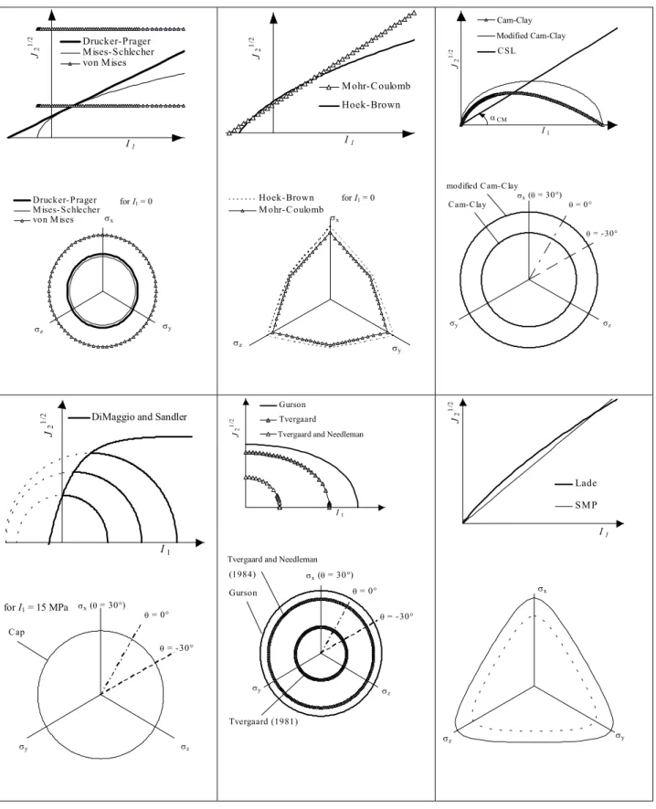
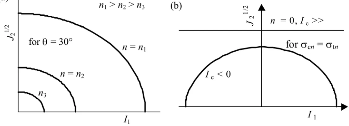
Figure 2 presents schematical views of the MSDPu criterion in the I1 - J21/2 plane (Fig. 2a), in the case of conventional triaxial compression (CTC, θ = 30°), for increasing values of porosity; also shown is the surface in the π plane for a value of v = 1 (Fig. 2b). Figure 2 corresponds to a condition where I1 < Icn. Note on the figure that an increase in porosity (from n1 to n2 to n3) reduces the size of the surface (or the extent of J21/2 for the given values of I1 and θ), because of lower strengths (σcn and σtn) when porosity increases.

Figure 2. Schematic representation of the MSDPu criterion for low porosity materials, with a3n = 0 and ν = 1.

σx (θ = 30°) θ = -30° θ = 0° σy σz n = n1 n = n2 n = n3 I1 = 0 n = n1 n = n2 n = n3 I1 J2 1/ 2 n = n1 n1 > n2 = n3 n = n2 n = n3 θ = 30° J2 1/ 2 n1 < n2 < n3 I1 n = n3 n = n1 n = n2 (a) (b)

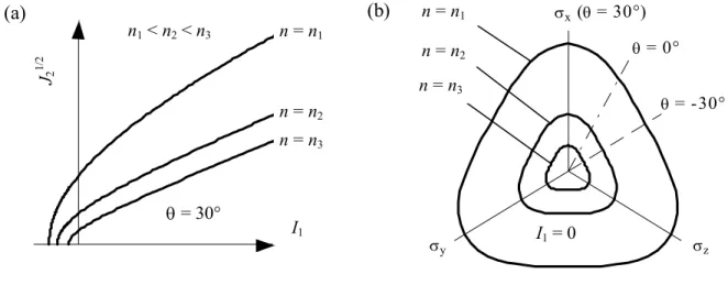
Figure 3 demonstrates the effect of the mean stress I1 on the shape of the surface in the π plane, when v tends towards 0 (or Fπ tends towards 1) at an elevated I1. This situation is associated with a change in the physical mechanisms described by the surface, from a purely frictional behaviour

(Fπ < 1 at θ = -30°) to a ductile/plastic behaviour (at Fπ ≅ 1 at θ = -30°) which may arise in the case of crystalline materials (Aubertin et al. 1994, 1998).

Figure 3. Illustration of the evolution of the MSDPu surface in the π plane, when I1 increases; b = 0.75,

v1 ≠ 0 (v varies with I1). σz (θ = 30°) θ = 0° θ = -30° I1 = 0 σx σy I1 = 10 I1 = 5 pour b = 0.75 I1 = 1.5 v1 ≠ 0

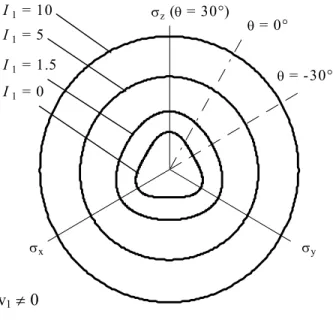
Figure 4 presents a schematical view of the MSDPu surface for a material with a relatively low value of Icn (for I1 exceeding Icn). In this case, the closed portion ("Cap") is apparent in the I1 - J21/2 plane

Figure 4. Schematical view of the MSDPu criterion for porous materials with Ic ≅ 0, a3n ≠ 0, v1 = 0 (v = 1), b = 0.75. I1 J2 1/ 2 n = n1 n1 > n2 = n3 n = n2 n = n3 θ = 30° n = n2 n = n1 n = n3 n1 < n2 < n3 I1 J2 1/ 2 σx (θ = 30°) θ = -30° θ = 0° σy σz n = n1 n = n2 n = n3 I1 = 15 n = n1 n = n2 n = n3

When the frictional component is considered negligible (as in the case of ductile metals), α = 0 (or φ = 0). Equation (3) thus becomes:

2 1 2 c 1 3 t c c 1 2 t t 1 2 c 0 ) ( 3 ) ( ) ( ) ( / n n n n n n n n I /b I _{a I I} F _      − − + − − + = σ σ σ σ σ σ (10)

This version of the criterion resembles a Gurson-Tvergaard surface, as seen on Figure 5 (also refer to Section 3.4). Again, the position of the surface depends on the porosity. For n = 0, a von Mises type of surface is recovered (for σt = σc and Ic >> 0).

Figure 5. Representation of the MSDPu criterion for ductile materials, with a3n ≠ 0, α = 0, v1 = 0 (v = 1). I1 J2 1/ 2 n1 n1 > n2 = n3 n = n2 n = n3 for θ = 30° n1 > n2 > n3 n3 n = n1 n = n2 I1 J2 1/ 2 (a) I1 J2 1/ 2 n = 0, Ic >> Ic < 0 forσ cn = σ t n (b) for σcn = σtn

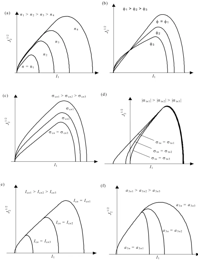
Figure 6 shows the form of the surface in the I1 - J21/2 plane (in CTC) for a consolidated frictional material response. This illustrates the effect of porosity (Fig. 6a), friction angle (Fig. 6b), uniaxial compressive strength (Fig. 6c), and uniaxial tensile strength (Fig. 6d), threshold Icn value (Fig. 6e), and parameter a3n (Fig. 6f).

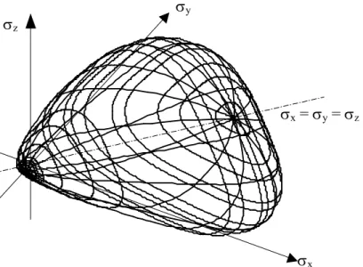
A tri-dimensional view of the complete surface in the σ1 - σ2 - σ3 space is shown on Figure 7 (for the case v = 1 and b = 0.75), for a range of I1 extending beyond Icn.

Figure 6. MSDPu representation in the I1 – J21/2 plane, showing the influence of porosity n (a), angle α (or

φ) (b), uniaxial compressive strength σcn (c), uniaxial tensile strength σtn (d), Icn (e), and a3n (f).

I1 J2 1/ 2 n = n1 n1 > n2 > n3 > n4 n2 n4 n3 (a) _{n1 > n2 > n3 > n4} n = n1 n4 n3 n2 I1 J2 1/ 2 I1 J2 1/ 2 α = α3 α1 > α2 > α3 α = α2 α = α1 (b) J2 1/ 2 I1 φ1 > φ2 > φ3 φ2 φ = φ1 φ3 I1 J2 1/ 2 σc n = σc n 3 σc n = σc n 1 σc n = σc n 2 σc n 1 > σc n 2 > σc n 3 σcn1 > σcn2 > σcn3 σcn1 σcn = σcn 3 σcn2 J2 1/ 2 I1 (c) I1 J2 1/ 2 σt n = σt n 3 σt n = σt n 1 σt n = σt n 2 |σt n 1| > |σt n 2| > |σt n 3| J2 1/ 2 I1 |σtn 1| > |σtn 2| > |σtn 3| σtn = σtn 3 (d ) σtn = σtn 2 σtn = σtn 1 I1 J2 1/ 2 Ic n = Ic n 3 Ic n = Ic n 1 Ic n = Ic n 2 Ic n 1 > Ic n 2 > Ic n 3 (e) J2 1/ 2 I1 Icn 1 > Icn 2 > Icn 3 Icn = Icn 3 Icn = Icn 2 Icn = Icn 1 I1 J2 1/ 2 a3 n = a3 n 3 a3 n = a3 n 1 a3 n = a3 n 2 a3 n 1 > a3 n 2 > a3 n 3 (f) J2 1/ 2 I1 a3 n 1 > a3 n 2 > a3 n 3 a3 n = a3 n 1 a3 n = a3 n 2 a3 n = a3 n3

Figure 7. Schematical representation of the MSDPu criterion in a three-dimensional stress space.

σz

σy

σx

σx = σy = σz

3.4 Comparison with other criteria

The figures shown above indicate that the proposed criterion can take various forms, depending on the values

of the parameters used. It can also be shown that the MSDPu criterion closely reproduces the characteristics

of surfaces associated with other criteria referenced above. Comparisons between MSDPu and some criteria

used for porous materials are shown in Figure 8. In this regard, the proposed criterion may constitute a generalised version of criteria for plasticity and failure developed over the years, for ductile and brittle materials (with variable porosity). Some specific applications of the proposed criterion are presented in the following sections.

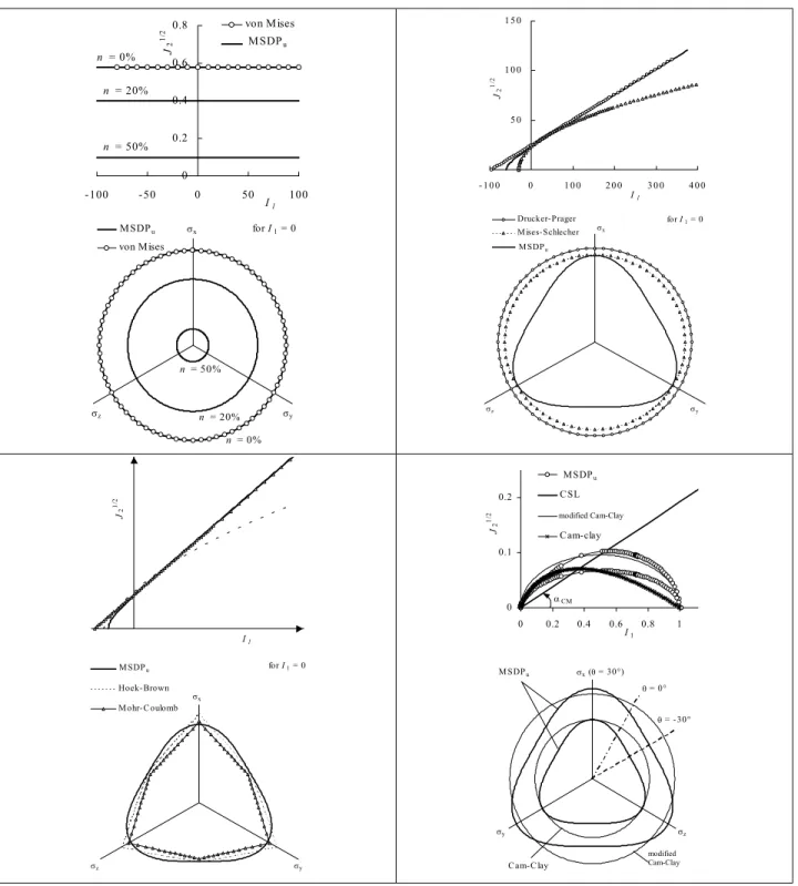
Figure 8. Graphical comparison between the MSDPu criterion and various existing criteria (shown for normalised parameters). 0 0.2 0.4 0.6 0.8 -100 -50 0 50 100 I1 J2 1/ 2 von Mises M SDPu n = 0% n = 20% n = 50% von Mises MSDPu σx for I1 = 0 σy σz n = 50% n = 20% n = 0% 0 5 0 1 0 0 1 5 0 - 1 0 0 0 1 0 0 2 0 0 3 0 0 4 0 0 I1 J2 1/ 2 Drucker-Prager M ises-Schlecher M SDPu for I1 = 0 σx σy σz I1 J 2 1/ 2 Hoek-Brown M ohr-C oulomb M SDPu for I1 = 0 σx σy σz 0 0.1 0.2 0 0.2 0.4 0.6 0.8 1 I1 J2 1/ 2 C SL C am-clay modifié C am-clay αCM MSDPu modified Cam-Clay C am-C lay modifié M SDPu C am-C lay σx (θ = 30°) θ = -30° θ = 0° σy σz modified Cam-Clay

0 4 8 12 -10 -5 0 5 10 15 20 25 I1 J 2 1/ 2

DiM aggio et Sandler

MSDPuMSDPu

DiMaggio and Sandler

MS DPu Cap σx (θ = 3 0°) θ = -30° θ = 0° σy σz DiM ag gio a nd S and ler 0 0.2 0.4 0.6 0.8 0 1 2 3 4 I1 J 2 1 /2 MSDPu Gurson (1 97 7) Tvergaard (1 98 1) Tvergaard et N eedleman 1984

Tvergaard and N eedlemeant

MSDPu Gurson σx (θ = 30°) θ = -30° θ = 0° σy _σz Tvergaard (1981) Tvergaard et N eedleman (1984)

Tvergaard and Needlem eant

0 0 .2 0 .4 0 .6 0 1 2 3 I1

J21 /2 Shima and Oyane 1976

MSDPu n = 0.2 n = 0.1 MS DPu Shima a nd O ya ne 19 7 6 σx (θ = 3 0°) θ = - 3 0° θ = 0° σy σz 0 20 40 60 -10 190 390 590 790 990 I1 J 2 1/ 2 MSDPu Lee and Oung 2000

n = 0.2

n = 0.1

MS DPu

Lee and Oung 200 0

σx (θ = 30 °)

θ = -30° θ = 0°

0 0.2 0.4 0.6 0 2 4 6 I1 J21 /2 MSDPu H ansen e t al. 1998

Sofronis and Mc Meeking (1992)

n = 0.2 n = 0.1 MSDPu Hansen et al. 1998 σx (θ = 30°) θ = - 30 ° θ = 0 ° σy σz Sofronis and McMeeking (1 99 2) 0 40 80 120 0 100 200 300 400 I1 J 2 1/ 2 Lade SM P M SD Pu σx σy σz 0 20 40 60 -100 100 300 500 700 I1 J 2 1/ 2 MSDPu Ehlers 1995 MSDPu Ehler (1995) σx (θ = 30°) θ = -30° θ = 0° σy σz 0 100 200 300 400 500 -100 100 300 500 700 900 I1 J2 1/ 2 Desai MSDPu Desai M SDPu σx (θ = 30°) θ = -30° θ = 0° σy σz

0 10 20 30 -20 0 20 40 60 80 I1 J2 1/ 2 M SD Pu O ttosen σx σy σz

4. APPLICATION OF THE MSDPu CRITERION

4.1 Identification of MSDPu parameters

Like other criteria, the MSDPu criterion contains parameters determined experimentally. A general approach for obtaining the optimised parameters is presented by Li et al. (2000). Li and Aubertin (2003) also discuss a method for defining the values of σun (eq.7) for σcn and σtn (used in parameters a1n and a2n).

As shown in Figure 9, the surface of the MSDPu criterion deviates from the surface defined for low porosity materials when I1 ≥ Icn. The surface closes at I1n where the deviator is nil. Parameter a3n is also utilised to define the surface as a function of porosity n when the material is under hydrostatic pressure (see Fig. 6f). For a given value of I1n (for porosity n), one can obtain a3n from equations (2) – (6), as follow:

(

)

(

)

2 c 1 2 2 1 1 2 1 2 3 2 n n n n n n n I I a I a I a − + − α = (11)

The value of parameter I1n may be obtained from test results under hydrostatic compression, or deduced from tests under conventional triaxial compression (CTC, θ = 30°) or reduced triaxial extension (RTE, θ = -30°), for I1 > Icn.

To define the relationship between porosity and the values of I1n and Icn, equation (7) may be used or alternative relationships can be proposed. For instance, in soil mechanics, a logarithmic relationship between the void ratio e and the effective stress is often applied (e.g., Roscoe and Burland 1968; Wood 1990). In rock mechanics, exponential laws and power functions are often used (e.g., Li and Aubertin 2003).

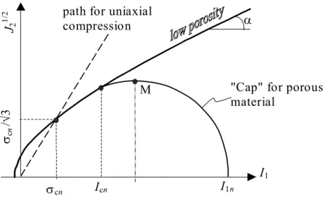
Figure 9. Schematical representation of the MSDPu criterion for dense and porous materials (with "Cap")

in CTC conditions (θ = 30°); the effect of porosity on the surface starts from Icn; the surface

closes on the I1 axis at I1n; the maximum value of J21/2 corresponds to point M. Other parameters

are also shown on the figure.

Icn I1n

I1

J2

1/

2

M "Cap" for porous material

α path for uniaxial

compression

σcn

σcn

/√

3

Physically, I1n and Icn tend towards infinity when porosity tends towards zero. This explains the absence of a Cap on the inelastic surface (in the I1-J21/2 plane) for materials with a very low porosity (such as hard rocks and certain types of concrete). When porosity n tends towards a critical value nC (<1), such as defined in equation (7), the material loses its uniaxial strength and I1n and Icn will then reach their minimum value.

Based on these considerations and analysis of available results, the authors have considered the following expressions for I1n:

              ₋ = sinh C 1 1 1 1 p ' n n n n I

I (newly proposed equation) (13)

where I'1n, q1 and p1 are material parameters.

Figure 10 shows the relationship between I1n and n for plaster under relatively high hydrostatic pressure. The three equations considered above are well correlated to the experimental results. Subsequently, in this report, equation (13) is retained because of its versatility and relative simplicity.

Figure 10. Variation of I1n with porosity of plaster; tests on cylindrical samples under hydrostatic

compression (ratio water/plaster = 70%) (data from Nguyen 1972); I '1n = 1052.9 MPa, nCc =

100%, x1 = 0.2847 and x2 = 14.225 with equation (7'); I '1n = 1604.5 MPa and q1 = 6.876 with

equation (12); I1n' = 50.6 MPa, nCc = 100%, and p1 = 0.898 with equation (13).

0 100 200 300 0.2 0.4 0.6 0.8 1 n I1n (M P a) données éq. (16) éq. (10) fonction exponentielle eq. (12) data eq. (7') eq. (13)

For Icn, it is postulated that the same functions may be employed. The relationship then becomes:               ₋ = 2 1 sinh C c c p ' n n n n I I (14) In equation (14) I '

cn and p2 are additional material properties. As there is little data available to experimentally define parameter Icn, it is postulated that parameters p1 and p2 take the same value (i.e. p1 = p2 = p). It is understood that the validity of this starting hypothesis must be confirmed by experimentation.

4.2 Graphical representation of experimental results

The following comparisons illustrate how the MSDPu criterion may be applied to describe the characteristic surfaces of materials with different porosity.

In the case of rocks and other brittle materials with very low porosity (n < 1 – 3%), the applicability of MSDPu has been well documented (Aubertin and Simon 1996, 1997, 1998; Aubertin et al. 1999, 2000). In this case the criterion can describe the condition of failure (see Fig. 11a) and the damage initiation threshold (onset of crack propagation, see Figs. 11b, 11c and 11d), without the closed portion on the positive I1 axis (i.e. Icn is very large).

Figures 17 to 20 show the use of MSDPu (with b = 0.75), for I1 > Icn, in the case of a rock (Fig. 17), plaster (Fig. 18), clay (Fig. 19), and residual soil (Fig. 20). In these cases, the surface closes on the I1 axis in compression.

Figures 21 through 23 show how the criterion may be used to describe the elastic limit and the failure condition for various materials, such as a porous rock (Fig. 21), an agglomerated residual soil (Fig. 22), and a paste cemented backfill (Fig. 23).

Finally, Figures 24 and 25 present the application of MSDPu to describe the strength of sand under different loading geometries.

These few illustrations demonstrate the ability of the MSDPu criterion to adequately describe the failure strength and the elastic limit of a wide variety of porous materials. Other examples of application have been presented by the authors in the publications cited above.

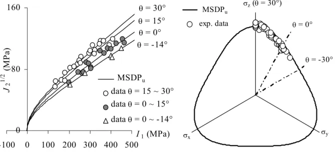
Figure 11a. MSDPu applied to the failure of sandstone, with σcn = 85 MPa, σtn = 2 MPa, φ ≈ 28°, b = 0.75,

Icn >>, v1 = 0 (data from Takahashi and Koide 1989).

0 80 160 -100 0 100 200 300 400 500 I1 (MPa) J2 1/ 2 (M P a) MSDP_u θ = 15° θ = 30° data θ = 0 ~ 15° data θ = 15 ~ 30° θ = 0° θ = -14° data θ = 0 ~ -14° exp. data θ = -30° θ = 0° σz (θ = 30°) σy σx MSDPu

Figure 11b. Application of the MSDPu criterion to describe the damage initiation threshold of a rock salt

submitted to CTC and RTE stress conditions (data from Thorel 1994); b = 0.75, φ = 0°,

σc = 15 MPa, σt = 1.5 MPa (after Aubertin and Simon 1997).

0 10 20 30 40 50 -50 0 50 100 150 200 250 I1 (MPa) J2 1/ 2 (M P a) data on a rocksalt CTC RTE MSDPu

Figure 11c. Application of the MSDPu criterion to describe the damage initiation threshold of a man-made

salt submitted to CTC stress conditions (data from Sgaoula 1997); b = 0.75, φ = 0°, σc = 37 MPa,

σt = 3 MPa. 0 10 20 30 40 50 -20 0 20 40 60 80 100 120 140 I1 (MPa) J2 1/ 2 (M P a)

data on man-made rocksalt

Figure 11d. Application of the MSDPu criterion to describe the damage initiation threshold of Lac du Bonnet grey granite submitted to CTC stress conditions (data from Lau and Gorski 1991); b = 0.75,

φ = 47°, σc = 70 MPa, σt = 3 MPa (after Aubertin and Simon 1997).

0 20 40 60 80 100 120 -20 30 80 130 180 230 I1 (MPa) J2 1/ 2 (M P a)

Lac du Bonnet grey granite

MSDPu

Figure 12. MSDPu and the failure strength (CTC) of crushed Westerly granite (data from Zoback and

Byerlee 1976) with b = 0.75, φ = 33.8°, σcn = 3.1 MPa, σtn = 0 MPa.

0 100 200 300 400 0 400 800 1200 I1 (MPa) J2 1/ 2 (M P a)

data on crushed W esterly granite

Figure 13. Description of the failure strength (CTC) of powdered aluminum with the MSDPu criterion (data

from Cristescu et al. 1996): a) aluminum A10 with φ = 35.5°, σcn = 27.4 kPa, σtn = 0 kPa; b)

aluminum A16-SG, with φ = 30°, σcn = 50 kPa, σtn = 0 kPa.

a) 0 200 400 600 800 1000 0 1000 2000 3000 I1 (kPa) J2 1/ 2 (k P a)

data on dense A10 alumina MSDPu aluminum A10 b) 0 300 600 900 0 1000 2000 3000 I1 (kPa) J2 1/ 2 (k P a)

data on dense A16-SG alumina

MSDPu

aluminum A16-SG

Figure 14. Failure strength of stiff Todi clay (CTC) and the MSDPu criterion (data from Rampello 1991): a)

for samples allowed to swell with φ = 51.5°, σcn = 0.093 MPa, σtn = 0 MPa; b) for undisturbed

samples with φ = 61.2°, σcn = 0.54 MPa, σtn = 0.037 MPa.

a) 0.4 0.8 1.2 J2 1/ 2 (M P a) b) 0.2 0.4 0.6 0.8 J2 1/ 2 (M P a)

Figure 15. Failure strength (CTC) of Ottawa sand and the MSDPu criterion (data from Wan and Guo 2001);

b = 0.75, φ = 26.6° (estimated), σcn = 1.9 MPa (estimated), σtn = 0 MPa, a3n = 0.0482 (estimated),

and Icn = 1156.6 MPa (estimated).

0 200 400 600 0 1000 2000 3000 4000 I1 (MPa) J2 1/ 2 (M P a)

data on O ttawa sand

MSDPu

Ottawa sand

Figure 16. Failure strength (CTC) of Sacramento River sand and the MSDPu criterion (data from Wan and

Guo 1998): a) for dense samples with φ = 35.8°, σcn = 196.67 kPa, σtn = 0 kPa, Icn > 12000 kPa; b)

for looser samples with φ = 29.1°, σcn = 43.67 kPa, σtn = 0 kPa.

a) 0 700 1400 2100 2800 3500 0 4000 8000 12000 I1 (kPa) J2 1/ 2 (k P a) data on dense

Sacramento River sand.

MSDPu dense sand 0 700 1400 2100 2800 0 4000 8000 12000 I1 (kPa) J2 1/ 2 (k P a)

loose Sacramento River sand

MSDPu b)

Figure 17a. Failure strength (CTC) of Indiana limestone and the MSDPu criterion (data from Schwartz 1964)

with φ = 35° (estimated), σcn = 38 MPa (measured), σtn = 3 MPa (estimated), a3n = 0.105

(estimated), and Icn = 40 MPa (estimated).

0 20 40 60 -10 190 390 590 I1 (MPa) J2 1/ 2 (M P a) Indiana limestone MSDPu

Figure 17b. Failure strength (CTC) of Weald shale and the MSDPu criterion (data from Madsen et al. 1989);

φ = 38° (estimated), σcn = 5 MPa (estimated), σtn = 0.1 MPa (estimated), a3n = 0.21 (estimated),

and Icn = 45 MPa (estimated).

0 5 10 15 20 25 J2 1/ 2 (M P a) Weald shale MSDPu

Figure 17c. Failure strength of normally consolidated (at 10 MPa) Trenton limestone and the MSDPu

criterion (data from Nguyen 1972); φ = 33° (estimated), σcn = 10 MPa (estimated), σtn = 0.5 MPa

(estimated), a3n = 0.134 (estimated), and Icn = 18 MPa (estimated).

0 5 10 15 -10 10 30 50 70 90 110 I1 (MPa) J2 1/ 2 (M P a) Trenton O rdovician limestone MSDPu

Figure 17d. Failure strength (CTC) of chalk and the MSDPu criterion (data from Elliott and Brown 1985);

φ = 28° (estimated), σcn = 8 MPa (estimated), σtn = 0.1 MPa (estimated), a3n = 0.125 (estimated),

and Icn = 11 MPa (estimated).

0 5 10 -5 15 35 55 I1 (MPa) J2 1/ 2 (M P a) chalk MSDPu

Figure 17e. Failure strength (in CTC) of limestone and the MSDPu criterion (data from Cheatham 1967); Icn =

0 MPa, σcn = 20 MPa, σtn = 0.5 MPa, φ = 28°, a3n = 0.102 for preconsolidated (at 34.5 MPa)

limestone; Icn = 0 MPa, σcn = 12 MPa, σtn = 0.5 MPa, φ = 28°, a3n = 0.09 for intact

(unconsolidated) limestone. 0 5 10 15 20 -10 20 50 80 110 I₁ (MPa) J2 1/ 2 (M P a) intact pré-consolidé à 35 MPa MSDP_u données (unconsolidated) preconsolidated at 35 MPa data

Figure 18. Failure strength (in CTC) of plaster samples (water/plaster = 50%) and the MSDPu criterion (data

from Nguyen 1972); description of intact plaster (n = 44.3%) with φ = 30° (estimated),

σcn = 13.6 MPa (measured), σtn = 2.6 MPa (measured), I1n = 79.6 MPa (measured) and Icn = 8

MPa (estimated); for preconsolidated plaster at 51.7 MPa (n = 32.25%) with φ = 30° (estimated),

σcn = 13.3 MPa (measured), σtn = 2 MPa (estimated), I1n = 154.9 MPa (measured) and Icn = 15

MPa (calculated). 10 15 20 J2 1/ 2 (M P a) n = 44.3% n = 32.25% MSDPu data

Figure 19a. Failure strength (in CTC) of Matagami clay and the MSDPu criterion (data from Nguyen 1972);

φ = 30° (estimated), σcn = 48 kPa (measured), σtn = 1 kPa (estimated), a3n = 0.9 (estimated) and

Icn = 180 kPa (estimated). 0 40 80 -10 90 190 290 I1 (kPa) J2 1/ 2 (k P a) Matagami clay MSDPu

Figure 19b. Failure strength (in CTC) of Leda clay and the MSDPu criterion (data from Nguyen 1972);

φ = 10° (estimated), σcn = 107.8 kPa (measured), σtn = 15 kPa (estimated), a3n = 0.9 (estimated)

and Icn = 530 kPa (estimated).

0 50 100 150 -10 190 390 590 790 I1 (kPa) J2 1/ 2 (k P a) Leda clay MSDPu

Figure 20a. Failure strength (in CTC) of basalt residual soil and the MSDPu criterion (data from Maccarini

1987); φ = 22.7°, σcn = 914.1 kPa, σtn = 127.4 kPa, a3n = 0.10 and Icn = 13.6 kPa.

0 200 400 600 -500 500 1500 2500 3500 I1 (kPa) J2 1/ 2 (k P a)

data on basalt residual soil.

MSDPu

Figure 20b. Failure strength (in CTC) of a gneiss residual soil and the MSDPu criterion (data from Sandroni

1981); φ = 24.5°, σcn = 119.9 kPa, σtn = 0.9 kPa, a3n = 0.09 and Icn = 45.4 kPa.

0 40 80 120 J2 1/ 2 (k P a) data on gneiss residual soil MSDPu

Figure 21a. Failure strength and elastic limit of Kayenta sandstone (in CTC) and the MSDPu criterion (data

from Wong et al. 1992); for failure: φ = 30° (estimated), σcn = 30 MPa (measured), σtn = 2 MPa

(estimated), a3n = 0 (or Icn >> ); for yield: φ = 30° (estimated), σcn = 30 MPa (measured),

σtn = 2 MPa (estimated), a3n = 0.115 (estimated) and Icn = 250 MPa (estimated).

0 200 400 600 -20 580 1180 1780 2380 I1 (MPa) J2 1/ 2 (M P a) yield failure yield failure exp. data MSDPu

Figure 21b. Failure strength and elastic limit of Bath stone samples (in CTC) and the MSDPu criterion (data

from Elliott and Brown 1985); for failure: φ = 30° (estimated), σcn = 15 MPa (measured),

σtn = 1 MPa (estimated), a3n = 0 (or Icn >> ); for yield: φ = 30° (estimated), σcn = 15 MPa

(measured), σtn = 1 MPa (estimated), a3n = 0.095 (estimated) and Icn = 0 MPa (estimated).

0 10 20 30 -5 15 35 55 75 95 I1 (MPa) J2 1/ 2 (M P a) yield failure yield failure exp. data MSDPu

Figure 21c. Failure strength and elastic limit of a tuff (in CTC) with the MSDPu criterion (data from

Pellegrino 1970); for failure: φ = 20° (estimated), σcn = 3.8 MPa (measured), σtn = 0.5 MPa

(estimated), a3n = 0 (or Icn >> ); for yield φ = 20° (estimated), σcn = 3.8 MPa (measured),

σtn = 0.5 MPa (estimated), a3n = 0.115 (estimated) and Icn = 6.5 MPa (estimated).

0 2 4 6 -2 3 8 13 18 23 I1 (MPa) J2 1/ 2 (M P a) failure yield failure yield exp. data MSDPu

Figure 21d. Failure strength and elastic limit of Epernay chalk in CTC with the MSDPu criterion (data from

Nguyen 1972); for failure: φ = 30° (estimated), σcn = 8 MPa (measured), σtn = 0.1 MPa

(estimated), a3n = 0 (or Icn >> ); for yield: φ = 30° (estimated), σcn = 8 MPa (measured),

σtn = 0.1 MPa (estimated), a3n = 0.55 (estimated) and Icn = 30 MPa (estimated).

15 20 25 1/ 2 (M P a) yield failure yield failure exp. data MSDPu

Figure 22. Failure strength and elastic limit of a residual (volanic conglomerate) soil (in CTC) and the

MSDPu criterion (data from Uriel and Serrano 1973); for failure: φ = 25° (estimated),

σcn = 300 kPa (measured), σtn = 5 kPa (estimated), a3n = 0 (or Icn >> ); for yield: φ = 25°

(estimated), σcn = 300 kPa (measured), σtn = 5 kPa (estimated), a3n = 0.063 (estimated) and

Icn = 100 kPa (estimated). 0 400 800 1200 -10 1990 3990 I₁ (kPa) J2 1/ 2 (k P a) failure yield failure yield exp. data MSDPu

Figure 23. Failure strength and elastic limit of paste fills (in CTC) and the MSDPu criterion (data from

Ouellet and Servant 2000); 6.5% cement tested at 28 days with φ = 23°, σcn = 580 kPa,

σtn = 50 kPa (for failure with a3n = 0 or Icn >> ; for yield with a3n = 0.14, and Icn = 100 kPa); 6.5%

cement at 3 days with φ = 32°, σcn = 200 kPa, σtn = 0.5 kPa (for failure with a3n = 0 or Icn >> ; for

yield with a3n = 0.14, and Icn = 100 kPa); 3% cement at 15 days with φ = 37°, σcn = 10 kPa,

σtn = 0 kPa (for failure with a3n = 0 or Icn >> ; for yield with a3n = 0.14, and Icn = 150 kPa).

0 200 400 600 800 -100 400 900 1400 1900 I1 (kPa) J2 1/ 2 (k P a) 28 days, 6.5% cement 3 days, 6.5% cement 15 days, 3% cement 28 days, 6.5% cement 3 days, 6.5% cement 15 days, 3% cement yielding failure data on yielding MSDPu data on failure

Figure 24. Failure strength of loose Monterey sand and the MSDPu criterion (n = 43.8%); σcn = 3 kPa, σtn =

0, φ ≈ 38°, b = 0.75, Icn >> (or a3n = 0), v1 = 0 (data from Lade and Duncan 1973).

0 100 200 300 400 500 0 500 1000 1500 I1 (MPa) J2 1/ 2 (M P a) MSDP_u θ = 30° θ = 0° θ = 0 ~ -30° θ = 0 ~ 30° θ = -30° data a) exp. data θ = -30° θ = 0° σz (θ = 30°) σx σy MSDP_u b)

Figure 25. Failure strength of dense Monterey sand and the MSDPu criterion (n = 36.3%); σcn = 160 kPa, σtn

= 0, φ ≈ 38°, b = 0.75, Icn >> (or a3n = 0), v1 = 0 (data from Lade and Duncan 1973).

0 200 400 600 800 0 500 1000 1500 I1 (MPa) J2 1/ 2 (M P a) MSDPu θ = 30° θ = -30° θ = 0 ~ 30° θ = 0 ~ -30° θ = 0° data a) exp. data θ = -30° θ = 0° σz (θ = 30°) σx σy MSDPu b)

4.3 Description and prediction with the MSDPu criterion

In the preceding sections, the MSDPu criterion was used to describe yielding or failure conditions of various materials. Such application typically consists in identifying the material parameters while minimising errors between the available experimental data and the calculated results (Li et al. 2000). Such a descriptive approach is relatively straightforward and easy to use when the functions are adequately formulated; it simply becomes a regression problem. This is the case with MSDPu, in which each parameter has a clear physical meaning.

In certain cases, it may be useful to predict an estimated strength value as a function of the influence parameters. For instance, when the basic parameters necessary for a descriptive application have been obtained, some of these parameters can be used to predict the material response under different loading conditions (e.g., from CTC to RTE) or at a different porosity. In the case of MSDPu, there is an explicit dependency of parameters a1n, a2n, a3n and Icn (or I1n) with respect to porosity n (see eqs.7, 7', 12 and 13).

It may be useful to illustrate, with a few examples, the method to obtain the necessary parameters to describe (and sometimes predict) the behaviour of materials with variable porosity using MSDPu. Figure 26a shows a description of uniaxial compressive strength variation for plaster as a function of porosity. The parameters obtained by regression from equation (7) are: x1 = 1.334, x2 = 16.013, σc0 = 27.35 MPa, n = 100%. The uniaxial tensile strength, σ = -6.3 MPa, is also estimated by

To evaluate the parameters for Icn as a function of porosity n, tests conducted at a given porosity (i.e. n = 44%) are used (with eq. 13);I1 44% = 82.4 MPa is then obtained. Parameters σc44% (= 16 MPa) and σt44% (= 2.7 MPa) can be calculated using equation (7), as shown in Figure 26. A regression on the series of data (at n = 44%) gives Ic 44% = 45 MPa, a3 44% = 0.480 (based on eq. 11) and φ = 30°. Using equation (14), one can also determine that I'cn = 27.64 MPa. All of the parameters required to predict the strength of this material at different porosity are now available. In Figure 26b, it is shown how the MSDPu criterion predicts the strength for the plaster at different n values. The correspondence between the predicted and measured strength is not perfect, but the procedure provides preliminary values that can be quite useful.

The same procedure has been used to describe (and predict) the behaviour of a sandstone. Figure 27a presents a description of the uniaxial compressive strength (eq. 7), with x1 = 1.21, x2 = 25.39, σc0 = 193.04 MPa, and nCc = 52%. The parameters have been obtained from data provided by Farquhar et al. (1993, 1994). Regression on data for Berea sandstone at n =10.5% in CTC gives σt10.5% = 3.8 MPa (the compressive values of x1 and nC obtained for σcn are also used for σtn), φ = 32°, Ic10.5% = 380 MPa. Equation (13) and the two measured parameters, I1 11% = 1619.6 MPa and I1 13% = 1299.3 MPa, are then used to obtain p1 = 0.4365 and I'1n = 538.6 MPa. Parameter I'cn may be deduced from equation (14) with Ic10.5% = 380 MPa (see Fig. 27b); I'cn = 126.4 MPa is then obtained. With these parameters, the MSDPu criterion may be used to predict other experimental results (see Fig. 27b). These predictions are fairly good, given the significant dispersion of the experimental data.

When Icn is very large or when the range of mean stress is too small (I1 < Icn), the closed portion of the failure or yield surface is not apparent in the I1-J21/2 plane. In this case, the number of parameters used to describe the behaviour of the material using MSDPu is reduced. For example, Figure 28 (a