HAL Id: hal-00914335
https://hal.inria.fr/hal-00914335v2
Submitted on 20 Jan 2014
HAL is a multi-disciplinary open access
archive for the deposit and dissemination of
sci-entific research documents, whether they are
pub-lished or not. The documents may come from
L’archive ouverte pluridisciplinaire HAL, est
destinée au dépôt et à la diffusion de documents
scientifiques de niveau recherche, publiés ou non,
émanant des établissements d’enseignement et de
the many-core era
Surya Narayanan Natarajan, Bharath Swamy, André Seznec
To cite this version:
Surya Narayanan Natarajan, Bharath Swamy, André Seznec. Modeling multi-threaded programs
exe-cution time in the many-core era. [Research Report] RR-8453, INRIA. 2013, pp.23. �hal-00914335v2�
0249-6399 ISRN INRIA/RR--8453--FR+ENG
RESEARCH
REPORT
N° 8453
December 2013programs execution time
in the many-core era
RESEARCH CENTRE
RENNES – BRETAGNE ATLANTIQUE
Surya Natarajan, Bharath Swamy, André Seznec
Project-Teams ALF
Research Report n° 8453 — December 2013 — 24 pages
Abstract: Multi-core have become ubiquitous and industry is already moving towards the many-core era. Many open-ended questions remain unanswered for the upcoming many-core era. From the software perspective, it is unclear which applications will benefit from many cores. From the hardware perspective, the tradeoff between implementing many simple cores, fewer medium aggressive cores or even only a moderate number of aggressive cores is still to debate.
Estimating the potential performance of future parallel applications on the yet-to-be-designed future many cores is very speculative. The simple models proposed by Amdahl’s law or Gustafson’s law are not sufficient and may lead to overly optimistic conclusions. In this paper, we propose a more refined but still tractable execution time model for parallel applications, the SNAS model. As previous models, the SNAS model evaluates the execution time of both the serial part and the parallel part of the application, but takes into account the scaling of both these execution times with the input problem size and the number of processors. For a given application, a few parameters are collected on the effective execution of the application with a few threads and small input sets. SNAS allows to extrapolate the behavior of a future application exhibiting similar scaling characteristics on a manycore and/or a large input set.
Our study shows that the execution time of the serial part of many parallel applications tends to increase along with the problem size, and in some cases with the number of processors. It also shows that the efficiency of the execution of the parallel part decreases dramatically with the number of processors for some applications.
Our model also indicates that since several different application scaling trends will be encountered, heterogeneous architectures featuring a few aggressive cores and many simple cores should be privileged.
Résumé : Comme les précédents modéles , le modéle SNAS évalue le temps déxécution de la partie á la fois en série et en paralléle de la partie de l’application , mais tient compte de la mise á l’échelle á la fois de ces temps d’exécution avec la taille du probléme d’entrée et le nombre de processeurs. Pour une application donnée , quelques paramétres sont recueillies sur la réalisation effective de l’application avec quelques fils et petits ensembles d’entrée . SNAS permet d’extrapoler le comportement d’une application future présentant des caractéristiques de mise á l’échelle sur une manycore similaires et / ou un grand ensemble d’entrée.
Notre étude montre que le temps d’exécution de la partie de série de nombreuses applications paralléles tend á augmenter avec la taille du probléme , et dans certains cas avec le nombre de processeurs . Il montre également que l’efficacité de l’exécution de la partie parallèle diminue considérablement avec le nombre de processeurs pour certaines applications.
Notre modéle indique également que depuis plusieurs tendances différentes applications d’échelle seront rencontrées , les architectures hétérogénes comportant quelques noyaux agressifs et des processeurs simples devraient être privilégiés.
1
Introduction
Design focus in the processor industry has shifted from single core to multi-core [15].Initially, multi-core processors were used only for high performance computation, but today they have become omnipresent in every computing device. Following this trend, the industry and academia has already started focusing on the so called many-core processors.
“Many-core” or “Kilo-core” has been a buzzword for a few years. Single silicon die featuring 100’s of cores can be on-the-shelf in a very few years. While 4 or 8-cores are essentially used for running multiple process workloads, many cores featuring 100’s of cores will necessitate parallel applications to deliver their best performance. Many-cores will be used either to reduce the execution time of a given application on a fixed working set (i.e to enable shorter response time) or to enlarge the problem size treated in a fixed response time (i.e., to provide better service). In order to extrapolate the performance of current or future parallel applications on future many cores, simple models like Amdahl’s law [1] or Gustafson’s law [6] are often invoked; Amdahl’s law:- if one wants to achieve better response; Gustafson’s law:- if one wants to provide better service. Both these models are rules of thumb. They have the merit to be very simple and provide a rough idea of the possible performance. But they are very optimistic models.
Therefore, there is a need for a slightly more complex model that still remains tractable through simple equations, but better reflects the effective behavior of applications. In this paper, we propose such a simple execution time model for parallel applications on many cores, the SNAS model. As previous models, the SNAS model relies on the simplistic assumption that the application can be split in two separate parts, the serial part and the parallel part. Unlike Amdahl’s law or Gustafson’s law, the SNAS model does not assume that the execution speed-up of a parallel application is linear. It also explicitly allows to model the fact that the execution time of the serial part of the application can depend on the problem size and also on the number of processors.
The SNAS model only uses six parameters to model the execution time of a given parallel application on a manycore for any problem size and any processor number, three parameters for characterizing the execution time of the serial part, three parameters for characterizing the parallel part. For a given application, these parameters can be collected through the execution of the application on a few threads and relatively small input sizes. The SNAS model allows to extrapolate the behavior of the same application or of a future application exhibiting similar scaling pattern running on 100’s or 1000’s of processors with very large problem size.
Our study on existing multithreaded parallel benchmarks also shows that there is a large variety of performance scaling for the parallel parts of the applications. Many applications cannot exhibit linear speed-up even for very large input size. We also show that there are applications for which the execution time of the serial part tends to increase along with the problem size and that sometimes the work in the serial section grows faster than the work in the parallel section. In a few cases, the execution time of the serial part slightly increases with the number of processors, further reducing the potential benefits of the parallel execution. Through applying the SNAS model to heterogeneous manycores, we also confirm that building many cores with many simple cores and few complex cores could be the most cost-effective tradeoff as argued by [8].
The remainder of the paper is organized as follows. Section 2 defines the serial and par-allel parts of a parpar-allel application. Section 3 presents the major user perspectives of parpar-allel application, fixed workload or scaled workload, and their respective translation in simple execu-tion time models, Amdahl’s law and Gustafson’s law. Secexecu-tion 4 reviews the other related work on multi-core performance modeling. In Section 5, we propose our SNAS model for execution time of parallel applications and our methodology to collect parameters from benchmarks. In
Section 6, we describe the case studies and different benchmark suites we studied. Section 7 reports the effective parameters that were collected on our set of benchmarks. We analyze the implication of these parameters on application potential scaling on a symmetric manycore. Then we illustrate the limitations and potential erroneous conclusions that could be drawn from both Amdahl’s and Gustafson’s laws. Section 8 illustrates the potential benefit that could be obtained on parallel applications from a heterogeneous architecture combining a few very complex cores with many simple cores. In Section 9, we describe the limitations of our SNAS model and a possible direction to improve it. Section 10 summarizes and concludes the paper.
2
What is sequential or serial part in a multi-threaded
pro-gram
Previously proposed execution time models as well as the SNAS model presented in this paper assume that the execution of an application can be arbitrarily split in a serial part and a parallel part. The serial part is constituted of the sections where only a thread is running. The parallel part consists of the sections where several threads can run concurrently.
In a multi-threaded program, three contributions to the sequential part can be discriminated at a very high granularity. First, the code executed by the main thread of the program before the threads are spawned and the final code executed after they are joined.
Second, after the parallel threads are spawned, the master or main thread may have execute some serial work to manage the worker thread pool or to execute some code after a global synchronization. This part of the application is often referred to as Region Of Interest.
Third, critical sections executed in a parallel section may involve serializations of the execu-tions for a few threads. However such critical secexecu-tions are unlikely to impose complete serializa-tion. Moreover such a serialization is unlikely to last very long.
To capture serial and parallel sections in the execution of a parallel application (Section 5.2), we use coarse grain monitoring of the threads and a heuristic to classify threads as active or inactive. Since critical section execution is generally quite short and/or concurrent with other active threads, the execution of critical sections will be generally classified in the parallel part of the application.
3
Fixed workload perspective versus Scaled workload
per-spective
Two simple models Amdahl’s law [1] and Gustafson’s law [6] are still widely used to extrapolate the theoretical performance of a parallel application on a large machine.
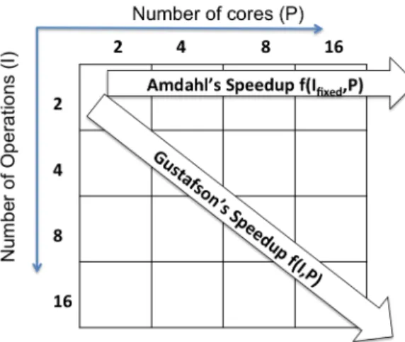
Amdahl’s law and Gustafson’s law are essentially two rules of thumb. They correspond to two very different views of the parallel execution of an application. We will refer to these two views as the fixed workload perspective and the scaled workload perspective respectively(illustrated in Fig. 1).
• Fixed workload perspective Amdahl’s law assumes that the input set size (workload) of an application remains constant for a particular execution. The objective of the user is to reduce the computation time through executing the program on a parallel hardware. This law corresponds to executing a fixed problem size as fast as possible.
• Scaled workload perspective Gustafson’s law assumes implicitly a very different scheme for parallel execution. The objective of the user is to resolve the largest as possible problem
in a constant time. In this perspective, it is assumed that the relative part of the parallel computations grows with the problem or input set size.
Both perspectives are valid but for different users. The whole spectrum of users requirements lies between users demanding ultimate fast answer for a given application workload and users demanding to resolve the largest possible problem in a given time frame.
Amdahl’s law was defined assuming the Amdahl’s perspective. The model determines the theoretical speedup of an application by considering a fixed amount of work done across varying number of cores, as shown in Fig. 1. The main observation from the model is that, speedup mainly depends on the size of the serial portion even if we assume infinite parallel computing resources, the execution time of a parallel application for a given problem size cannot be reduced below the execution time of the serial part of the program. Amdahl’s speedup is given by Eq. 1, where f stands for the fraction of parallel part in the program, and P is the number of cores of the machine on which the application is executed. In simple terms, for a given application, the maximum achievable speedup is determined by the fraction of serial part of the program. However, Amdahl’s law does not define what contributes to the serial part of the program.
speedup
Amdahl=
1
(1 − f ) +
Pf(1)
Through fixing the fraction of sequential code in an application, and considering that it cannot vary, Amdahl’s law seems to imply that there is no possibility to increase the performance of an application above a certain limit through parallelization. This is true under a fixed workload perspective.
On the other hand, Gustafson’s Law [6] presents a much more optimistic model which com-putes the speedup in terms of amount of work done.
Gustafson’s law assumes that the parallel part of the application increases linearly with the number of cores P as shown in Fig. 1 while the serial part remains constant. Gustafson’s speedup is given by Eq. 2, where, f is the fraction of time spent on executing the parallel part of the application on P processors and the rest 1 − f is spent on the serial part.
speedup
Gustaf son= (1 − f ) + f ∗ P
(2)
These two laws are used to provide contradictory arguments for focusing on designing more efficient cores (Amdahl’s law) or embedding more cores (Gustafson’s law).
However both Amdahl’s law and Gustafson’s law are based on very rough assumptions that do not correspond to the effective behavior of applications, and both are over-optimistic.
In particular, they assume that the execution time of sequential part of the application does not depend on the number of processors (Amdahl’s and Gustafson’s laws) and on the input problem size (Gustafson’s law). They also assume that the performance on the parallel part scales linearly when the number of processors grows (Amdahl’s and Gustafson’s laws).
These assumptions do not hold on real applications, even for limited thread numbers as we illustrate in Section 7. In Section 5, we present a more realistic model that includes serial scaling and parallel scaling.
4
Other Related Works
After the introduction of Amdahl’s and Gustafson’s laws, there was a debate on the validity of these laws [16], [18], [10]. [7] proposed memory bound speedup where the memory capacity is considered the dominant factor as they are also related to the problem size.
Figure 1: Amdahl’s law assumes a fixed workload while Gustafson’s law assumes scaled work-load.
Extending the Amdahl’s passive model, [8] propose a performance-area model called Amdahl’s law in the multicore era. This work mainly focuses on predicting the individual core size on the die which will yield maximum performance for the future applications on symmetric, asymmetric and dynamic multicore chips. The authors conclude that asymmetric or dynamic multicore chips are better tradeoffs than symmetric multicores.
[5] introduce a probabilistic model which shows that, even the Critical Section(CS) in the parallel part contributes to the serial section of the program. The study quantifies the serial part of the CS as the probability of a thread to enter a CS and the contention probability of other threads waiting to enter the same CS.
In [9], the authors provide a new direction to model program behavior. They extend Gustafson’s law to symmetric, asymmetric and dynamic multicores to predict multicore performance. They claim that neither the parallel fraction remains constant as assumed by the Amdahl’s law nor it grows linearly as assumed by Gustafson’s Law. Therefore, they propose the Generalized Scaled Speedup Equation (GSSE) as shown in Eq. 3. GSSE is s an intermediate model where the amount of work that can be parallelized is proportional to a scaling factor Scale(P)=√P. Their conclusion was that asymmetric and dynamic multicores can provide performance advantage over symmetric multicores. But again the impact of serial part is neglected in this model .
speedupGSSE=
(1 − f ) + (f ∗ Scale(P ))
(1 − f ) +(f ∗Scale(P ))P (3) [14] analyze the scalability of a set of data mining workloads that have negligible serial sections in the reduction phase of the program. It concludes that serial section in an application does not remain constant.
For our SNAS model, we build on the observation that not all applications are scaling the same way with the number of processors or the input set size problem. Therefore we try to characterize this scaling through a few parameters.
5
Performance Modeling of Parallel Application Execution
Time
As we move towards the many-core era, some analytical models are needed to estimate the poten-tial benefits of extending the applications and/or scaling the microarchitecture. The previously proposed models -Amdahl’s law, Gustafson’s law, Juurlink et al.’s GSSE- focus on the parallel part of the application and essentially neglect the possible variations of the execution time of the serial part in their performance models. They also assume linear speed-up on the parallel part.
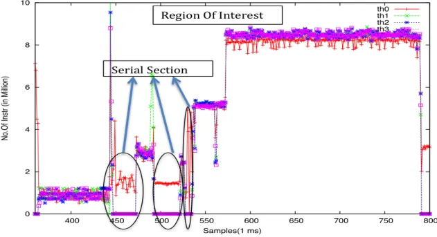
This simple modeling does not hold for many real- world applications. We analyzed the execution trace of available benchmark suites. On these traces, we noticed that for some appli-cations, the execution time of the serial section increases significantly with the input size, but also sometimes with the number of processors. As an example, Fig. 2 shows the execution trace of the Region Of Interest (ROI) in delaunay triangulation program of LONESTAR benchmark suite [11]. In this example, the program is executed with 4 threads each executing on a different core. It can be observed that sequential sections -as defined earlier in Section 2- are encountered within the ROI.
We also remarked that the efficiency of the parallel processors is not constant, but sometimes decreases dramatically with the number of processors. This leads us to propose a refined model of parallel application scaling, the SNAS model. The SNAS model is still simple assuming only one serial part and one uniform parallel part, but takes into account input set/problem size scaling and processor number scaling.
! 0 2 4 6 8 10 400 450 500 550 600 650 700 750 800
No.Of Instr (in Million)
Samples(1 ms) th0 th1 th2 th3 Region!Of!Interest! Serial!Section!
Figure 2: Delaunay Triangulation ROI showing the number of instructions executed by each thread and thread 0 executing serial part in between the parallel section
5.1
The SNAS Performance Model
Our model’s main objective is to extrapolate the multicore execution behavior of a parallel program to the future many-cores. To keep the model simple, we consider only input set size I and the number of processors/cores P . Therefore, SNAS just assumes a uniform parallel section and a uniform serial section, that is we model the total execution time as the sum of serial and parallel execution times as shown in Eq. 4.
t(I, P ) = tseq(I, P ) + tpar(I, P ) (4)
Both execution times tseq(I, P ) and tpar(I, P ) are complex functions. However, to keep it
simple, our model assumes that for both the execution times, the scaling with the input set size (I) and the scaling with the number of processors (P ) are independent. That is tseq and tpar
can be modeled as: tpar(I, P ) = Fpar(I) ∗ Gpar(P )and tseq(I, P ) = Fseq(I) ∗ Gseq(P ). Moreover,
our SNAS model assumes that F and G can be represented by a function of the form h(x) = xα.
Thus, the general form of execution time of the parallel execution is:
t(I, P ) = cseqIasPbs+ cparIapPbp (5)
The SNAS model only uses 6 parameters to represent the execution time of a parallel application, taking into account its input set and the number of processors. cseq, as and bs are used to model
the serial execution time and cpar, ap and bp are used to model the parallel execution time.
In the remainder of the paper, we will refer to respectively as and ap as the input serial scaling parameter, ISS and the input parallel scaling parameter, IPS. We will refer to respectively bs and bp as the processor serial scaling parameter PSS and the processor parallel scaling parameter PPS.
In particular, Amdahl’s law and Gustafson’s law can be viewed as two particular cases of the SNAS model.
A comparison with Amdahl’s Law Amdahl’s law assumes a constant input Ibase and an
execution time of the serial part independent from the processor number, i.e. bs = 0. It also assumes linear speedup with the number of processors on the parallel part, i.e bp = −1. In that context, f = cparIbaseap
cseqIbaseas +cparIbaseap .
A comparison with Gustafson’s Law Gustafson’s law assumes constant execution time cseq
for the serial part, i.e. independent of the working set (as = 0) and the number of processors (bs = 0). It assumes that the input is scaled such that 1) the parallel workload IGus executed
with P processors is equal to P times the “parallel" workload with one processor, i.e., Iap Gus= P.
2) speedup on the parallel part is linear, i.e. PPS bp = −1.
5.2
Extracting application parameters for the SNAS model
The SNAS model that we have defined above, should be used to extrapolate performance of (future) parallel applications on large many cores. However, one needs to use realistic parameters. Hence, we have performed such an evaluation on a set of parallel benchmarks.
The general methodology we use is as follows. We consider a parallel application and we execute it on a parallel execution platform. We execute it with various small number of threads and various small input sizes. The execution of the parallel and serial sections are monitored, i.e. tseq(I, P )and tpar(I, P )are measured for a range of different input sizes and different number
of threads. Then we use regression analysis with the least-square method to determine the best suitable parameters from the available experimental data.
Monitoring methodology Experiments are run with 2, 4, 8 and 16 threads and for 4 different input set sizes. All our reported experiments are performed on Intel(R) Xeon(R) CPU E5645 which has 2 sockets of 6 cores with 2 way SMT i.e up to 24 logical threads can run simultaneously. The operating system is Fedora Linux.
We use Tiptop [17] to obtain the run-time measurements from the Performance Monitoring Unit (PMU).
Tiptop [17] is a command-line tool for the Linux environment which is very similar to top shell command. Tiptop is built with the perf_event system library which is available in the Linux kernel. This system call lets Tiptop register new counters for processes running on the machine, and subsequently reads the value of the counters. Tiptop monitors all the necessary parameters of an attached process and periodically logs the values from the Performance Monitoring Unit which are then processed to get the desired metrics. Tiptop works on unmodified benchmarks from the outside and has only very marginal performance impact.Events can be counted per thread.We took samples every 1 ms to study the behavior of the benchmarks.
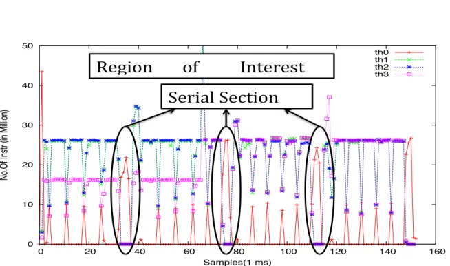
Determining whether the execution is serial or parallel is done empirically: on a given 1ms time slice, a thread is classified as active if it exceeds a minimum CPU utilization threshold (> 1%). For example, in Fig. 5, bodytrack benchmark is illustrated. th0 is the master thread and th1, th2, th3 are worker threads. We observe that in between the time samples 25-30, 60-65, 100-105 (approximately), the parallel threads are inactive and the master thread is active, thus contributing to the serial section.
In the next section, we present the benchmarks used in our experiments.
6
Parallel benchmarks
For this study, we focus on applications that will be executed on future manycores. Therefore we consider benchmarks which are parallelized with shared memory model using Pthreads library. We investigated two different categories of benchmark suites as our case study. They are 1. Regular parallel programs from the PARSEC benchmark suite and 2. Irregular parallel programs from the LONESTAR benchmark suite.
Multi-threaded programs have generally 3 major phases namely 1) the initialization phase where input data are read from input files or generated, data structures are then initialized, 2) the Region Of Interest (ROI) where the threads are created and main computation is executed and 3) the finalization phase where the threads are joined and further processing is run till the end of the program.
In all our analysis, we illustrate both the complete activity of the application and the activity restricted within the ROI, i.e. the activity of the program from the time the parallel threads are created until they are destroyed. The reported parameters for the ROI represent the portion of the code that was parallelized and is an optimistic evaluation of the potential speed-up, while the parameters reported for the complete application could be considered as a pessimistic evaluation since it includes artifacts such as benchmark packaging, input generation or read/write etc.
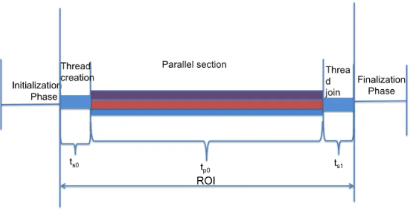
The behavior of the ROI depends on the parallelization technique used. On some applications, the data can be segmented and distributed to multiple threads running on multi-core after the initialization phase. In such applications, once the threads are spawned they work till the assigned job is complete without any intervention. As can be seen in Fig. 3, the serial part in the ROI is contributed only by thread creations and thread joins . Except for the initial data distribution, thread creation and thread join, most part of the work is executed in parallel. Therefore, here the contribution of serial section in the ROI is very small compared to the parallel section tp0.
Figure 3: The behavior of parallel applications without inner serial section
On the other hand, the applications that uses pipeline parallelism or a worker thread pool based implementation has a ROI which behaves like Fig. 4, where the master thread does some work to feed the worker threads. Here, the contribution of serial section in ROI can be very significant and is dependent on the amount of work the master thread. For example, the body-track program of PARSEC (Fig. 5) has serial intervention in the ROI. Again, our experimental measurements do not capture the serialization due to very fine grain synchronization.
Figure 4: Behavior of a parallel program using a worker thread pool
6.1
Regular Parallel programs
This class of applications operate on arrays and matrices where the data can be clearly partitioned and can be processed over multiple cores in parallel. We chose the PARSEC benchmark suite [3] for our study of regular programs. Most of the PARSEC benchmarks are data parallelized or pipeline data parallelized. Load balancing is managed statically. These benchmarks basically have an initialization phase consisting of reading data from file or generating data. Then the ROI begins in the parallel section.
We studied Bodytrack, Canneal, Fluidanimate, Raytrace, Streamcluster and Swaptions. The reason for the selection of these programs are further explained in Sec. 7. We noticed that Bodytrack was an exception among them. Bodytrack is a computer vision application which tracks the human movement by processing the input frame by frame. It implements a
worker-! 0 10 20 30 40 50 0 20 40 60 80 100 120 140 160
No.Of Instr (in Million)
Samples(1 ms) th0 th1 th2 th3
Serial!Section!
Region!!
of!! !
Interest!
Figure 5: Bodytrack showing the number of instructions executed by each thread and thread 0 executing serial part
thread pool where the main thread works like a master thread and the other threads are worker threads.
The run-time execution trace of Bodytrack is shown in Fig. 5. We can notice some serial sections where only the main thread is active. From our analysis, these sections are used to downscale the image before the output creation process. This serial section does scale with the input set size.
6.2
Irregular Parallel programs
Irregular programs operate over pointer-based data structures such as trees and graphs. The connectivity in the graph and tree makes the processing, memory access pattern data dependent and are unknown before the input graphs are known. Due to this reason, static compiler analysis fails to unveil total parallelism available in such applications. [13], [12] introduce the Galois run-time support system which can operate over the irregular programs to abstract the amorphous data parallelism by speculative or optimistic parallelization.
The LONESTAR [11] benchmark suite consists of irregular programs using the Galois run-time system to exploit the underlying parallelism. The operation of this run-run-time system is similar to the dynamic scheduling technique used on Out-of-Order processors. Galois run-time performs optimistic parallelization of programs containing Galois iterators. The run-time system builds the graph, schedules the nodes to be executed in different threads and speculatively executes the nodes in the graph. By speculatively executing code in parallel, the Galois approach can successfully parallelize programs exhibiting amorphous data-parallelism. However the cost of mis-speculation cannot be neglected in such systems. It becomes an extra scaling bottleneck for
the applications along with other issues like data locality and the synchronization of the data structure.
We studied 10 benchmarks in LONESTAR benchmark suite and noticed the serial scaling behavior in Delaunay Triangulation, Preflowpush, Independent set, Boruvka’s Algorithm, Max Cardinality Bipartite Matching and Survey propogation. On analyzing these benchmarks, we observed that the serial part of the program scales with the scaling of the input size in the ROI. In Delaunay Triangulation, serial part is mainly contributed by adding the points to the worklist and dividing the work. Periodically, the quad-tree needs to be updated with all the new points added to the mesh. The scalability is limited due the sequential generation of the quad tree. Preflowpush, Independent set, Boruvka’s Algorithm, Max Cardinality Bipartite Matching also had a bigger serial section. It can be attributed to the local graph computation which builds the customized graph for further parallelization. Time spent in the serial section depends on the input set scaling.
7
SNAS parameters for parallel benchmarks
We illustrate a subset of the PARSEC benchmarks and LONESTAR benchmarks. The two conditions that were necessary for our modeling are 1) Program should be able to run from 2 to 16 threads in individual cores, 2) input sets had to be generated with known scaling factors. This confines us with a choice of 6 PARSEC programs and 10 LONESTAR programs.
Several benchmarks from PARSEC and LONESTAR are not considered in our study. We use P for PARSEC and L for LONESTAR to distinguish the benchmark suite they belong. The reasons for not considering certain programs are as follows: Blackscholes (P), Discrete Event Simulation (L) has a constant small input set size that is too small to be measured, Facesim(P) has only one input set, Asynchronous Variational Integrators(L) has fixed input set which are not scalable, Dedup, X264 (P) had problems with number of spawned threads, Freqmine, Vips (P) were not buildable. Agglomerative Clustering, Delaunay Mesh Refinement (L) were producing erroneous results.
In the PARSEC benchmark suite, Bodytrack, Canneal, Fluidanimate, Raytrace, Streamclus-ter and Swaptions programs were satisfying our requirements. PARSEC benchmarks usually have 2 kinds of input set scaling 1) Complex component scaling 2) Linear component scaling.
Linear Component: It includes the part that has linear effect on the execution time of the program such as the number of iteration in the outer most loop of the workload. Complex component: It affects the execution time of the program i.e. it increases the work unit size and also the memory footprint.
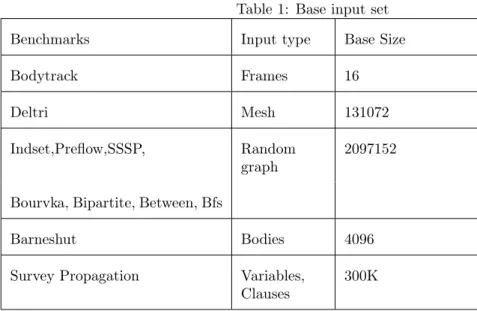
We used the linear component scaling in these applications, as they have a known scaling factor. Number of frames are varied linearly for bodytrack program of PARSEC benchmark suite as shown in Table. 1. Similarly, the respective linear components are scaled in Canneal, Fluidanimate, Raytrace, Streamcluster and Swaptions with reference to the information provided in Fidelity and Scaling of the PARSEC Benchmark Inputs[2].
For the LONESTAR programs, Table 1 shows the input set parameters utilized in the ex-periments along with their scaling factor. For example, Delaunay triangulation (deltri) program utilizes linearly varying mesh size. Independent set (indset) , preflowpush (preflow), Single-Source Shortest Path (sssp), Boruvka’s Algorithm (Bourvka), Max Cardinality Bipartite Matching (Bi-partite),betweeneness centrality (between)programs use randomly generated graph with linearly varying number of nodes. The number of bodies varies linearly in barneshut. Understanding the impact of this set of parameters on the execution time of each of the application is out of the scope of the paper; however the execution time measurements confirmed that for most
applica-Table 1: Base input set Benchmarks Input type Base Size Bodytrack Frames 16 Deltri Mesh 131072 Indset,Preflow,SSSP, Random
graph 2097152 Bourvka, Bipartite, Between, Bfs
Barneshut Bodies 4096 Survey Propagation Variables,
Clauses 300K
tions the parallel computation time (for a fixed number of threads) varies approximately linearly with the parameters that we varied. For barnes and between, the variation is quasi quadratic.
The number of cores are also varied from 2,4,8 and 16 to perform the experiments and to compute the SNAS model parameters.
Table. 2 reports the SNAS model parameters that were computed from our experiments on the 12 applications.
7.1
Analysis of specific cases
• 7 of the benchmarks do not exhibit any serial computation inside the region of interest: canneal, fluidanimate, raytrace, stream cluster, swaptions, sssp and bfs.
• The modeling of the measured execution times reported slight superlinear speedups for the parallel regions of Canneal, raytrace and swaptions, i.e bp > 1; we decided to treat this as measurement errors and report bp = 1.
• For some benchmarks (bodytrack,preflow,indset), the parameters reported considering the serial part of the complete application and the parameters reported for the ROI only serial part are very similar while they are significantly different for others. For these applications, the serial part before thread creation and after thread joining is quite dependent on the input set size.
• On fluidanimate, the execution time of the complete serial part depends on the number of processors.In that particular case, we verified in the source that some pre-treatment is dependent of the numbers of threads of the application: the initsim function computes partitioning based on the square root of number of threads.
• bodytrack has a very specific behavior: the serial section execution time decays with the number of processors. This is basically due to some overlapping between the serial section and the execution of the parallel section; the processor executing the serial section begins
Table 2: SNAS model parameters Complete application ROI
serial section Serial section Parallel section Bodytrack 103.29I0.9888P−0.2689 101.40I0.9956P−0.2714 608.405I0.9627P−0.6571 Canneal 5429.78I0.0018P0.0052 0 1499.28I0.9749P−1
Fluidanimate 26.4208I0.0960P0.1967 0 44.264I1.0353P−0.6536 Raytrace 5781.11I0.0244P0.0021 0 4857.32I0.9559P−1
Streamcluster 1.0441I1.4913P0.0565 0 2475.283I0.9427P−0.6839
Swaptions 3.2712I0.5696P0.0616 0 1453.06I0.9892P−1
Deltri 130.64I0.9048P0.0025 16.149I1.0630P0.1009 202.135I1.0544P−0.6963
Indset 20.41I1.1198P0.2463 18.553I1.0672P0.2646 355.7442I0.9844P−0.4931
Preflow 150.20I0.8568P0.1567 147.26I0.8366P0.1575 3399.71I0.9563P−0.6205
Barneshut 1.0877I1.3994P0.01324 2.253I0.3407P0.06184 520.012I1.9423P−0.7614
Sssp 39.6194I1.1023P0.0136 0 793.31I1.0118P−0.7633 Between 11.532I0.6161P0.0392 3.5275I0.8073P0.3234 549.42I2.3903P−0.4897
Bfs 55.403I1.0576P0.0129 0 602.84I1.0139P−0.6084 Boruvka 1045.25I0.9990P0.0098 0.5920I1.3287P0.0933 5382.49I1.0589P−0.7500
Bipartite 60.474I0.7443P0.0096 39.924I0.6416P0.2347 2457.33I0.7574P−0.7810 Survey 76.991I0.9027P0.0047 10.359I0.5917P0.2707 5375.37I0.6408P−0.5490
the down sampling of the image size for the output generation stage while some of the processors are still working on the parallel part.
7.2
Contrasting SNAS model with Amdahl’s and Gustafson’s laws
Tables 3 and 4 are illustrating the contrast between our SNAS model, Amdahl’s law and Gustafson’s law assuming 1,024 processors.
Table 3: Speedup in terms of Amdhal’s law, Gustafson’s law and SNAS model for n=1024, I=1 Complete application ROI
Benchmark f Amdhal’s Gustafson’s SNAS f Amdhal’s Gustafson’s SNAS body 0.855 6.85 875.52 31.76 0.85 6.95 877.84 32.49 Canneal 0.216 1.27 222.35 1.26 1.0 1024.0 1024.0 1024.0 Fluidanimate 0.626 2.67 641.68 0.68 1.0 1024.0 1024.0 92.81 Raytrace 0.457 1.83 468.08 1.81 1.0 1024.0 1024.0 1024.0 Streamcluster 1.0 715.4 1023.5 106.9 1.0 1024.0 1024.0 114.4 Swaptions 0.998 310.5 1021.70 8.51 1.0 1024.0 1024.0 1024.0 deltri 0.607 2.54 622.38 2.47 0.92 13.35 948.31 6.39 indset 0.946 18.11 968.4 3.02 0.95 19.80 973.29 2.92 preflow 0.958 23.12 980.7 7.22 0.95 23.55 981.52 7.31 barnes 0.997 225.3 1020.4 112.5 0.99 189.1 1019.5 85.43 SSSP 1.0 1024.0 1024.0 198.63 1.0 1024.0 1024.0 198.63 Between 0.979 46.47 1002.9 16.71 0.99 136.05 1017.4 10.70 Boruvka 0.837 6.11 857.6 5.59 1.0 920.43 1023.8 174.50 Bfs 0.916 11.77 938.03 9.48 1.0 1024.0 1024.0 67.86 Bipartite 0.976 40.04 999.4 33.29 0.98 59.00 1007.6 11.66 Survey 0.986 66.27 1009.5 27.37 0.998 344.9 1022.0 28.75
(except 1 and 10 for barneshut and between since their parallel execution scales quadratically with the input set). The fraction f of time spent on the parallel code used for Amdahl’s law and Gustafson’s law is also reported. f is computed by f = cparIbaseap
cseqIbaseas +cparIbaseap . We report the results
for the three models considering the ROI as well as for the complete application.
Directly applying Gustafson’s law or Amdhal’s law appears highly optimistic. In practice, assuming a linear speed-up on the parallel section is completely unrealistic: our measures show that many applications do not scale linearly even for 16 threads.
extrapo-Table 4: Speedup in terms of Amdhal’s law, Gustafson’s law and SNAS model for n=1024, I=100 Complete application ROI
Benchmark f Amdhal’s Gustafson’s SNAS f Amdhal’s Gustafson’s SNAS Body 0.839 6.19 859.5 29.64 0.838 6.125 857.8 29.81 Canneal 0.96 24.44 983.1 24.14 1.0 1024.0 1024.0 1024.0 Fluidanimate 0.992 112.4 1015.8 24.001 1.0 1024.0 1024.0 92.81 Raytrace 0.984 58.76 1007.5 57.92 1.0 1024.0 1024.0 1024.0 Streamcluster 0.995 160.8 1018.6 60.77 1.0 1024.0 1024.0 114.4 Swaptions 1.0 992.11 1023.9 383.6 1.0 1024.0 1024.0 1024.0 Deltri 0.755 4.07 773.4 3.915 0.923 12.88 945.5 6.18 Indset 0.903 10.24 925.0 1.776 0.929 13.91 951.42 2.107 Preflow 0.973 35.54 996.1 10.66 0.976 39.51 999.0 11.65 Barnes 0.999 507.7 1022.9 161.6 1.0 921.7 1023.8 189.7 SSSP 1.0 1024.0 1024.0 198.6 1.0 1024.0 1024.0 198.6 Between 1.0 752.3 1023.6 29.41 1.0 874.0 1023.8 28.47 Boruvka 0.872 7.733 892.5 7.024 1.0 736.8 1023.6 160.08 Bfs 0.899 9.829 920.8 8.093 1.0 1024.0 1024.0 67.86 Bipartite 0.977 42.37 1000.8 34.99 0.991 96.05 1014.3 19.06 Survey 0.954 21.45 977.2 14.61 0.998 398.31 1022.4 31.01
lates speed-ups higher than 773 on any of our benchmarks when considering the input set scaling by 100. Applying Amdahl’s law and contrasting tables 3 and 4 using different input set sizes would allow to get a slightly more realistic analysis. One can infer that some applications do not scale even if the input set size is increased: this corresponds to the applications for which the ISS and IPS parameters as and ap are equivalent e.g. deltri , preflow, boruvka .
In contrast, the SNAS model takes into account that the potential speed-up on the parallel section is sublinear i.e., that the PPS parameter bp > −1 for most of the benchmarks. Globally four different scaling behaviors are encountered on the benchmark set. They correspond to different PPS parameters bp (processor number parallel time parameters): bp1 for swaptions,
canneal and raytrace, bp34 for barneshut and sssp, boruvka and bipartite, bp23 for bodytrack, fluidanimate, streamcluster, deltri , preflow, and hfs, and bp12 for between, indset, survey. These four behaviors correspond respectively to maximum speed-ups for 1024 processors of respectively, 1024, 180, 100 and 32.
Due to the use of ISS and IPS parameters as and ap, the SNAS model also captures the correlation of both serial execution and parallel execution times with the input set size e.g. on deltri and preflow.
The SNAS model also takes into account the number of processors for executing the serial section. For instance, indset has a very low speedup due a non-negligible PSS parameter bs.
7.3
Fixed workload perspective
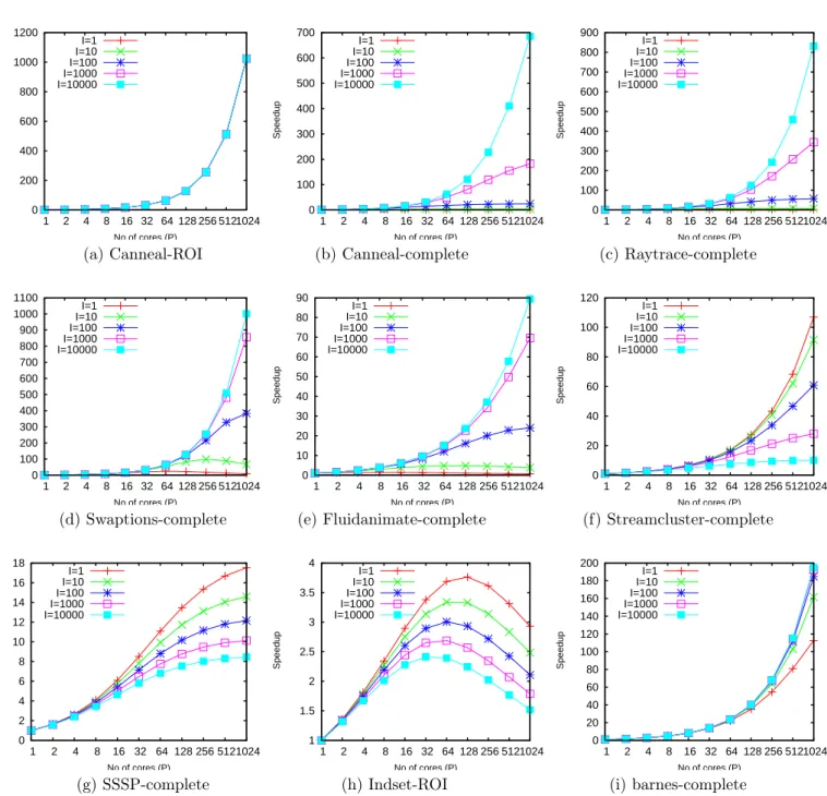
Figure 6 illustrates the potential speedups extrapolated for a few benchmarks varying the pro-cessor number from 1 to 1,024 and varying the problem size from 1 to 10,000. Some applications are illustrated considering only the ROI or the complete application. The illustrated examples are representative of the behaviors that are encountered.
For example, canneal encounters nearly perfect acceleration on the parallel part for every input set size, but large input set sizes are needed to amortize the initial and final phase. Similar behaviors are encountered for raytrace and to lesser extent for swaptions. This behavior may be deduced directly from the parameters of the applications. For canneal and raytrace, large cs
cp,
small ISS as and PSS bs - nearly independent of the serial section, ap close to 1 and bp close to -1, i.e., quasi linear scaling with input set size and the processor number. For swaptions, as is much smaller than ap while the initial cseq
cpar ratio is already small (short serial execution time
compared with parallel execution time on a single processor).
At a first glance, fluidanimate might be classified as encountering similar phenomenon (only the complete application is illustrated), needing a large input set to achieve a speed-up close to the one promised by its bp = −0.65 despite a serial section execution time increasing with the number of processors (bs = 0.2) but not with input set size.
It is often admitted that increasing the input set size of a parallel application translates into a higher speedup. This is not true. On many benchmarks, the work in the serial section grows at the same pace as the work in the parallel section e.g boruvka bfs (not illustrated).
Sometimes the work in the serial section even grows faster than the work in the parallel section. The poor scaling of streamcluster when considering the whole application with input set size can be explained by this phenomenon: as is around 1.5 while ap is only around 1. survey (not illustrated) and sssp suffer the same phenomenon. Some applications even multiply the difficulties for parallel execution scalability as Indset: the serial part grows faster than the parallel part when the input set increases (as > ap) and the serial part grows with the number of processors (bs = 0.26). On all these applications increasing the input set size decreases the speed-up that can be attained.
However when the execution time of the serial section is increasing with the input set, it does not always affect the scalability of the application. For instance, on barneshut, the execution of the serial section is also increasing with the input set size (as = 1.4 ) but at a much lower rate than the execution time of the parallel section (ap = 1.94).
7.4
Scaled workload perspective
Figure 7 illustrates the efficiency of a few benchmarks at constant execution time. That is, for a given number of processors, we first compute the maximum problem size that can be executed
0 200 400 600 800 1000 1200 1 2 4 8 16 32 64 128 256 512 1024 Speedup No of cores (P) I=1 I=10 I=100 I=1000 I=10000 0 100 200 300 400 500 600 700 1 2 4 8 16 32 64 128 256 512 1024 Speedup No of cores (P) I=1 I=10 I=100 I=1000 I=10000 0 100 200 300 400 500 600 700 800 900 1 2 4 8 16 32 64 128 256 512 1024 Speedup No of cores (P) I=1 I=10 I=100 I=1000 I=10000
(a) Canneal-ROI (b) Canneal-complete (c) Raytrace-complete
0 100 200 300 400 500 600 700 800 900 1000 1100 1 2 4 8 16 32 64 128 256 512 1024 Speedup No of cores (P) I=1 I=10 I=100 I=1000 I=10000 0 10 20 30 40 50 60 70 80 90 1 2 4 8 16 32 64 128 256 512 1024 Speedup No of cores (P) I=1 I=10 I=100 I=1000 I=10000 0 20 40 60 80 100 120 1 2 4 8 16 32 64 128 256 512 1024 Speedup No of cores (P) I=1 I=10 I=100 I=1000 I=10000
(d) Swaptions-complete (e) Fluidanimate-complete (f) Streamcluster-complete
0 2 4 6 8 10 12 14 16 18 1 2 4 8 16 32 64 128 256 512 1024 Speedup No of cores (P) I=1 I=10 I=100 I=1000 I=10000 1 1.5 2 2.5 3 3.5 4 1 2 4 8 16 32 64 128 256 512 1024 Speedup No of cores (P) I=1 I=10 I=100 I=1000 I=10000 0 20 40 60 80 100 120 140 160 180 200 1 2 4 8 16 32 64 128 256 512 1024 Speedup No of cores (P) I=1 I=10 I=100 I=1000 I=10000
(g) SSSP-complete (h) Indset-ROI (i) barnes-complete Figure 6: Fixed workload perspective for varying input set size from I = 1 to 10,000. Speed-up scale differs on the different graphes
in a constant time T from the SNAS model. Then we compute the speed-up on this workload over a sequential execution.
The execution times T considered varies from 1 to 10,000 seconds. We illustrate the same benchmarks as in Figure 6.
0 200 400 600 800 1000 1200 1 2 4 8 16 32 64 128 256 512 1024 Speedup No of cores (P) T=1s T=10s T=100s T=1000s T=10000s 0 200 400 600 800 1000 1200 1 2 4 8 16 32 64 128 256 512 1024 Speedup No of cores (P) T=1s T=10s T=100s T=1000s T=10000s 0 200 400 600 800 1000 1200 1 2 4 8 16 32 64 128 256 512 1024 Speedup No of cores (P) T=1s T=10s T=100s T=1000s T=10000s
(a) Canneal-ROI (b) Canneal-complete (c) Raytrace-complete
0 200 400 600 800 1000 1200 1 2 4 8 16 32 64 128 256 512 1024 Speedup No of cores (P) T=1s T=10s T=100s T=1000s T=10000s 0 10 20 30 40 50 60 70 80 90 100 1 2 4 8 16 32 64 128 256 512 1024 Speedup No of cores (P) T=1s T=10s T=100s T=1000s T=10000s 0 10 20 30 40 50 60 70 80 1 2 4 8 16 32 64 128 256 512 1024 Speedup No of cores (P) T=1s T=10s T=100s T=1000s T=10000s
(d) Swaptions-complete (e) Fluidanimate-complete (f) Streamcluster-complete
0 2 4 6 8 10 12 14 1 2 4 8 16 32 64 128 256 512 1024 Speedup No of cores (P) T=1s T=10s T=100s T=1000s T=10000s 1 1.5 2 2.5 3 3.5 1 2 4 8 16 32 64 128 256 512 1024 Speedup No of cores (P) T=1s T=10s T=100s T=1000s T=10000s 0 20 40 60 80 100 120 140 160 180 200 1 2 4 8 16 32 64 128 256 512 1024 Speedup No of cores (P) T=1s T=10s T=100s T=1000s T=10000s
(g) SSSP-complete (h) Indset-ROI (i) barnes-complete Figure 7: Scaled workload perspective for varying input set size from T = 1s to 10,000s
A clear observation can be drawn for the applications that exhibit benefits in terms of speedups from input set scaling: to achieve high efficiency for large number of processors (e.g. 90 % of the theoretical maximal Pbp speed-up), one will have to also increase the tolerated
re-sponse time of its application: curves T=1s and T=10s illustrate this phenomenon, for instance fluidanimate, canneal and raytrace.
7.5
Summary
We list here a small set of rules of thumb to analyze the expected scaling behavior of a parallel application from its SNAS model parameters:
• Maximum speed-up is limited by bp: bp close to -1 leads to potential linear speed-up, bp close to 0.5 limits the potential speed-up to the square root of the processor number. • The serial section work may scale with the input set size: if it scales with the same factor
as the parallel section (as ≈ ap), speed-up will not increase with the problem size. • The serial section can scale with the number of processors: if bs is non-negligible then it
will limit the effective speed-up.
8
SNAS model and Heterogeneous architectures
Mixing a few large complex and many simple cores has been proposed in the literature in order to speed-up the execution of serial sections in parallel applications [9].
[8] proposes an extension to Amdhal’s law for multi-core with an analytical model considering the area-performance relationship. They consider BCE, Base Core Equivalent, with a perfor-mance factor of 1. They assume that a core of r BCE will have a perforperfor-mance perf(r) with perf(r) = p(r), following Borkar’s rule of thumb [4].
The SNAS model can be used to evaluate the performance of such a hybrid multicore with a complex core executing the serial code. The execution time of an application on a processor with an area P BCE featuring one rs BCE core (executing the serial part and 1 thread of the parallel part) and rp-BCE cores (executing only threads of parallel part) will be modeled as:
thyb(I, rs, rp, P ) = cseqIas(1 +P −rsrp )bs √ rs + cparIap(1 +P −rsrp )bp √ rp (6)
Figure 8 illustrates the performance of a few benchmarks on several architectures featuring from 32 BCEs to 1024 BCEs areas. The illustrated architectures are Small-sym, a symmetric multicore built with small cores (1 BCE), med-sym, a symmetric multicore built with medium cores (4 BCEs), Small-hyb a hybrid multicore featuring small cores (1 BCE) and one complex cores (16 BCEs), Med-hyb a hybrid multicore featuring medium cores (4 BCE) and one complex core (16 BCEs). Input set size is chosen as 100.
As expected, applications that scales perfectly with the number of processors on the parallel section benefit from using small cores on the ROI (see canneal, swaptions and raytrace have very similar behaviors). However, once the complete serial part is taken into account, the performance on the serial section becomes a major consideration. When the number of core grows and the heterogeneous multicore gains momentum being able to achieve much higher performance than the symmetric architecture equivalent cores. On these applications, Small-hyb i.e simple 1-BCE cores associated with a complex 16-BCE core outperforms Med-hyb i.e. medium 4-BCE cores associated with a complex 16-BCE core.
On applications exhibiting lower scalability, our modelization confirms that an hybrid archi-tecture performs better than a symmetric archiarchi-tecture as soon as the area of the processor is large enough, large enough being 32 BCE or 64 BCE depending on the benchmarks. On the illustrated set of benchmarks, Small-hyb seems to outperform Med-hyb, except marginally for applications exhibiting very low potential speed-up parameter bp and suffering from a serial section partially scaling with the number of processors (indset, fluidanimate and preflow).
0 200 400 600 800 1000 1200 32 64 128 256 512 1024 Speedup BCE Small-Sym Med-Symm Small-Hyb Med-Hyb 0 200 400 600 800 1000 1200 32 64 128 256 512 1024 Speedup BCE Small-Sym Med-Symm Small-Hyb Med-Hyb 0 200 400 600 800 1000 1200 32 64 128 256 512 1024 Speedup BCE Small-Sym Med-Symm Small-Hyb Med-Hyb
(a) Canneal-ROI (b) Raytrace-ROI (c) Swaptions-ROI
0 10 20 30 40 50 60 70 80 90 100 32 64 128 256 512 1024 Speedup BCE Small-Sym Med-Symm Small-Hyb Med-Hyb 0 50 100 150 200 250 32 64 128 256 512 1024 Speedup BCE Small-Sym Med-Symm Small-Hyb Med-Hyb 0 100 200 300 400 500 600 700 800 900 1000 32 64 128 256 512 1024 Speedup BCE Small-Sym Med-Symm Small-Hyb Med-Hyb
(d) Canneal-complete (e) Raytrace-complete (f) Swaptions-complete
1 2 3 4 5 6 7 8 9 32 64 128 256 512 1024 Speedup BCE Small-Sym Med-Symm Small-Hyb Med-Hyb 0 10 20 30 40 50 60 32 64 128 256 512 1024 Speedup BCE Small-Sym Med-Symm Small-Hyb Med-Hyb 0 5 10 15 20 25 30 35 32 64 128 256 512 1024 Speedup BCE Small-Sym Med-Symm Small-Hyb Med-Hyb
(g) Indset-complete (h) Fluidanimate-complete (i) Preflow-complete Figure 8: Heterogeneous architecture potential, input set I=100
Therefore, applying the SNAS model on our application benchmarks confirms that an het-erogeneous architecture featuring a few complex cores and a large number of simple cores might be a good tradeoff for designing future large many-cores.
9
SNAS model limitations
We have developed the SNAS model in order to extrapolate the performance of future parallel applications on large scale many cores featuring 100’s or even 1000’s of cores. It is our belief that future applications will in some way exhibit scaling characteristics within the same spectrum as the benchmarks we studied in this paper.
However the SNAS model remains very rough and should be used very carefully when drawing definite conclusions on the scaling of a given application on a many core. Extrapolating the performance of a given application that was designed to run on a 10-20 core machine on such a large scale machine might be very risky, particularly when they are optimistic.
For example, the SNAS model is able to predict that if the PPS parameter bp is largely lower than 1 (e.g. bp = −0.5 ) or if the serial section is scaling with the input set and the processor number, then, the application is very unlikely to scale favorably with the number of processors and/or the input set. But, if the measured parallel scaling factor bp is close to -1 and the serial scaling is very limited then a sudden limitation can appear due to some unforeseen bottleneck such as memory bandwidth, locks contentions, cache contentions ..etc.
Moreover, the measured parameters are for a specific implementation of an architecture. Changing the balance in the architecture -e.g. cache per processor ratio, bandwidth per processor-can change the scaling parameters of the application. Application reengineering and algorithm modification will also change the scaling factors of an application.
Finally, the model could be refined for applications exhibiting several phases (including serial and parallel phases).
10
Conclusion
Multi-cores are everywhere and next generations of PCs and servers might feature tens or even hundreds of core. Parallelism is now the path for higher single application performance. How-ever, the traditional models for extrapolating parallel application performance on multiprocessor-Amdahl’s and Gustafson’s laws - are very rough and may be very misleading.
Not every application features a serial part that is independent of the input size and the number of processors. Additionally, performance on parallel part does not generally scale per-fectly linear with the number of processors. Our SNAS model allows to capture various scaling behaviors of applications depending on the input size I and number of cores P. We recall here this simple modelization:
t(I, P ) = cseqIasPbs+ cparIapPbp (7)
The SNAS model only uses 6 parameters to represent the execution time of a parallel application, taking into account its input set and the number of processors. cseq, asand bs are used to model
the serial execution time and cpar, apand bp are used to model the parallel execution time.
Through run-time monitoring, we have been able to empirically extract the parameters for parallel benchmark applications on a real system. Our model indicates that there exist some applications that will probably scale correctly on a 1000’s core processor (bp close to -1). But it also indicates that despite near optimal linear speed-up on the parallel part, global performance could be quite disappointing due to the scaling of the sequential part with the input set size ( significant ISS parameter as and even in the same range as the IPS parameter ap) and even with the number of processors (PPS parameter bs non null). It also shows that for other applications there is no hope for large performance increase with 1000 cores (e.g. bp in the -0.5 range).
On the architectural side, the SNAS model shows that symmetric many cores using very simple cores will only be able to achieve very high performance on a very specialized class of applications. For the spectrum of parameters that we encountered in our benchmark set, the SNAS model confirms that using an heterogeneous architecture featuring many simple cores and a few more complex cores could be the right tradeoff for future many cores as advocated in [8].
From the application side, we hope that the SNAS model will help application designers to understand how their application performance will scale with the number of cores and with the input set problem on future many-cores. Moreover a SNAS-like analysis of a complex multi-phase parallel application could help the application developer team to isolate the different potential bottlenecks for achieving high performance on a large manycore.
References
[1] Gene M. Amdahl. Validity of the single processor approach to achieving large scale comput-ing capabilities. In Proceedcomput-ings of the April 18-20, 1967, sprcomput-ing joint computer conference, AFIPS ’67 (Spring), pages 483–485, New York, NY, USA, 1967. ACM.
[2] C. Bienia and K. Li. Fidelity and scaling of the parsec benchmark inputs. In Workload Characterization (IISWC), 2010 IEEE International Symposium on, pages 1–10, 2010. [3] Christian Bienia, Sanjeev Kumar, Jaswinder Pal Singh, and Kai Li. The parsec benchmark
suite: Characterization and architectural implications. In Proceedings of the 17th interna-tional conference on Parallel architectures and compilation techniques, pages 72–81. ACM, 2008.
[4] Shekhar Borkar. Thousand core chips: a technology perspective. In Proceedings of the 44th annual Design Automation Conference, DAC ’07, pages 746–749, New York, NY, USA, 2007. ACM.
[5] Stijn Eyerman and Lieven Eeckhout. Modeling critical sections in amdahl’s law and its im-plications for multicore design. In Conference Proceedings Annual International Symposium on Computer Architecture, pages 362–370. Association for Computing Machinery (ACM), 2010.
[6] John L. Gustafson. Reevaluating amdahl’s law. Commun. ACM, 31(5):532–533, May 1988. [7] Xian he Sun and L.M. Ni. Another view on parallel speedup. In Supercomputing ’90.,
Proceedings of, pages 324–333, 1990.
[8] Mark D Hill and Michael R Marty. Amdahl’s law in the multicore era. Computer, 41(7):33– 38, 2008.
[9] B.H.H. Juurlink and C. H. Meenderinck. Amdahl’s law for predicting the future of multicores considered harmful. SIGARCH Comput. Archit. News, 40(2):1–9, May 2012.
[10] S. Krishnaprasad. Uses and abuses of amdahl’s law. J. Comput. Sci. Coll., 17(2):288–293, December 2001.
[11] Milind Kulkarni, Martin Burtscher, Calin Casçaval, and Keshav Pingali. Lonestar: A suite of parallel irregular programs. In Performance Analysis of Systems and Software, 2009. ISPASS 2009. IEEE International Symposium on, pages 65–76. IEEE, 2009.
[12] Milind Kulkarni, Martin Burtscher, Rajeshkar Inkulu, Keshav Pingali, and Calin Casçaval. How much parallelism is there in irregular applications? SIGPLAN Not., 44(4):3–14, Febru-ary 2009.
[13] Milind Kulkarni, Keshav Pingali, Bruce Walter, Ganesh Ramanarayanan, Kavita Bala, and L Paul Chew. Optimistic parallelism requires abstractions. In ACM SIGPLAN Notices, volume 42, pages 211–222. ACM, 2007.
[14] M. Manivannan, B. Juurlink, and P. Stenstrom. Implications of merging phases on scalability of multi-core architectures. In Parallel Processing (ICPP), 2011 International Conference on, pages 622–631, 2011.
[15] Jeff Parkhurst, John Darringer, and Bill Grundmann. From single core to multi-core: prepar-ing for a new exponential. In Proceedprepar-ings of the 2006 IEEE/ACM international conference on Computer-aided design, ICCAD ’06, pages 67–72, New York, NY, USA, 2006. ACM. [16] JoAnnM. Paul and BrettH. Meyer. AmdahlÕs law revisited for single chip systems.
Inter-national Journal of Parallel Programming, 35(2):101–123, 2007.
[17] Erven Rohou. Tiptop: Hardware Performance Counters for the Masses. Rapport de recherche RR-7789, INRIA, November 2011.
Campus universitaire de Beaulieu