Université de Montréal
Collaborative filtering techniques for drug discovery
par
7M/t(
3’/7
Durnitru Erhan
Département d’informaticiue et de recherche opérationnelle faculté des arts et des sciences
IViémoire présenté à la Faculté des études supérieures ell vue de l’obtention du grade de Maître ès sciences (M.$c.)
en informatique
Août, 2006
/1-(n
DUniversité
(111
de Montréal
Direction des bibliothèques
AVIS
L’auteur a autorisé l’Université de Montréal à reproduire et diffuser, en totalité ou en partie, pat quelque moyen que ce soit et sur quelque support que ce soit, et exclusivement à des fins non lucratives d’enseignement et de recherche, des copies de ce mémoire ou de cette thèse.
L’auteur et les coauteurs le cas échéant conservent la propriété du droit d’auteur et des droits moraux qui protègent ce document. Ni la thèse ou le mémoire, ni des extraits substantiels de ce document, ne doivent être imprimés ou autrement reproduits sans l’autorisation de l’auteur.
Afin de se conformer à la Loi canadienne sur la protection des renseignements personnels, quelques formulaires secondaires, coordonnées ou signatures intégrées au texte ont pu être enlevés de ce document. Bien que cela ait pu affecter la pagination, il n’y a aucun contenu manquant.
NOTICE
The author of this thesis or dissertation has granted a nonexclusive license allowing Université de Montréal to reproduce and publish the document, in
part or in whole, and in any format, solely for noncommercial educational and research purposes.
The author and co-authors if applicable retain copyright ownership and moral rights in this document. Neither the whole thesis or dissertation, nor substantial extracts from it, may be printed or otherwise reproduced without the author’s permission.
In comptiance with the Canadian Privacy Act some supporting forms, contact information or signatures may have been removed from the document. While this may affect the document page count, it does not represent any loss of content from the document.
Université de Montréal
FBculté des études supérieures
Ce mémoire intitulé:
Collaborative ifitering techniques for drug discovery
présenté par:
Dumitn Erhan
a été évalué par un juq composé des personnes suivantes:
Douglas Eck
président-rapporteur
Yoshua Bengio
directeur de recherche
Phifippe Langlais
membre du jury
RÉSUMÉ
Cette thèse examine le problème d’apprendre plusieurs tâches simultanément, afin de transférer les connaissances apprises à une nouvelle tâche. Si on suppose que les tâches partagent une représentation et qu’il est possible de découvrir cette représentation efficacement, cela peut nous servir à construire un meilleur modèle de la nouvelle tâche. Il existe plusieurs variantes de cette méthode: transfert induc tif, apprentissage multitâche, filtrage collaboratif, etc. Nous avons évalué plusieurs algorithmes d’apprentissage supervisé pour découvrir des représentations partagées parmi les tâches définies dans un problème de chimie computationelle. Nous avons formulé le problème dans un cadre d’apprentissage automatique, fait l’analogie avec les algorithmes staildards de filtrage collaboratif et construit les hypothèses générales qui devraient être testées pour valider l’utilisation des algorithmes mul titâche. Notis avons aussi évalué la performance des algorithmes d’apprentissage utilisés et démontrons qu’il est, en effet, possible de trouver une représentation partagée pour le problème considéré. Du point de vue théorique, notre apport est une modification d’un algorithme standard—les machines à vecteurs de support— qui produit des résultats comparables aux meilleurs algorithmes disponibles et qui utilise à fond les concepts de l’apprelltissage multitâche. Du point de vue pratique, notre apport est l’utilisation de notre algorithme par les compagnies pharmaceu tiques dans leur découverte de nouveaux médicaments.
Keywords: Apprentisage multitâche, Filtrage collaboratif, QSAR, Méthodes à noyaux, Réseaux de neurones
ABSTRACT
We investigate the problems of learning several tasks simultaneously in order to transfer the acquired knowledge to a new task. Assuming that the tasks share some representation that we can discover efficiently, such a scenario should lead to a better model of the new task, as compared to the model that is learned by oniy using the data for the new task. This technique has many names: inductive transfer, multi-task learning, learning to learn, collaborative filtering. Ail of these are varieties of the same idea that we try to exploit. We have evaluated several sllpervised learuing algorithms in order to discover shared representations among the tasks defined in a computational chemistry/drug discovery problem. We have cast the problem from a statistical learning point of view, traced analogies with standard collaborative filtering techniques, and set up the general hypotheses that have to be tested in order to validate the multi-task learning approach. We have then evaluated the performance of the learning algorithms and showed that it is iudeed possible to learn a shared representation of the tasks. from a theoretical point of view, our contribution also comprises a modification to the Support Vector Machine algorithm, which eau produce state-of-the-art resuits using multi-task learuing concepts at its core. from a practical point of view, our contribution is that this algorithm eau be readily used by pharmaceutical companies for virtual screening carnpaigns.
Keywords: Multi-task learning, Content-based filtering, QSAR, Ker nel Perceptroii, SVM, Neural Networks
CONTENTS RÉSUMÉ ABSTRACT CONTENTS LIST 0F TABLES.. LIST 0F FIGURES LIST 0F ABBREVIATIONS NOTATION DEDICATION ACKNOWLEDGEMENTS CHAPTER 1: INTRODUCTION 1.1 Machine Learning
1.2 Multi-Task learning and Collaborative 1.3 Drug Discovery
1.4 Multi-Target Virtual HTS 1.5 Contributions of the Thesis 1.6 Structure of the Thesis
CHAPTER 2: PREVIOUS WORK
2.1 Multi-task Learning
2.2 Collaborative and Content-Based Filtering 2.3 Virtual High-Throughput Screening/QSAR.
111 iv V viii ix xi xii xlii xiv 1 1 3 4568 Filtering 9 912 15
vi CHAPTER 3: PROPOSED ALGORITHMS
3.1 Formai Definition
Multi-Task Neural Network An inpiit-task simiiarity measure JRank
Multi-Task Support Vector Machines Partial Least Squares
CHAPTER 4: EXPERIMENTS 4.1 Experimentai Setup
4.1.1 Datasets and Descriptors 4.1.2 Task Selection
4.1.3 Undersampling Scheme 4.1.4 Hyper-Parameter Selection 4.1.5 Performance Measures 4.1.6 Target descriptors influence 4.2 Experimental Resuits
4.2.1 Task Selection
4.2.2 Multi-Task Neurai Network 4.2.3 JRank
Multi-Task Support Vector Machines Target Descriptors’ Influence
Zero-data experiments Comparison of ail algorithms
CHAPTER 5: DISCUSSION AND FUTURE 5.1 Discussion
5.2 Futllre Work
5.2.1 MT-SVM considerations 5.2.2 A neural network extension 5.2.3 Other avenues 18 181921242832 33 333335363738394141424346465153 WORK 3.2 3.3 3.4 3.5 3.6 4.2.4 4.2.5 4.2.6 4.2.7 57 57 58 59 60 60
vii
CHAPTER 6: CONCLUSION 62
LIST 0F TABLES
4.1 Comparillg MT-NNet’s performance with and without target de
scriptors 43
4.2 Lifts obtailled by testing on a completely new target with no trainillg
data 53
4.3 Comparison of ail multi-target methods with $T-$VM and PLS.
Lifts computed at tfractionrrO.9 56
4.4 Comparison of ail multi-target methods with ST-SVM and PL$.
LIST 0F FIGURES
2.1 Simple multi-task learning neural net 10
3.1 Multi-task Neural Network architectures 19
3.2 Intuition behind the update mie of JRank 27
3.3 Intuition behind the Multi-task Support Vector Machine approach 29 4.1 Number of compounds available for each target 34
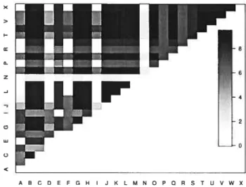
4.2 Number of compounds shared by each pair 41
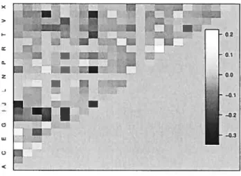
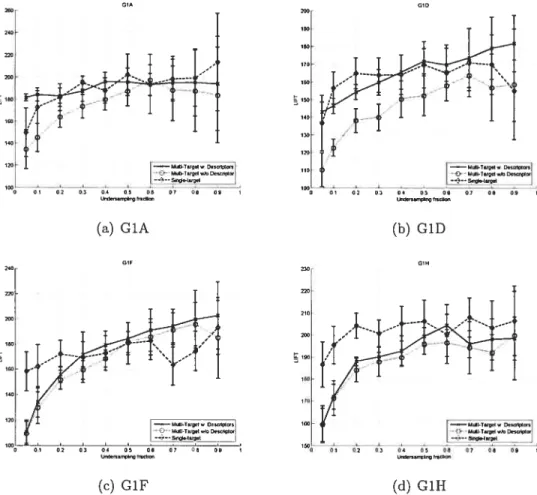
4.3 Pairwise Correlation of Biological Activity 42 4.4 Neural Net undersampling on G1A, GÏD, G1F, G1R 44
4.5 Neural Net undersampling on GlI, GiS, GlU 45
4.6 JRallk undersampling on GÏA, GÏD, Gif, G1H 47
4.7 JRank undersampling on Gil, GiS, GlU 48
4.8 SVM undersampling on G1A, G1D, Gif, G1H 49
4.9 SVM undersampling on G1I, GiS, Glu 50
4.10 Target descriptors influence for G1A, G1D, Gif, G1H with MT-SVM 51 4.11 Target descriptors influence for GlI, G1S, GlU with MT-SVM 52 4.12 Comparison of algorithms, G1A, G1D, G1F, G1H 54
4.13 Comparison of algorithms, GlI, GiS, GlU 55
LIST 0F ALGORITHMS
1 JRank 26
LIST 0F ABBREVIATIONS
CF Collaborative Filtering HTS High-Throughput Screening MTL Multi-Task Learning
MT-NNet Multi-Task Neural Network
MT-SVM Multi-Task Support Vector Machine MT-JRallk Multi-Task JRank
NNet Neural Network
QSAR Quantitative Structure-Activity Relationships ST-SVM Single-Task Support Vector Machille
$T-NNet Single-Task Neural Network $T-JRank $ingle-Task JRank
NOTATION
General:
R The set of real numb ers
X E R’ A d-dimensiona1 vector iII R, which contains input features
t E RDt A dt-dimensional vector in R, which contains task features
y A real number that is the the olltpnt corresponding to some pair (x,t)
Transpose of a vector/matrix
K(x, y) A kernel function evaluated for vectors x and y
‘I’(x, t) Map of a pair of vectors (x,t) to a (high-dimensional) feature vector
F(x,t;w) A linear transformation of I’(x, t), using w
f(x, t;w,
)
A decision function for (x,t)ACKNOWLEDGEMENTS
This thesis would have not been possible withollt the continiing support and guidance of my supervisor, Yosliua Bengio. My collaboration with Pierre-Jean L’Heureux was especially fruitful and enjoyable. Olivier Delalleau lias been the person without whom many of the experiments described in this thesis would not have been possible. The time spent in the USA and GAMME labs and the dis cussions with the guys auJ girls from there have certainly made the life more interesting throughout the whole master’s program. Many thanks to ail of you.
I woild also like to thank Dr. Christopher Walpole and other AstraZeneca R&D Montreal staff for offering me the opportunity to work on this very interesting dataset. This work was sllpported financially in part by Vatorisatiori Recherche
Québec auJ the National Science and Engineering Research Council of Canada. Last, but not least, I am very grateful to my parents and my girl-friend, who were of great help and provided lots of moral support during the last years!
CHAPTER 1
INTRODUCTION
The idea of learning more than one thing at a time is certainly not new. It is very likely that our brain does this constantly. We wanted to explore this idea in a more mathematical setting and apply our findings to a novel and very practical problem. This chapter introduces the reader to the general problem of learning and presents the setting and the motivation for onr work on Mnlti-Task Learning or Collaborative Filtering for drug discovery. We describe the main contributions of this thesis and we gnide the reader throngh the rest of the chapters.
1.1 Machine Learning
IVlachine Learning is the art of crafting techniques that allow compnters to “learn”. Cenerally speaking, it is a field of Artificial Intelligence that is closely re lated to the field of Statistics. IViachine Learning (ML) is typically concerned with bnilding algorithms for analyzing, deducing or inferring from data. Thns, Machine Learning research encompasses a broad spectrum of problems, such as the theoret ical fonndations of inference from data, the practical indnstrial considerations of learning algorithms, such as redncing their complexity, the analysis of the capacity of an algorithm to “learn” and to “generalize”, the definitions of “learning” and
“generalization”, etc.
A most general and, at the same time, precise definition of “learning” is not in the scope of this thesis. However, it is intuitively clear that we can daim that, for instance, a decision-making algorithm is “learning” if the decisions of this algorithm, based on the data from which it has “learned” something, are at least better than randomness and at best as good as (or better than!) the ones made by a human that has access to the same data as the algorithm. In the long rnn, a “learning algorithm” shonld produce decisions that are better and better over
2 time, as more and more data is used for building these decisions.
An example of such a decision-making algorithm is one that distinguishes apples from oranges. A human that has seen neither would probably be able to distinguish these fruits after seeing one or at most a few examples of each. It seems that our brain is able to learn these kinds of things very quickly—perhaps by comparing and contrasting the different properties of these fruits. Properties such as the generai shape (spherical or not), size, color, etc. could be used for constrllcting a “learning algorithm” that could use them in such a way so as to be able to ctassify a new example: either as an apple or as an orange. Presurnably, the algorithm would combine the properties iII a way that would reveal the connectioll between these
properties and whether the given fruit is an apple or an orange. This algorithm would also presumably become better and better at classifying fruits as it will have more data to fine-tune the parameters that uncover the relationship between their properties and their identity.
This simple exampie introduces many of the concepts alld problems that are fre quently encountered in Machine Leariling. The decision-making process of deciding which fruit is which is generally called classification. The phase of the algorithm that adjusts the parameters is called training. Choosillg a set or a function of the parameters that performs best is vatidation. The process of verifying how weii an algorithm works with a chosen set of parameters on new cases is cailed testing. The
generatization performance of an algorithm given a set of parameters and data for training and validatioll can then be estimated during testing.
There are many aspects of Machine Learning that have been overlooked when describing this example; we have not touched on what and how many properties of objects should we consider, whether we can performe classification without knowing the labels (the ideiltities) of the objects to be classified (by, for instance, clustering
them), whether the number of such labels can be greater than one (muÏti-cÏass
classification) or even infinite (regression), whether learning is ail about decision making or not, etc. We need not consider these things for now—the big picture is that, more often than not, it is desirable to buiid algorithms that have a good
3
generalization performance.
Given such an algorithm, it would be interesting to kllow the answer to the followillg questiolls: is it possible to “re-use” the “knowledge”, which one acquired by building this modet of the data, for learning a new task? The human brain seems to do it on a regular basis and this is a plausible explanation for our ability to classify apples and oranges from very few training examples. Natllrally, we would like a leariling algorithm to do the same. It turns out that there exist methods for learning more than mie task at a time and for transferring the acqiired “knowledge” between the tasks that are learned. We discuss this in more detail in the next section.
1.2 Multi-Task learriing and Collaborative Filtering
Multi-Task learning is known iinder a variety of names: learning to learn, in ductive transfer, bias learning, collaborative filtering, etc. Each of these notions are small variations of the same idea—that one can construct learning techniques that can exploit acquired “knowledge” in order to bias the learning of a new task and improve the generalization performance. A more detailed treatment of the pre vious work in the field of Multi-Task Learning is presented in Chapter 2; for 110W,
it suffices to say that the fteld was popularized in the 1990s by extending [15, 16] standard Neural Networks for learning multiple tasks at the same time.
$uch work lias shown theoretically and practically [8, 32] that taking into ac count multiple related tasks can be greatly beneficial to generalization, if the tasks are sufficiently related’. If the added tasks are unrelated, the generalization power could decrease, because spurious relations are learned, but there are cases when even unrelated tasks might be helpful [16].
One popular application of MTL are Collaborative Filtering [34, 60] systems.
‘A necessary and sufficient condition for task relatedness is roughly the following: there exists a simpler—perhaps in the Kolmogorov complexity [49] sense—model that describes the joint distribution of inputs, outputs, and tasks, than the separate models of inputs and outputs that one would obtain for each task.
4 $uch systems produce recommendations that are based on similarities between the preferences of different users of the system. Collaborative Filtering applications are usually online bookstores, movie rentais web-sites, onhine music shops, etc. where users of the system rate the products and where the system lias to infer the ratings that a user would give to the items he/she lias not rated yet. It is quite easy to draw the parallel between CF and MTL—predicting the preferences of one user is a single learning task, whereas modeling jointly the preferences of ail tlie users of the system could be considered multi-task learning. As we will see later on, this observation enabled us to extend a collaborative filtering algorithm that we then applied to solving a particular multi-task learning problem that lias very littie in common with user preferences; in what follows, we present the practical motivation for our work.
1.3 Drug Discovery
The pharmaceutical industry is a multi-billion industry that relies heavily on new computer technology both in the process of drug development and in the process of finding drugs for new or establislied diseases. The drug discovery process cari extend for several years and cari cost short of a billion dollars for a single drug. It is thus quite desirable for a pharmaceutical company to apply metliods for reducing tlie time and money spent on developing a new drug. Machine Learning techniques tliat help in building statistical models for evaluating potential drugs’ likelihood of success is one of the computational approaclies used in tlie industry.
Que of the first stages of drug discovery is called High-Throughput Screen ing (HT$), during which a library of usually tens of thousands of compounds is tested against tlie target protein—whici represents the “disease” that one tries to find a drug for—so that one cari see how much the componnds influence this tar get. Based on these results, one will try to develop a better compound by finding quantitative structure-activity relationships (Q$AR), i.e. correlations between the biological activity and the structure of the chemical compounds tlirough statistical
5 means. These correlations enable the drug discoverer to model the link between the structure and the activity and find compounds whose structures correspond to a more desirable level of activity.
Even given the recent advances in robotics, the process of physically testing each compound is time-consuming and expensive. Combinatorial chemistry2 tech niques allow us to produce (virtually) millions of compounds. Statistically reliable and computationally feasihie methods for performing “virtual screens” of these compounds are increasingly used in the pharmaceutical industry [13j. Virtual High-Throughput Screening is the process of building a model that “connects” the moledular features or structures (perhaps even the geometrical structures) of the compounds to their activity in the presence of a certain target.
Virtual HTS is in itself not an easy task, even if it usually does not involve a lot of laboratory work. This is because a reliable set of already tested compounds (the “training set”) has to be present, the molecular features of these compounds have to be representative, and the statistical model has to be able to link these features to the activity in the presence of a certain target such that it can generalize well to previously unseen compounds. There has been a lot of work and sticcess in applying Machine Learning methods to Virtual HTS problems. A round-up of these methods is presented in Section 2.3; for now, it suffices to say that the developments of the pharmaceutical research in this field follow very closely the developments in the Machine Learning community. This shows quite clearly that the pharmaceutical
industry is always in need for new technologies that would enable cornpa.nies to perform Virtual HTS campaigns more efficiently.
1.4 Multi-Target Virtual HTS
One interesting way of performing Virtual HTS more efficiently lies in exploit ing the data from previous HT$ campaigns. If these campaigns were performed on a set of related targets (we define such relatedness in Section 2.3) then it should be
6 possible to transfer—in an inductive way, as described in Section 1.2—the knowl edge acquired from the experiments to the virtual tests that are to be done on a new target (that is also related in some way to the targets for which we have experimental resuits). Such an algorithm could be put to good use by the pharma ceutical companies and in Section 2.3 we describe several scenarios in which such inductive transfer could help.
The parallel between collaborative filtering or multi-task learning and QSAR
/
Virtual HT$ eau be made almost immediately: the tasks (or the “users”) are the biological targets, the inputs (or the “items”) are the molecular compounds and the labels/outputs (or the “ratings”) are the levels of activity of the given compound for a given target. The descriptors or the features of the targets and of the compounds could be anything that might help us in uncovering relationships both between the targets and the compounds.1.5 Contributions of the Thesis
This work builds up on our article [27] and two poster presentations [26,48] on the same topic and which cover the first parts of the thesis.
In this thesis, we investigate several questions related to the process of multi task learning. First and foremost, we were interested in developing practical meth ods for measuring the degree to which we eau profit from learning multiple tasks at the same time. Therefore, it is very interesting for us to sec the evolution of the generalization of a multi-task learning algorithm when trained with only a small sample of data from a given task, as a function of the size of this sample. We are also interested in how it is possible to “transfer” the “knowledge” acquired by learning several tasks to a compÏetety new task. Finally, we wanted to explore theoretical and practical ways of eneoding the similarity or the relatedness of tasks and exploiting this for improving the multi-task learning algorithms that we used. We have demonstrated that “pure” inductive transfer is possible in the context of a particular application, and that it eau be quite helpful. We have defined a
7 clear way of testing, for a particular dataset, the degree to which multi-task learning helps, when compared to standard single-task learning. Ail the algorithms that we used have built-in ways of computing a similarity measure between tasks; one of these algorithms, the Multi-Ta.sk Support Vector Machine that uses a Collaborative Filtering-inspired kernel matches the state-of-the-art performance and is a clear candidate for inclusion into the industrial process of drug discovery.
from the point of view of the drug discovery process, our objective and contribu tion was to compare and evaluate methods to take advantage of the commonalities between the different targets within a target class. In addition, we deveioped a soiution that allows us to estimate QSAR models for so-calied “orphan targets” that have not yet been tested, or for which there are very httle available data. The goal of our approach was not to create the best global predictive model for a collec tion of accurately known targets. We assumed that we do not know the structure of the targets, because we want to generalize to a new unknown target. We have thus developed a practical approach where very little prior knowledge of the target is needed; we were less interested in building the best model for a single target than building a modei for which we lack sufficient data. Finaiiy, to the best of our knowledge, such a (muiti-target) dataset has neyer been discussed before in the computationai chemistry literature. This thesis (along with the afore-mentioned journal paper and presentations) is therefore the first to offer insights into this kind of dataset and ways to soive probiems defined by it.
To summarize: from the theoreticai point of view, our contribution is the anal ysis of Multi-Task Learning when one of the tasks is either compietely unknown to the learning aigorithm or for which we have only a smaH training set. Practically speaking, we tested a well-known Muiti-Task learning algorithm (MT-NNet) and modified a published algorithm (MT-JRank) to produce the Multi-Task Support Vector Machines which achieves state-of-the-art results for a novel drug discovery probiem. This aigorithm is aiso enabling us to conciude that, for the given drug discovery dataset, “pure inductive transfer” is possible, which is a very promising result.
$ 1.6 Structure of the Thesis
This thesis starts with an overview of the work donc iii the field of Multi-Task
Learning/Collaborative Filtering. Sections 2.1 and 2.2 discuss the developments in this field, from the flrst Neural Network-based models to the more modem kernel based approaches, and contain an overview of the theoretical irisights behind Multi Task Learning. Section 2.3 contains a short listing of the methods that have been used for solving the Virtual HTS problem. Finally, Section 2.4 draws the parallels between the research pmesented in the previous sections and this thesis.
We then proceed to formally describe the problem to be solved in Section 3.1. Sections 3.2, 3.4, 3.5 present the techniques that we used: a Multi-Task Neu rai Network, a kemnel perceptron-based Collabomative Filtering algorithm called JRank, and a Multi-Task Support Vector Machine. In Section 4.1 we discuss the experimental setup that is common to ail the algorithms, whereas in Section 4.2
we present the experimentai results obtained with each of the techniques.
Chapter 5 is a disdllssion of the resuits. We anaiyze possible extensions of our techniques and future directions of work in Section 5.2 and we conclude the thesis with Chapter 6, which summarizes the work clone and the resuits obtained.
CHAPTER 2
PREVIOUS WORK
In this chapter, we will go through the main developmellts of multi-task learn ing and collaborative ifitering, analyze the main ways that Machine Learning tech niques are used in the computational chemistry/drug discomulvery community, suggest ways of applying multi-task learning/collaborative ifitering techniques to solving the drug discovery problem using multiple related biological targets auJ trace parallels from our approaches to the previous work clone in the fteld.
2.1 Multi-task Learning
Que of the first attempts at constructing an efficient procedure for learning more than one task at a time was by extending standard multi-layer neural net works [62]. Neural networks provided an ideal testbed for implementing multi-task intuitions: there existed an efficient algorithm for training them, the translation of intuitions into concrete models was relatively easy and the multi-task models were computationally not much more expensive than simple, single-task learning models.
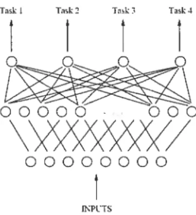
The simplest of such extensions was to create a shared hidden layer that is trained in parallel for ah the learnillg tasks. Figure 2.1 (taken from [16]) presents such an extension. In this case, the training procedure would be clone on all the tasks in parallel and because the structure of the network includes a shared layer (weight matrix), it is possible for so-called “shared internal representations” to develop alld to be learned. There are other architectures possible, but most, if not all of them are varieties of the same idea: that the tasks share some connections in the neural network. Caruana [16] provides a host of examples of such networks, and convincing results that show that such networks can mdcccl learn several tasks at the same time, better than equivalent single-task learning networks.
10
Taskl Iask2 Task3 Iask1
t
t
t
t
00000 000
00000000
INPUTS
Figure 2.1: A simple extension to the standard single-layer ileural network architec ture, which allows for multiple tasks to be learned at the same time, thus creating a so-called “shared internai representation”
A parallel development [7] (but in a Bayesian framework) introduced the notioll
of an objective TWT distribution, from which a learner samples the related tasks
that are to be learned. This enviroument that contains the sampled tasks provides
the multiple datasets that correspond to these tasks. Given this learner and a way to sample from such an environment, the learner can then search for the hypothesis that best explains the tasks. The same paper gave bounds on the information needed to iearn a task, when it is learned concurrently with other tasks. Baxter [9] then expanded on that and gave bounds on the number of tasks that are sufficient in order to learu a novel task. These resuits lay the theoreticai foundations for multi task learning and generalized the insights gained from extellded neural networks to handie multiple tasks.
Bakker [2] lias expanded on the intuitions behind the mlllti-task neural networks and behind the theoretical resuits of Baxter and lias introduced a hierarchical Bayes model that can also perform clustering of tasks. This is done by setting the prior over the shared parameters in a multi-task neural network as a mixture of Gaussians. The model can also account for more fine-grained relationships between tasks. This is obtained by introducing task-specific features and setting the first
11 moments of the priors a.s a function of these features.
Ben-David and $chuller [10] demonstrated a set of simple transformations that defined task retatedness. Their approach is based on comparing the distributions that generate the data for the tasks and using the similarity between these dis tributions to present bounds on how much a learning algorithm ca profit from performillg multi-task learning. Their approach is interesting as it provides a way of quantifying (albeit by a very simple measure) the relatedness of tasks.
The task relatedness idea can be viewed from a slightly different angle in the context of kernel machines [70]. Evgeniou, Micchelli, and Pontil [28,29] generalized the popular Support Vector iViachine algorithm [65] to use similarity measures and objective functions that take into account multiple tasks. They achieve this by using a regularized functional that couples the tasks and provides for a very explicit way of specifying the type of relatedness between tasks. Their approach can also accommodate for non-linear kernels. Their approach is also one of quite a general way of explicitly stating the relationships between tasks.
Multitask learning has been also been applied in a variety of settings. Predicting pneumonia mortality is a popular example [19], but fields as varied as sensor fusion for robotics [21], stock selection [33] and lifelong learning [67] have also profited from the algorithms developed in this field.
Most of the techniques that we just described attempt to use multi-task learning in order to improve the generalization performance of a task that encompasses them ail (muiti-task learning is viewed as learning a “common goal”, in a sense). As laid out in the introduction, our goal is to find a way to transfer the knowledge acquired by performing muiti-task learning to a new task, that does not “encompass” the rest of the tasks, but that is simply similar to them, under some simiiarity measure. Whiie some theoretical foundations for doing that in a probabilistic setting have been presented before [68], to the best of our knowiedge, there are littie to no experiments that have been performed for generalizing to a compietely new and unseen task. In this thesis, we will present experimental resuits for this scenario.
12 speaking, in the number of tasks that one cari learn with them. They cari rarely accommodate for more than several hundred tasks. Imagine, however, that we are in a collaborative filtering scenario, where we are presented with several hundred thousand preference profiles of users, which are our learning tasks. Some of these techniques, specifically the kernel machines, would be complltationally too expen sive to use in such a scenario. In the following section, we prescrit several ideas that make it possible to learn efficiently in such settings.
2.2 Collaborative arrd Content-Based Filtering
Collaborative filtering [34, 60] has its roots in recommender systems applica tions, whereby automated recommendations are produced. $uch recommendations are based on similarities between the preferences of different users of the system. Typical collaborative filtering datasets usually include some form of demographic data about the users of the system and/or some basic facts about the items (movies, songs, etc.) that are rated. Evidently, such data could be useful in improving the generalization performance of the algorithm, especially when for some user or item there is only a small number of ratings available. Systems that make use of such extra data have been termed content-based fiÏtering [4] algorithms.
Breese et al [14] contains an overview of the basic techniques that are used in the collaborative filtering community. That paper identified are two main categories of such techniques. The flrst typically treats the ratings that users gave to items as a big sparse matrix and attempts to fill the missing values by applying a fixed function that is dependent on the observed ratings. Another similar approach is to perform a Singular Value Decomposition of the ratings matrix and fill the missing values based on this decomposition [43]. This techniqnes are essentially non-parametric methods for learning in a collaborative filtering setting.
The second category, which is the one we are more interested in, is concerned with modeting the missing values in the ratings matrix. Practically all the main machine learning techniques have been used for this purpose. Probabilistic ap
13 proaches, such as the Probabilistic Latent Semantic Analysis [40,41], are a popular alternative to the decomposition-based techniques, partly because of the usual (real-world) assumption that they make, which is that users are assumed to be characterized by a certain profile that they belong to (most of these are a cluster ing schemes, essentially). Similar techniques perform simultaneous hard or soft [69] clustering of users and items. Probabilistic extensions of both of these approaches exist, too [53].
Other probabilistic approaches that have been used for CF are Bayesian net works [14, 57], dependency networks [39] and Gaussian processes [18]. Decision trees [14] and boosting [30] are also among the popular choices for this application. There have been many attempts at incorporating item-specific features [63] into the learning procedure (content-based filtering), but very few of these have also in corporated user-specific features (age, sex, location, etc.). Ideally, one is interested in using all the data that is available—both ratings and user/item descriptors— such that the algorithm could exploit to the maximum the relationships between the users, items and the ratings. $uch an algorithm would be a combination of collaborative and content-based filtering. Basu et al. [6j made use of this idea for the first time, but the user-specific features that they used were actually inferred from the ratings that users gave and the features of the items that they gave rat ings to. Obviously, these user features do not add more actual information to the learning procedure. Basilico and Hofmann [40] built up on the idea and presented an algorithm that can make use of arbitrary real-valued features and fairly general similarity measures.
Their approach makes use of the same intuitions as most of the multi-task learning approaches. They consider the similarity (relatedness) between users and quantify this relatedness through some concrete user features and a concrete dis tance measure betweell users having these features. In the earlier collaborative filtering approaches the “distance” between users was proportional to the correla tion between the ratings that they gave to the same items. The parallel with the earlier multi-task learning approaches can be made here as well—there the
“dis-14 tance” between tasks was a function of the “correlation” between the inputs and outputs of the tasks.
Such notions naturally gave rise to the following question: world it be possible to build a model that cari give an estimate of the preferences of a user, if the only thing that we know about the user are demographic data (i.e. the user has not rated any item in the system). This is typically referred to as the “cold start” problem in collaborative filtering research and has received some attention, albeit limited one. There is a clear parallel between this problem and the problem of generalizing a multi-task algorithm to a completely new and unseen task, for which we only know some task-specific features.
One of the first ways of approaching the cold start problem is presented in [64]. The idea is to assign probabilistically each user into a cluster, based on the user features, and to estimate the preferences of a new user based on his features and the cluster that he would be assigned to. While the paper does present several useful metrics for comparing algorithms in such a scenario, the resuits are not encouraging, since the method does not perform much better than a simple baseline. While there have been other attempts, none of them shows a convincing way of solving the cold start problem. This thesis is also an attempt at solving it, except that we posit the problem in a computational chemistry setting.
The approach presented by Basilico and Hofmann [5], of using a kernel to measure similarity between user-item pairs, is generalized by Evgeniou and Pontil [28], in the sense that they present a principled way of viewing multi-task learning problems as convex optimization problems. They describe several fairly general techniques for doing that, one of them using task descriptors (user features, in the collaborative filtering context). Our approach is also an extension of [5], except that it is less general.
15 2.3 Virtual High-Throughput Screening/QSAR
Virtual High-Throughput Screening (Virtual HTS)
/
Quantitative structure activity relationship (QSAR) emerged as a valuable technique for the pharmaceu tical sciences some thirty years ago [38,66]. It lias since evolved into many branches of research (review in [46]) and surfed on the growing capabilities of computers, like the development of neural networks [73] and 3D-QSAR [47].Neural networks have been especially popular [1, 23], due to their ubiquitous ness and the ease with which one could translate the intuitions behind a QSAR model into an actual algorithmic model. Genetic algorithms [24] and decision trees [45] have also been used with varying degrees of success. In recent years, several other groups have introduced kernel machines [54] and Support Vector Ma chines in QSAR [55, 71]. These techniques have often proved superior to Partial Least Squares or neural networks, the more traditionally used algorithms.
Ensemble methods, such as boosting and bagging have also gained in popu larity [52], partly because of studies that showed their edge over single learning algorithms. We have chosen two main classes of algorithms for our comparison: one is a traditional neural network and the others are the kernel machines, which are considered to be state-of-the-art in this domain [55].
In Section 1.3 we described the general scenario in which multi-task learning could be helpful for in the context of drug discovery research. We have stated that there could exist biological targets that are related and for which we have screening data. Interestingly, such multiple related targets do exist in the pharmaceutical industry, where they are commonly called a target ctass, e.g., kinases, G-protein
coupled receptors, etc. These target classes have some common features. First, they represent some significant portion of a therapeutic area (in our case, the targets are related to the area of relieving “pain”). Some members of these target classes have been well studied. Second, targets within each of these target classes share a common structural frame. Memb ers of each target class may have a similar binding
16
site. Third, with the development of genomic projects, many new members of these target classes have been identified, though the biological roles of these newcomers (so called orphans) are stili unknown. The challenge we are facing here is how to transfer our knowledge from known targets to orphans. As mentioned above, the traditional statistical approach (Virtual HTS) considers a different machine learning task for each member of a given class. We would like to extend that with the concepts from Multi-Task Learning.
In Section 4.1.1 we describe in detail the dataset that we are using. This dataset has ail the characteristics of a collaborative filtering dataset: the targets have features, the chemical compounds have features as well, and the matrix that describes the interactions between the targets and the compounds is sparse. Ail the techniques that we employed are inspired by (or taken directiy from) research on collaborative and content-based filtering, hence the titie of this thesis.
2.4 Parallels to the Thesis
Our work buiids on the ideas from the above: we are interested in measuring task relatedness, in learning a completely new task, in using task-specific features to encode task relatedness and in devising techniques for improving the generalization performance while using multi-task learning for a specific computational chemistry dataset. Such an application of multi-task learning techniques to such a dataset has neyer been done, to the best of our knowledge. However, the techniques that we employed are simple extensions to those that are popular in the drug discovery industry and research [13].
More specifically, we measure task relatedness as a function of the generalization performance of the multi-task learning algorithm, as in [15]. We use task-specific features as done by [5] and [28]. One of our approaches is also an improvement over [5] and is quite sirnilar to [28], except that the objective function that our multi task support vector machine algorithm minimizes is slightly different. The neural
17 network architecture that we employed is very similar to the types of architectures employed by [15], except that we use task-speciftc descriptors. Our approach is novel from the Cf point of view, as it tackies the problem of “cold starting” and provides a way of overcoming it.
As one can see, we build up on previous work and or improvements ai-e rela tively incremental. However, we have carried very extensive experiments with an important alld very large dataset. We do not see the algorithmic part as the main contribution of this thesis. The insights into the problem and the dataset, which these algorithms have provided us with, are, in our opinion, the more important part of this work.
CHAPTER 3
PROPOSED ALGORITHMS
In this chapter, we describe in detail the proposed algorithms for transferring knowledge acquired from learning several ta.sks collectively to a new task. Each section contains pseudo-code, run-tirne analysis, and coilsiderations that have to be takeil care of in order to solve the above problem using the Q$AR dataset.
3.1 Formai Defirrition
Before proceeding to the description of the algorithms, we would like to provide the reader with a formai definition of the problem.
Generally speakillg, assume a collection ofk datasets, where each dataset corre sponds to a (classification, regression, etc.) task that is to lie solved. Each of these datasets consists of k pairs (x, y),i = 1. .
.n, where x E R and y E R (the
x can and will overlap across the datasets and are a.ssumed to be from the same ullderlymg space). Assume that for each of these data.sets we are also given a vector
tk RDt, which is a set of task-specific descriptors or features. We are interested in
finding algorithms that would be able to exploit this data in such a way such that when presented with a new dataset ofri, pairs (xm,yrew)
j
= 1... n and avectortnew RDt, they would be able to generalize well to this dataset, i.e. predict
yrew well, according to some loss functional, given XW and t. The algorithm
must generalize well without having seen any of the (X°,yW t’) triplets or
after seeing a very small sample of the triplets from the new task.
In our computational chemistry/drug discovery case, the triplet (x,y,tk),i =
1 . . . rik corresponds to the event of testing molecule with descriptor x on target k,
having target descriptor tk and with the resuit of the test being y (y1 = 1 means
that the compound was active in the presence of the target, y = O means that it
19
sampled from the same underlying space. We posit this assumption for the target descriptors, too.
3.2 Multi-Task Neural Network
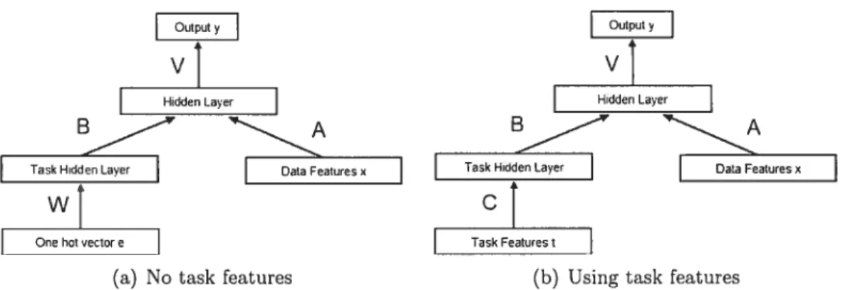
As mentioned in the introduction, the flrst techniques for modeling more than one task at the same time were developed in the context of multi-layer neural networks, which were modified so as to allow the process of inductive transfer (from one modeling task to another) to take place. We have developed a neural lletwork architecture that is based on such idea.s. The basic architecture of the fleurai network model, showil in Figures 3.la and 3.lb, has two hidden layers. The ftrst hidden layer is committed to processing task descriptors, in order to discover relationships between the tasks. The architecture assumes that such relations can be uncovered more easily when we perform a low-dimensioual embedding for task descriptors.
Otitput
vi
Hdden Layer
B
Task Hcdden Layer Data Featuresx
wI
One hot vector e
(a) No task features
Figure 3.1: Multi-task Neural Network architectures
In one version, shown in 3.la and in equation 3.1, we use as the input of the first layer a one-hot variable (a vector ek full of zeros except for a 1 at position k for coding symbol k) indicating the task number. The second layer receives the output of the first layer and the descriptors of the input x. Note that such an architecture does lot use any task descriptors except for an indicator of which task a specific
B A
20
input vector “belongs” to. Therefore, this architecture will learn an individual predictive model for each task, but the first layer will contain information about the relatedness of tasks with respect to the correlations in the mapping between input vectors and outputs (as this is the only way of learning any relatedness between tasks, in the absence of any other information). The precise mathematics for this model are:
P(y =
1Ix
,k) = sigmoid(Vtanh(Ax + B tanh(Wek)) (3.1)where ek is the one-hot variable defined above. The learned weights matrix W will
contain the low-dimensional embeddings for each task and will, in a sense, summa rize the relationships between the targets (their “position” in this low-dimensional space). In another version, shown in 3.lb and in equation 3.2, we use task descrip tors in the first layer as an aid for finding the relatedness of tasks. Here we learn an indirect predictive model for each task and the “positions” of the tasks in the low-dimensional embedding should be approximated better, given task descriptors that allow the algorithm to do so.
P(y = 1Ix ,tk) sigmoid(Vtanh(AX + B tanh(Ctk))) (3.2)
The parameters of the neural network (V, A, B, W) or (V, A, B, C) will be tuned by stochastic gradient ascent [12, 62] on the average log-likelihood of the training set (average of the logarithm of the above probabilities). Details of the learning procedure eau be found in Section 4.1.4.
Among the reasons for choosing this algorithm are the easiness of interpretation of the models, the speed of training and testing and its ubiquitousness in the computational chemistry community. We also feit that it would provide for a good baseline.
The algorithm can be applied to our computational chemistry setting as is, without further modifications. The task descriptors correspond to the biological target deseriptors and the input veetors are the molecular eompounds features.
21 3.3 An input-task similarity measure
We have mentiolled a couple of times the notion of similarity between tasks (through their “position” in a low-dimensional space, for instance). It would be interesting to formalize this notion and to put it to use in a framework that would learn relationships between the inputs+task descriptors and the oritputs in a sta tistically consistent way.
One way of doillg that is through the use of kernels. These are nothing but predefined similarity measures which, under fairly general assumptions, can be used to train very efficient learning algorithms that discriminate between patterns. R is easy to sec that we have two types of similarities that we cari use in our setting: a similarity measure between input vectors (molecular compounds) and one between tasks (biological protein targets). A learning algorithm that generalizes across tasks lias to somehow combine the two similarities in order to compute a more general measure of similarity, that between input-task pairs. In the case of MT
NNet, this is donc in the second hidden layer, where the shared representation of tasks (their representation in the low-dimensional embedding) is combined with the representation of the input features.
This measure of similarity, the input-task kernet, can be of the type used in Support Vector Machine algorithms [65]—i.e. it can be a non-linear function of inputs and task descriptors and cari project these into a higli-dimensional space. Typically, algorithms that learn relationships between inprit-task pairs and outputs using this kernel measure will find a separating hyperpiane in the resulting high dimensional space. This hyperplane will separate in some non-linear way in the input space the examples from the two classes.
Let us formalize the intuitions behind the idea of an input-task similarity mea sure. We try to find a map ‘I’ that takes pairs (x,t) into 1’(x,t) R’, where t is the vector of task features and x is the vector of inpllts, for a given mpllt-task pair (with D being the—possibly infinite—dimension of the resrdting combined space). Such a map would allow us to compute similarities between pairs of inputs/tasks
22 alld would allow us to generalize across both task features and input features at the same time.
Let Tbe the set of tasks, 15e the set of inputs and the map 5e Iî : IxT —* RD,
which gives a D-dimensional feature vector for each input-tasks pair. Our goal is then to choose a function, which should be optimal in some sense, from the set of functions F, which are linear in ‘I’, i.e.,
F(x,t; w) = ‘I’(x, t)tw (3.3)
(where is the transpose). This function would encode (in a linear fashion) the relationship between the input-task pair features and, combined with the respective outputs, will be tuned to fit some optimality criteria on the trailling set.
Note that IJ(x,t) from equation 3.3 is riot computed directly (for reasons that will become clearer shortly) and that our algorithm is only using dot-products in the feature space defined by ‘I’. The dot product between the application of I’ on two pairs is referred to as a kernet. More precisely, for two given pairs (x,tk)
and (x,ttm), we define the kernel as K((x, tk), (x, ttm)) and it is a function that computes the similarity between these pairs. We will see shortly how to compute this measure efficiently.
As shown by Crammer and Singer [20] and Sch51kopf and Smola
[651,
one eau rewrite equation 3.3 as follows, thanks to the Representer Theorem:= ci(xm,tm)K((X,tj, (x,tm)) (3.4)
(x;,t”)
where ci(xm,tm) is a vector of coefficients for each input-task pair from the training
set. The way to compute these coefficients such that they minimize some loss functional is what sets apart different learning algorithms that use kernels. Thus if we can evaluate efficiently the kernel, then we do not need to explicitly compute the feature vectors given Sy “I’. This is important because the computation of Jt
23
practice we choose not ‘1 but the kernel K, and for many choices of interest for K,
the corresponding I is infinite-dimensional. The ollly constraint on the choice of
K is that it must be positive semi-definite1.
Now we must define this general similarity measure. We take a bottom-up approach, by first defining similarity measures between pairs of tasks, then between pairs of inpllts, and then combining the two measures into a kernel function of the desired type. Thus, we eau use the following (non-exhaustive) list of kernels:
1. an identity kerilel K, which returns one if the two tasks have the same feature vector and zero otherwise (this forces the Gram matrix to be of the required type),
2. a Gaussian kerilel 1(tk,ttm) exp
(—
IItjII), with u2 being a tunablehyper-parameter.
3. a correlation kernel which computes the Pearson correlation coefficient, which is a dot-product betweell the normalized output vectors (y’ and ym)
corresponding to each tasks (over the inputs that are shared by the two targets). The Gram matrix corresponding to this similarity measure is not however positive semi-definite, and one way of making it positive semi-definite is by defining the following kernel:
4. a quadratic kernel K, which is . 1C (it has the necessary property of
aiways being positive semi-definite).
We can define in a similar way ,, K, and 1Cr, the kernels for the input
features. So far, we have not mentioned a way of combilling the kernels. If we were to deal only with task features (or only with the input features), combining the kernels could be done by simple addition, possibly also via a weighted sum, since
‘It means that for any finite set P of input-task pairs s, the Gram matrix G associated with
P must flot have any negative eigenvalues. The entry (i,j) of G is = K(s,s) with s e P
24 the weighted sum of positive semi-definite matrices is also positive semi-definite:
(3.5)
We can do exactïy the same for the kernel of the input features:
(3.6)
If we are interestedin combining )C’r and , so that we can compute the simi
larity between input-task pairs, we could use the tensor product to get K((x,tk), (x, ttm)).
Intuitively, two given pairs should be most similar if and only if ttm) is at its maximum and Ki(x,x) is at its maximum, too. We cannot for any practical purpose, compute the tensor product (because of the infinite dimension vectors), but it turns out that the product is equivalent [65] to
K((x,tj, (x,tm)) — 1C(tk,tm) (3.7)
which is a handy shortcut that also follows our intuitions!
Given this kernel and the definition of the F function that is to 5e learned (from equation 3.4), we can now move on to defining learning algorithms that could use these and the outputs y in order to learn a way to discriminate between input-task pairs.
3.4 JRarik
The first such algorithm that we will consider is called JRank. It was proposed by Basilico and Hofmann [5] and it was the first to use the above idea of unifying task and input features into a common framework, albeit in a different problem setting, where the tasks corresponded to people and inputs corresponds to items that people rated (so a combination of content-based and collaborative filtering).
25 tron [61], which means that it has several useful characteristics such as its simplicity and its onhine nature. It is a kernel-based extension of the original perceptron ai gorithm; such an extension is typically referred to as the kernet perceptron [31].
The essence of the algorithm is a.s follows. We are interested in performing or dinal TegTession, that is we would be interested in learning an ordinal value for each input. This contrasts to the more common regression and classification problems in that the numerical value of the output is not important. What is important is the order that we define on the outputs.
In order to represent this intuition in a mathematical way, the output of the function F is binned via a set of adaptive thresholds O
e
Rk, where k is the number of “output levels” (ordinal values) we are interested in (Ok = +oo for convenience).This is done in order to predict the output level from an input-task pair: by simply selecting the number of the bin where F(x,t; w) falls into. The prediction ftmction f(x,t; w,O) depends straightforwardly on O: it outputs a level i associated with the interval [O,Oi+1) which contains F(x,t;w).
On a more fundamental level, what JRank is doing is finding a set of k hy perplanes in the feature space defined by ‘P. The space defined by two adjoining hyperpianes corresponds to a given “output level” (ordinal value). JRank will find this set by moving along the gradient of the loss functional and finding a local optimum.
The framework of ordinal regression is appropriate for both binary classification problems—where we would interpret the two output levels as “high” and “low”— and for multi-class
/
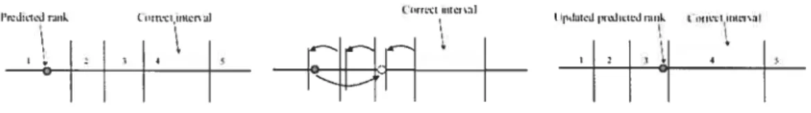
regression problems, where the transformation of the numerical values to an ordinal scale poses no problem.Algorithm 1, as described in [5], is a straightforward extension to the kernel per ceptron algorithm [31]. As in [20], JRank projects cadi instance from our dataset onto the real line. Each ranking is tien associated with a distinct sub-interval of the reals. During learning these sub-intervals are updated: if and when tic current set of parameters predicts an incorrect sub-interval, the parameters are updated such that the new predicted rank is doser to the sub-interval (and vice-versa, by
26
Mgorithm 1 JRank
1: {c is a sparse parameter matrix, one element per experimental observation}
2: {A(,t) is the output level corresponding to input x and task t}
3: (x,t) = O,VA(x,t)
4: {O is a vector of thresholds, defining the bins for the ordinal values} 5: O=O,Vi=1,...,k—1andOk=+oo
6: {N is the number of iterations}
7: for n 1 to do
8: for ail A(x,t) do
9: {The estimated activity level (equation 3.3)}
10: â=f(x,t;a,O)
11: {If the estimated activity level is incorrect, we update the parameters}
12: if â > A(x,t) then
13: {Following the gradient}
14: (x,t) = (x,t) + a —A(,t)
15: {The value of the F function becomes doser to the correct bin}
16: fori=A(,)toâ—1 do
17:
18: end for
19: else if â < A(,t) therr
20: {Following the gradient}
21: (x,t) (x,t) + a — A(xt)
22: {The value of the F function becomes doser to the correct bin} 23: for i â to A(,t) — 1 do 24: OOl 25: end for 26: end if 27: end for 28: erid for
27 modifying the boundaries of the sub-intervals).
A(,t) is the output level observed for the pair (x,t) (the ys, essentially). In
the formulation it is also understood that we have access to the set of ail the data triplets (x,t, A(,t)). Before learning, the sparse parameter matrix c has non-zero
entries c(X,t) only for the observed pairs (x,t). It cari he used for prediction via
equation 3.4. A set of threshokls/hins O (one per ordinal value) is also learned. The algorithrn runs through the dataset in stages/iterations, updates Ù(x,t)
and updates the thresholds if it predicts an incorrect activity level. The algorithm assumes that the ranks are ordered from j = 1 to k, but it cari be easily modifted
to accommodate other types of ranks.
The updates of a(x,) follow the prediction error (the difference between the
predicted rank and the actual rank, also called the ranking toss), i.e., they follow the gradient, while the thresholds O are updated so that the value of the F function hecomes doser to the correct bin at the next iteration. This is illustrated in Figure 3.2 (taken from [20]).
Ire,I:ci%-d rani Ct,LetnL,ç
(0rrLt,0e,a
1,d:urcd ‘Tcict2d r-an ton,cc(nin:rsaI
I
ç ç 2 1 4
Figure 3.2: Intuition behind the update rule of JRank
The algorithm has two hyper-parameters:
1. The width of the Gaussian kernel . Ideally, there should be one for each
(task and input) kernel. 2. The number of iterations
It is worth noting that the algorithm functions correctly and as expected when k = 2, i.e., it learns to perform hinary classification. The algorithm reduces to
28 simple single-task learning if the dataset has only one target (a becomes a vector)— which is quite handy because it allows us to compare directly single-task learning ($T-JRank) with multi-task learning (MT-JRank).
In its most general form, the algorithm needs output levels in order to learn. This is a desirable feature, since very often in a computational chemistry context we are interested in learning different activity tevets. Thus given a compound and a target, the compound can 5e ttinactive) “somewhat active”, “quite active”, “defi nitely active”, for instance. JRank would thus accommodate easily such scenarios. The algorithm’s runtime is quadratic in the size of the training set. This is because the computation of the prediction function involves an iteration through the entire set, in order to compute the similarity between the currellt input-task pair and the rest of the pairs in the training set. These computatioll can be cached (since they do not lleed to be recomputed at each iteration), but this quickly 5e-comes intractable as the number of input-task pairs grows above 10000 (our dataset is much larger than that). Needless to say, computing the Pearson’s correlatioll coefficient is computationally very expensive, as it adds a factor of M (the number of input vectors in the dataset, approximately 16000 in our case) each time one computes the similarity between tasks.
As is the case with MT-NNet, JRank can 5e adapted straightforwardly to our problem setting. $ince our are essentially binary values, the runtime of the algorithm will be reduced.
3.5 Multi-Task Support Vector Machines 3
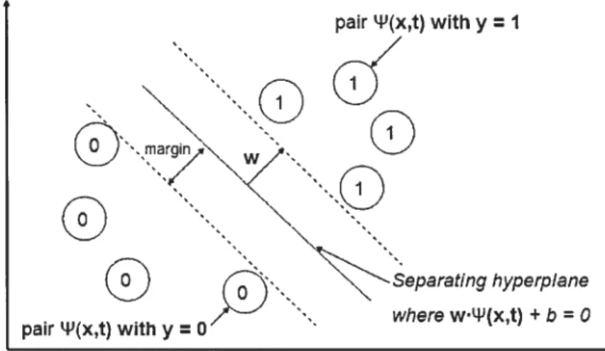
The general idea behind JRank—to find a hyperpiane that separates two classes— can 5e taken further by stipulating that this hyperplane shoild 5e as far as possible from the two different classes, in the feature space defilled by LIJ. Assume, as shown in Figure 3.3, that we have managed to filld a candidate hyperpiane that separates the two classes sllch that the distance from it to the closest input-task pairs from
29
either class is the same. Then it can be shown [70] that for the decision function specified by this hyperpiane there will be an upper bound on the generalizatio performance, which depends on the margin obtained with it.
pair W(x,t) with y I
hyperpiane
where w’.Pfx,t) +b =Q
Figure 3.3: Intuition behind the Multi-task Support Vector Machine approach
JRank, as desribed above, will not generally find this hyperpiane, because the objective function is non-convex. There is however an algorithm that can efficiently find this hyperpiane and its generic name is the Support Vector Machines (SVMs; the “support vectors” are those transformed data that are closest to the optimal hyperpiane). Because we are using this algorithm to find separating hyperpianes in joint feature spaces of inputs and tasks, we eau our version the “Multi-Task Support Vector Machine”.
Let us formalize the intuitions. As above, we are interested in a linear separator, therefore we are looking for a weight vector w that minimizes some loss, that in turn uses the following decision function:
f(x,tk;c) _ b+wt.(x,tj b+
L(x,tm) (x,tk)t. (x,tm) (3.8)
(x,y,t’)
o
pair(x,t) withy
30 vector w) in a non-linear transformation of the feature space. To do so, we re-write equation 3.4 into the following decision function:
f(x,tk; c) b+wt.TJ(x,tk) =
y2 K((x,tk), (x,tm))+b
(x,y,t”)
(3.9) These are the so-called dual representation of $VMs. We can see that, as in the JRank case, in these decision functions, data appear ollly in the form of kernels evaluated at pairs of data-points or dot-products of data pairs (a dot-produet is a linear kernel, as well).
The basic idea of the Support Vector Machine algorithm is that the procedure for choosing the parameter matrix i is one that gives rise to a hyperpiarie that
lias a special property: it maximizes the margin between it and the data from the two classes (so this is the “loss function” that it tries to minirnize). The actual equation
/
objective function that is to 5e millimized is [65]:— x,t(Xtm)YYA((,tk), (x.tm))
(xT,y,t”) (x ,y,tk),(x,“,t”)
(3.10) subject to c(x ,trn) O and Z(x;”,y,t’”) ci(x,trn) = 0. This is a quadratic opti
mization problem: it is convex anci it can 5e solved in polynomial time. Schblkopf and Smola [65] provide several algorithms for doing so efficiently.
The separating hyperpiane might not be able to perform a perfect separa tion, i.e. without mislabeling any training examples, even in a non-linear high dimensional space. Moreover, even if the separation is perfect, it could suifer from the problem of overfttting—the hyperpiane could 5e very close to the data and the solution found hy it would therefore have a poor Sound on the generation error. One coulci thus introduce some slack variables that allow for separating hyperplanes that allow for mislabeled training examples. These variables can 5e summarized mto a single constraint that introcluces a trade-oif between the margin of the sepa ration and the number of mislabeled examples. This constraint is a box-constraint
31 on û: O C, with C being the so-called soft-margin parameter that
controls the trade-oft just described.
As we mentioned before, the mai11 difference between JRank and MT-$VM is
that the training procedure for MT-SVM produces a maximum-margin separating hyperpiane, which is, under the assumption that a maximum-margin is desirable, the best-case scenario of JRank. JRank is however faster and should in theory produce solutions that are close to the MT-SVIi solution (especially when nsed with non-linear kernels).
The algorithm just presented is the standard description of the Support Vector Machines. It uses the custom kernels that unify the inputs and tasks into one joint feature space in which we can compute efficiently similarities between input-task pairs. There are many more details of the implementation that we glossed over, but they are standard issues that arise when using the standard SVM algorithm. We used an off-the-shelf implementation of the algorithm—
[421
provides extensive details about it.We mentioned that this is a quadratic optimization problem (i.e. the criterion to be minimized is a polynomial of degree 2 in the parameters). Depending on the implernentation aiid on the data, the complexity is somewhere between cubic and quadratic in the number of input-task pairs. The algorithm is also linear in the size of the training set at the testing stage: in order to classify an input-task pair into either of the classes, we need to compute the similarity of the pair with ail the rest of the pairs from the training set (JRank suffers from the same problem).
The choice of kernels is the same as with JRank and for the same reasons. As described above, MT-SVM will not be able to perform ordinal regression. One could extend the training procedure in order to perform muiti-ciass classification (in a one vs. ail setting), but this would be oniy a very rough approximation to the idea on ordinal regression. The ability to do the iatter is one of the advantages of JRank.
MT-SVM can be readily applied to the computational chemistry dataset. Es sentially, one only needs to write a wrapper function that computes the similarity
32 measure between input-task pairs and the resuit will 5e a decision function that will separate in an optimal wa.y active and inactive molecules in the joint molecule target feature space.
3.6 Partial Least Squares
Partial Least Squares (PLS) is a very popular algorithm in the computational chemistry research comrnunity, partly because it is easy to implement and because it serves as a baseline for comparison. It combiies some techniques from Principal Component Analysis with ones from ordinary linear regression. If we assume that we have access to a matrix of inputs X and (in the most general case) a matrix of corresponding desired outputs Y (in our case, since there’s only one output per input, this will 5e a vector) then the goal of PLS will he to find a set of latent components that performs a decomposition of both X and Y such that these components explain most of the covariance between X and Y.
We have only used PLS for single-task prediction problems, therefore we do not provide more deta,ils of it in this thesis. Wold et al [72] show however its inner workings in more detail.
CHAPTER 4
EXPERIMENTS
In this chapter, we describe the experiments that we performed using the algo rithms from Chapter 3
4.1 Experimerrtal Setup
First we provide a technical description of the dataset that we used, a.s well as most of the details related to our experimental setup and resuits. Because of the proprietary nature of the dataset, it is not possible for us to give alt the details needed for reproducing our resuits.
4.1.1 Datasets arid Descriptors
Ail the liga.nds (molecular compounds) used in this study were in the posses
sion of AstraZeneca R&D Montreal. They ail sa.tisfy the Lipinski mie of flue’ [51]. Different subsets of these moiecules have been screened against 24 biological tar gets. The screens have been made at different times, with some small variations in protocol. Our dataset is thus a collection of disparate HTS campaigns brought together for this study. Figure 4.1 shows the number of compounds for which the screening data was available for each target. We detailed the active and inactive compounds.
The compounds descriptors were cornputed with MOE (version 2004.03) [17] for each of the molecular compotmds2. The set of 469 descriptors range from atom frequencies [11, 56] and topologicai indices [3, 35,44, 58] to 3D surface area descrip tors. We also computed MACC$ [25], Randic [59] a.nd EState [36] descriptors that
1A set of rues of thumb that indicate whether a molecule is likely to be active or flot 2A forthcorning technical report will give more details about the procedure. This report will be written by the computational chemistry specialists that constructed the dataset and will be available for download from the webpage of our laboratory, www.iro.umontreal.ca/lisa