arXiv:1710.06321v1 [astro-ph.EP] 17 Oct 2017
October 18, 2017
The discovery of WASP-151b, WASP-153b, WASP-156b: Insights on
giant planet migration and the upper boundary of the Neptunian
desert
Olivier. D. S. Demangeon
1,⋆, F. Faedi
2,9, G. Hébrard
3,4, D. J. A. Brown
2, S. C. C. Barros
1, A. P. Doyle
2, P. F. L.
Maxted
12, A. Collier Cameron
7, K. L. Hay
7, J. Alikakos
18, D. R. Anderson
12, D. J. Armstrong
2,6, P. Boumis
18, A. S.
Bonomo
8, F. Bouchy
5, C. A. Haswell
17, C. Hellier
12, F. Kiefer
3, K. W. F. Lam
2, L. Mancini
19,16,8, J. McCormac
2, A. J.
Norton
17, H. P. Osborn
2, E. Palle
14,15, F. Pepe
5, D. L. Pollacco
2, J. Prieto-Arranz
14,15, D. Queloz
10,5, D. Ségransan
5, B.
Smalley
12, A. H. M. J. Triaud
11,13, S. Udry
5, R. West
2, and P.J. Wheatley
21 Instituto de Astrofísica e Ciências do Espaço, Universidade do Porto, CAUP, Rua das Estrelas, 4150-762 Porto, Portugal 2 University of Warwick, Department of Physics, Gibbet Hill Road, Coventry, CV4 7AL, UK
3 Institut d’Astrophysique de Paris, UMR7095 CNRS, Université Pierre & Marie Curie, 98 bis boulevard Arago, 75014 Paris, France 4 Observatoire de Haute-Provence, Université d’Aix-Marseille & CNRS, 04870 Saint Michel l’Observatoire, France
5 Observatoire de Genève, Université de Genève, 51 Chemin des Maillettes, CH-1290 Sauverny, Switzerland 6 Astrophysics Research Centre, Queen’s University Belfast, University Road, Belfast BT7 1NN, UK
7 Centre for Exoplanet Science, SUPA, School of Physics and Astronomy, University of St Andrews, St Andrews, KY16 9SS, UK 8 INAF - Osservatorio Astrofisico di Torino, Via Osservatorio 20, 10025 Pino Torinese, Italy
9 INAF - Osservatorio Astrofisico di Catania, Via S. Sofia 78, I-95123 Catania, Italy 10 Cavendish Laboratory, JJ Thompson Avenue, CB3 0HE, Cambridge, UK
11 Institute of Astronomy, Madingley Road, CB3 0HA, Cambridge, UK 12 Astrophysics Group, Keele University, Staffordshire, ST5 5BG, UK
13 School of Physics & Astronomy, University of Birmingham, Edgbaston, Birmingham, B15 2TT, UK 14 Instituto de Astrosfísica de Canarias (IAC), 38205 La Laguna, Tenerife, Spain
15 Departamento de Astrofísica, Universidad de La Laguna (ULL), 38206 La laguna, Tenerife, Spain 16 Max Planck Institue for Astronomy, Königstuhl 17, 69117 Heidelberg, Germany
17 School of Physical Sciences, The Open University, Milton Keynes, MK7 6 AA, UK
18 Institute for Astronomy, Astrophysics, Space Applications and Remote Sensing, National Observatory of Athens, 15236 Penteli,
Greece
19 Department of Physics, University of Rome Tor Vergata, Via della Ricerca Scientifica 1, 00133 Roma, Italy
Received date / Accepted date
ABSTRACT
To investigate the origin of the features discovered in the exoplanet population, the knowledge of exoplanets’ mass and radius with a good precision (. 10 %) is essential. To achieve this purpose the discovery of transiting exoplanets around bright stars is of prime interest. In this paper, we report the discovery of three transiting exoplanets by the SuperWASP survey and the SOPHIE spectrograph with mass and radius determined with a precision better than 15 %. WASP-151b and WASP-153b are two hot Saturns with masses, radii, densities and equilibrium temperatures of 0.31+0.04
−0.03MJ, 1.13 +0.03 −0.03RJ, 0.22 +0.03 −0.02ρJand 1, 290 +20 −10K, and 0.39 +0.02 −0.02MJ, 1.55 +0.10 −0.08RJ, 0.11+0.02 −0.02ρJand 1, 700 +40
−40K, respectively. Their host stars are early G type stars (with magV ∼ 13) and their orbital periods are 4.53
and 3.33 days, respectively. WASP-156b is a Super-Neptune orbiting a K type star (magV = 11.6) . It has a mass of 0.128+0.010 −0.009MJ, a radius of 0.51+0.02 −0.02RJ, a density of 1.0 +0.1 −0.1ρJ, an equilibrium temperature of 970 +30
−20K and an orbital period of 3.83 days. The radius
of WASP-151b appears to be only slightly inflated, while WASP-153b presents a significant radius anomaly compared to the model ofBaraffe et al.(2008). WASP-156b, being one of the few well characterised Super-Neptunes, will help to constrain the still debated formation of Neptune size planets and the transition between gas and ice giants. The estimates of the age of these three stars confirms an already observed tendency for some stars to have gyrochronological ages significantly lower than their isochronal ages. We propose that high eccentricity migration could partially explain this behaviour for stars hosting a short period planet. Finally, these three planets also lie close to (WASP-151b and WASP-153b) or below (WASP-156b) the upper boundary of the Neptunian desert. Their characteristics support that the ultra-violet irradiation plays an important role in this depletion of planets observed in the exoplanet population.
Key words. Planetary and satellites: detection – Stars: individual: WASP-151, WASP-153, WASP-156 – Techniques: radial
1. Introduction
The successful harvest of exoplanets (see for example exo-planet.eu, Schneider et al. 2011) during the last two decades completely metamorphosed the field of exoplanet science. The initial assumption that the solar system was a typical example of planetary systems is long gone (as stated by
Mayor & Queloz 2012). The Kepler mission (Borucki et al.
2010) delivered 4,496 transiting planetary candidates, includ-ing 2,248 confirmed planets (accordinclud-ing to the NASA Exoplanet Archive, http://exoplanetarchive.ipac.caltech.edu/,
August 2017). This sample revealed various features of the exoplanet population demonstrating the necessity of a very large sample to encompass the exoplanets’ diversity (see
Borucki 2017, for a recent review). One of many surprising
results from Kepler is that the orbital distance of exoplan-ets appears to be nearly random regardless of their size (e.g.
Fabrycky et al. 2014). One striking exception to this
observa-tion is the so called sub-jovian desert or short period Neptu-nian desert (e.g Mazeh et al. 2016; Matsakos & Königl 2016;
Kurokawa & Nakamoto 2014; Szabó & Kiss 2011). It corre-sponds to a depletion of planets at short orbital periods (P < 10 days) with masses or radius between super-Earth and sub-jovian planets (see Fig 10). One possible explanation for this desert is the strong irradiation (bolometric and in particular ex-treme ultra-violet) from the parent star at those short orbital distances, especially at the early stages of the star’s life. The strong stellar irradiation might have striped away the atmosphere of sub-jovian planets which had quickly migrated to the vicin-ity of their parent star and were not massive enough to re-tain their atmosphere, only leaving a super-Earth size core (e.g.
Lundkvist et al. 2016;Lecavelier Des Etangs 2007). The
mech-anism responsible for the presence of giant planets in the vicin-ity of their parent star is still debated. However, the discovery by David et al.(2016) of a Super-Neptune size planet orbiting close to a 5-10 Myr old star suggests that high eccentricity mi-gration (e.g.Rasio & Ford 1996;Fabrycky & Tremaine 2007) is unlikely for this system (the tidal circularisation happening at longer timescales) and only leaves disk migration (e.g.Lin et al.
1996; Ward 1997) and in-situ formation as possible scenarios.
Understanding the origin of the Neptunian desert could thus change our vision of gas and ice giant planet formation and evo-lution.
Unfortunately a large fraction of the planets discovered by Kepler surrounding the Neptunian desert don’t have an ac-curate (precision . 10 %1) determination of their mass and
radius due to the faintness of their parent star. In this con-text ground based transit photometry surveys like SuperWASP (Pollacco et al. 2006), targeting bright stars, are essential con-tributors. In this paper, we present the WASP and SOPHIE dis-covery of two hot Saturns and one warm super Neptune, with mass and radius measured with a precision better than 15 %, and discuss their impact on the formation and evolution theories of ice and gas giants. In Section2, we describe the photometric and radial velocity observations acquired on the three systems. In Section3, we present our analysis of the data with the resulting stellar and planetary parameters. Finally in Section4, we discuss the nature and composition of these planets and their impact on
⋆ e-mail: olivier.demangeon@astro.up.pt
1 The exact precision required is difficult to assess, but a precision
of 20 to 30 % on the planetary density is usually required to be able to discriminate between the main families of planets (see for exam-ple Benz et al. 2013;Grasset et al. 2009). This correspond to an un-certainty on the radius of roughly 10 %.
planet formation and evolution theory with a focus on the migra-tion of the hot giant planet populamigra-tion and the upper boundary of the Neptunian desert.
2. Observations
2.1. Discovery: WASP
The Wide Angle Search for Planets (WASP) operates two robotic telescope arrays, each consisting of eight Canon 200m, f/1.8 lenses with e2v 2048 × 2048, Peltier-cooled CCDs, giv-ing a field of view of 7.8 × 7.8 degrees and a pixel scale of 13.7′′(Pollacco et al. 2006). SuperWASP is located at the Roque do los Muchachos Observatory on La Palma (ORM - ING, Canary Islands, Spain), while WASP-South is located at the South African Astronomical Observatory (SAAO - Sutherland, South Africa). Each array observes up to eight pointings per night with a typical cadence of 8 min and an exposure time of 30 seconds, with each pointing being followed for roughly five months per observing season. In January 2009, SuperWASP re-ceived a significant system upgrade that improved our control of red noise sources such as temperature-dependent focus changes (Barros et al. 2011;Faedi et al. 2011), leading to substantially improved data quality.
All WASP data are processed by the custom-built reduction pipeline described inPollacco et al. (2006), producing one light curve per observing season and camera. These light curves are passed through the SysRem (Tamuz, Mazeh, & Zucker 2005) and TFA (Kovács, Bakos, & Noyes 2005) de-trending algo-rithms to reduce the effect of known systematic signals, be-fore a search for candidate transit signals is performed us-ing a custom implementation of the Box Least-Squares algo-rithm (BLS; Kovács, Zucker & Mazeh 2002), as described in
Collier Cameron et al. (2006, 2007). Once candidate planets
have been identified, a series of multi-season, multi-camera anal-yses are carried out to confirm the detection and improve upon initial estimates of the candidates’ physical and orbital param-eters, which are derived from the WASP data in conjunction with publicly available catalogues (e.g. UCAC4,Zacharias et al. 2013; 2MASS,Skrutskie et al. 2006). These additional analyses are essential for rejection of false positives, and for identification of the best candidates. This process allowed to detect three tran-sit planets that we will now introduce.
1SWASPJ231615.22+001824.5 (2MASS23161522+0018242),
hereafter WASP-151, lies very close to the celestial equator and is thus visible to both WASP arrays. A total of 45, 945 data were obtained between 2008-06-12 and 2012-11-28, 16, 375 from SuperWASP and 29, 570 by WASP-South. A search for periodic modulation in the WASP light curves, such as might be caused by stellar activity or rotation, was carried out using the method ofMaxted et al. (2011). No significant periodicity was identified, and we place an upper limit of 2 mmag on the amplitude of any modulation. During these observations a total of 195 transits were covered of which 27 were full or quasi-full events. The WASP data show a periodic reduction in stellar brightness of approximately 0.01 mag, with a period of roughly 4.5 days, a duration of approximately 3.7 hours, and a shape indicative of a planetary transit. The WASP thumbnails of WASP-151 show some contamination from a background galaxy about 20" from the target and thus within our first aperture. The galaxy is about 3 magnitude fainter in V than our target. We calculated a dilution factor for WASP-151 of about 1% and thus negligible when considering WASP data.
1SWASPJ183702.97+400107.4 (2MASS18370297+4001073), hereafter WASP-153, is our second transiting planet host. 42, 349 photometric measurements were made by SuperWASP between 2004-05-14 and 2010-08-24, with no observations by WASP-South owing to the high declination of the target (+40o). We found no significant periodic modulation, and we place an upper limit of 1.5 mmag on the amplitude of any such light curve variation. There are a total of 688 transits observed of which 54 are good events2. Our BLS searches identified the
signature of a candidate transiting planet on a 3.3 days orbit, in the form of a periodic 0.006 mag, 3 hours reduction in stellar brightness.
1SWASPJ021107.61+022504.8 (2MASS02110763+0225050),
hereafter WASP-156, is our third and last transiting planet host. We again found no significant periodic modulation, and we place an upper limit of 1 mmag on the amplitude of any such light curve variation. As with WASP-151, the equatorial declination of WASP-156 allows both WASP arrays to monitor the star for flux variations. 22809 flux measurements were made, 13481 by SuperWASP and 9328 by WASP-South. A total of 230 transits were observed of which 23 are good events2. A 2.3 hours long, 0.007 mag reduction in brightness was found to repeat on a 3.8 days period with a typical planetary transit-like shape.
2.2. Photometric follow-up
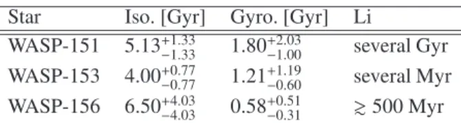
Table 1. Summary of the photometric observation of WASP-151, WASP-153 and WASP-156.
Date Instrument Filter Comment
WASP-151b
06/2008→11/2012 WASP Johnson R detection 03/09/2015 IAC80 Johnson R full transit 01/11/2015 IAC80 Johnson R full transit 15/06/2016 TRAPPIST Sloan z full transit 04/09/2016 EulerCam NGTS partial transit 24/10/2016 EulerCam NGTS full transit 12/2016→03/2017 K2 Kepler 13 full transits
WASP-153b
05/2004→08/2010 WASP Johnson R detection 17/07/2015 Liverpool Johnson R partial transit 05/08/2017 RISE-2 V+R full transit
WASP-156b
07/2008→12/2010 WASP Johnson R detection 29/12/2014 EulerCam Gunn z full transit 07/11/2016 EulerCam Gunn r full transit 27/12/2016 NITES Johnson I partial transit
2.2.1. Ground-based photometric follow-up observations The WASP consortium has access to multiple observing facili-ties that can be used to obtain additional in-transit photometric observations. These follow-up light curves are used to confirm the presence of the candidate signal, particularly useful in the case of unreliable initial ephemerides, and are also used to im-prove the accuracy of our light curve modelling, and to constrain the system parameters more precisely. A list of the follow-up photometric observations for our three planets is presented in Table1.
2 Good events refers to full transit observations which didn’t suffer
from obvious deformations due to the conditions of observation.
WASP-151b Two full transits of WASP-151 were observed on 2015-09-03 and 2015-11-01 with the CAMELOT camera of the 0.82 m ( f /11.3) IAC-80 telescope, which is operated on the island of Tenerife by the Instituto de Astrofísica de Canarias (IAC) at the Spanish Observatorio del Teide. CAMELOT has a 2048 × 2048 pixel CCD with a scale of 0.304′′pixel−1and a 10.6′field-of-view. Images were bias and flat-field corrected us-ing standard techniques.
An additional full transit was observed on 2016-06-15 with the robotic 0.6 m TRAnsiting Planets and PlanetesImals Small Telescope (TRAPPIST; Jehin et al. 2011; Gillon et al. 2011) at the La Silla Observatory operated by the European Southern Observatory (ESO). TRAPPIST is equipped with a thermoelectrically-cooled 2K × 2K CCD with a pixel scale of 0.65′′, giving a 22′× 22′field of view. A Sloan-z′filter was used for the transit observations of this system, during which the po-sitions of the stars on the chip were maintained to within a few pixels thanks to a software guiding system that regularly derives an astrometric solution for the most recently acquired image and sends pointing corrections to the mount if needed. After carrying out bias, dark, and flat-field corrections we extract stellar fluxes from our images using the IRAF3/DAOPHOT aperture
photom-etry software (Stetson 1987). Several sets of reduction param-eters were tested on stars of similar brightness to WASP-151, from which we selected the set giving the most precise photom-etry. After a careful selection of reference stars, the transit light curves were finally obtained using differential photometry.
The 1.2 m Swiss telescope using EulerCam (Lendl et al. 2012), also at La Silla, observed a full transit of WASP-151b on 2016-10-24 and a partial transit on 2016-10-24. In both cases, a filter with a central wavelength of 698 nm and an effective band-width of 312 nm was used; this filter is the same as that used by the Next Generation Transit Survey (NGTS;Wheatley et al. 2013,2014). The Swiss telescope employs an absolute tracking system which matches point sources in each image with a cata-logue and adjusts the telescope’s pointing between exposure to compensate for drift. In this manner, the pixel position of the star is maintained throughout. All data were reduced as outlined inLendl et al. (2012), and light curves were produced through differential aperture photometry. To minimise scatter in the light curves, we carefully selected the most stable field stars to use as references.
WASP-153b A partial transit of WASP-153b was observed on 2015-07-17 in the Johnson-R filter using the RISE instrument mounted on the robotic Liverpool Telescope (LT; Steele et al. 2004) at ORM. RISE is equipped with a back-illuminated, frame-transfer, 1024 × 1024 pixel CCD. Images were automat-ically bias, dark, and flat-field corrected by the standard RISE reduction pipeline, which uses standard IRAF routines.
A full transit was later obtained with RISE-2 mounted on the 2.3 m telescope situated at Helmos observatory in Greece on 2017 August 5. The CCD size is 1K × 1K with a pixel scale of 0.51′′ and a field of view of 9′× 9′ (Boumis et al. 2010). The exposure time was 12 s and the V+R filter was used. As for the previous transit observation, the images were processed standard RISE reduction pipeline.
3 IRAF is distributed by the National Optical Astronomy
Observato-ries, which are operated by the Association of Universities for Research in Astronomy, Inc., under cooperative agreement with the National Sci-enceFoundation.
WASP-156b A partial transit of WASP-156b was observed in the Johnson-I filter on 2016-12-27 using the Near Infra-red Tran-siting ExoplanetS (NITES) Telescope (McCormac et al. 2014), located at ORM. NITES is a semi-robotic, 0.4 m ( f /10) Meade LX200GPS Schmidt-Cassegrain telescope, mounted with a Fin-ger Lakes Instrumentation Proline 4710 camera and a 1024 × 1024 pixel deep-depleted CCD made by e2v. The telescope has a field of view of 11 × 11′ squared, and a pixel scale of 0.66′′pixel−1. Autoguiding is performed using the DONUTS algorithm (McCormac et al. 2013). After performing bias and flat-field corrections using PyRAF4 and the standard routines
in IRAF, aperture photometry was performed using DAOPHOT and multiple comparison stars, selected to minimise the RMS scatter in the out-of-transit light curve.
In addition to the NITES observations, EulerCam was used to observe two full transits of WASP-156b, on 2014-12-29 us-ing a Gunn-z filter and on 2016-11-07 usus-ing a Gunn-r filter. The 2014 observations, however, are unreliable owing to large PSF variations, and stellar counts in the non-linear regime of the Eu-lerCam CCD.
2.2.2. K2 observations of WASP-151
In addition to the ground-based photometric observa-tions described in the previous secobserva-tions, WASP-151 (alias EPIC 246441449) was observed by NASA’s Kepler Space Tele-scope in its two-reaction wheel mission K2 (Howell et al. 2014) during Campaign 12. The observations span over ∼ 79 days (from 15th December 2016 to 4th March 2017) apart from 5 days (from 1st February 2017 to 6th February 2017) when the spacecraft was in safe mode.
Since Campaign 9, the K2 consortium releases the raw ca-dence data shortly after downlink from the Kepler satellite. These data are raw, as opposed to the science cadence data like the target pixel files (tpf), for two main reasons5. First their
for-mat, the raw cadence data are provided as one file per cadence delivering the pixel counts for the whole focal plane as a table. In order to construct the image time series of a target, we need the pixel mapping reference file which specifies the (column, row) CCD coordinates for each value in the raw cadence data tables. Second, the raw cadence data are not calibrated. It means that they are not reduced with the Kepler pipeline (Quintana et al. 2010) and thus not corrected for background, dark, smearing trails, undershoot or non-linearity of the pixels response. The formatting and calibration of the raw cadence data for all the tar-gets of a K2 campaign is a very lengthy procedure and even if the raw cadence data for Campaign 12 have been released sev-eral months ago, the calibrated tpf are, at this moment, still un-available. Therefore, to be able to benefit from the high quality light-curves of the WASP-151 system provided by the K2 mis-sion, we decided to format and reduce ourselves the raw cadence data.
To obtain an image time series, we used the Kadenza6
soft-ware (Barentsen 2017) provided by the NASA’s Kepler/K2 Guest Observer Office. Then, to extract the light-curve, we used 4 PyRAF is a product of the Space Telescope Science Institute, which
is operated by AURA for NASA.
5 For more details on the Kepler raw and science cadence data, we refer
the reader to the technical note entitled Format Information for Cadence Pixel Files available at https://archive.stsci.edu/k2/manuals/KADN-26315.pdf
6 The Kadenza software is available on GitHub at
https://github.com/KeplerGO/kadenza or on Zenodo at
https://doi.org/10.5281/zenodo.344973
the Polar software (Barros et al. 2016) which performs a partial calibration by subtracting the background and dark values thanks to estimates obtained on the images themselves. In parallel to the Polarreduction, we also reduced the image time series with the Python package Everest (Luger et al. 2016) to check the scien-tific validity of our reduction. Everest has been recently used to extract the light-curve of the TRAPPIST-1 system observed by K2 during the same campaign (Luger et al. 2017) and thus in the same conditions. The two light-curves are almost identical and compatible at 1 sigma giving us confidence in the scientific quality of our data reduction.
The light-curve clearly display transit features at the ephemeris inferred from the WASP data with no sign of out-of-transit variations. A search for periodic modulation caused by stellar activity showed a tentative detection with an amplitude of 1 ppt (∼ 1 mmag) at a period of 35 days. We then searched the light-curve for additional transit features (apart from WASP-151b’s transit). We investigated a tentative mono transit-shaped feature which proved to be an artifact due to the position-flux decorrelation technique used by Polar. For this decorrelation, we cut the K2 image time-series in several parts where the be-havior of the pointing jitter of the Kepler satellite can be safely assumed to be 1 dimensional (for more details seeBarros et al. 2016). The mono transit-shaped feature was appearing precisely at the junction of two of those parts. A slight change of the loca-tion of the cut made the feature disappear. Finally, no addiloca-tional transit features was detected.
For the analysis, we only kept intervals of 2 times the tran-sit duration before and after each trantran-sit of WASP-151b. The phase-folded Polar-K2 light-curve of WASP-151 is shown in the bottom panel of Fig2.
2.3. Spectroscopic follow-up
The spectroscopic follow-up of these three candidates was mainly performed with SOPHIE, the spectrograph dedicated to high-precision radial velocity measurements at the 1.93-m tele-scope of the Haute-Provence Observatory, France (Bouchy et al. 2009). For two systems, it was also complemented by radial ve-locities obtained with the CORALIE spectrograph at the 1.2-m Euler-Swiss telescope at La Silla (Queloz et al. 2000), Chile. The first goal of these spectroscopic observations is to establish the planetary nature of the transiting candidates found in pho-tometry (see Section2.3.2) The second goal is to characterize the secured planets by measuring in particular their masses and orbital eccentricities (see Section3.2.1).
2.3.1. Description of the observations
SOPHIE was used in High-Efficiency mode with a resolving power R = 40 000 to increase the throughput for these faint stars. The exposure times ranged from 400 to 2200 sec depend-ing on the targets, and they were adjusted as a function of the weather conditions to keep the signal-to-noise ratio as constant as possible for any given star. The spectra were extracted using the SOPHIE pipeline, and the radial velocities were measured from the weighted cross-correlation with numerical masks char-acteristic of the spectral type of the observed star (Baranne et al. 1996;Pepe et al. 2002). We adjusted the number of spectral or-ders used in the cross-correlation to reduce the dispersion of the measurements. Some spectral domains are noisy (especially in the blue part of the spectra) and using them would have degraded the accuracy of the radial-velocity measurement.
The error bars on the radial velocities were computed from the cross-correlation function using the method presented by
Boisse et al. (2010). Some spectra were contaminated by
moon-light. Following the method described inPollacco et al. (2008)
andHébrard et al. (2008), we estimated and corrected for the
moonlight contamination by using the second SOPHIE fiber aperture, which is targeted on the sky, while the first aperture points toward the star. This results in radial velocity corrections up to 40 m/s, and below 40 m/s in most of the cases. Removing these points does not significantly modify the orbital solutions.
The CORALIE spectrograph has a resolution of ∼ 60, 000. The observing strategy is made to ensure that observations are taken exclusively without Moon contamination and the second fiber is used to obtain a simultaneous calibration. Prior to April 2015 the calibration was done with a Thorium-Argon lamp, but since then it is done with a Fabry-Pérot unit. The reduction of the spectra and the production of the radial velocities proceed in a fashion very similar to the procedure applied to SOPHIE data. The radial velocity measurements are reported in TablesA.1, A.2,A.3and are displayed in Figures3,5and7together with their Keplerian fits and the residuals.
2.3.2. Validation of the planetary nature
The transit photometry method suffers from a high rate of false positives. Eclipsing binaries (eb), background eclipsing systems (bes) and hierarchical triple systems (hts) can mimic the transit of a planet orbiting the target star and induce an erroneous iden-tification of the nature and parameters of the transiting system (e.g.Díaz et al. 2014;Torres et al. 2011). Whenever it is possi-ble, radial velocity measurements are used to rule out these false positive scenarios and validate the planetary nature of the tran-siting object. This validation is made in several steps.
1. The inspection of the spectra allows to identify double lines spectrum which are sign of spectroscopic binaries (SB2) or bes/htswhere the contaminating eclipsing system has a sim-ilar brightness than the target star.
2. Phase-folding the data at the period inferred from the tran-sits allows to estimate the amplitude of the rv signal at this period. Assuming that this amplitude is due to the reflex mo-tion of the target star, it allows to estimate the mass of the gravitationally bound companion and to identify single line binaries (SB1).
If those two steps are successfully passed, the eb scenario can be ruled-out7. For our three planetary candidates, none of the
mea-surements show double lines. Furthermore, they show variations in phase with the SuperWASP transit ephemeris and with semi-amplitudes between 20 and 40 m/s, implying companion masses below 0.4 Jupiter mass. Therefore, we can exclude the eb hypoth-esis for our three cases. The remaining false positive scenarios are thus bes and hts with faint8contaminating eclipsing systems.
3. Extracting the radial velocities using masks corresponding to different spectral types allows to identify some cases of 7 The following steps rely on the fact that a significant rv variation is
detected during the second step. If it’s not the case, the only remain-ing solution is often to assess the nature of the transitremain-ing signal through probabilistic validation. Few softwares exist to perform this probabilis-tic validation: blender (Torres et al. 2011), pastis (Díaz et al. 2014) and under more restrictive assumptions vespa (Morton 2015,2012).
8 As described in the first step, we can also exclude bes and hts
config-urations involving bright contaminating eclipsing systems up to a flux ratio between the contaminant and the greater than ∼ 1 %.
hts/beswhere the star responsible for the rv signal has a dif-ferent spectral type than the target star. In such a case, the rvamplitude will vary significantly with the mask used (e.g.
Santos et al. 2002).
4. If the rv signal observed is due to a hts/bes, it will display variation in the cross-correlation function bisector span (bs) correlated with the rv signal (Santerne et al. 2015). It is thus important to properly assess the correlation between rv and bs, since a significant correlation would exclude the plane-tary hypothesis9.
For our three planetary candidates, radial velocities were mea-sured using different stellar masks (F0, G2, and K5) and pro-duced variations with similar amplitudes. Furthermore, Fig 1 shows the correlation diagram of the rv and bs signal along with the posterior probability density function of the correla-tion coefficient, obtained with the method and tools described inFigueira et al.(2016). The values and 95 % confidence inter-vals that we obtained are 0.19+0.28
−0.31, −0.01 +0.26
−0.26and −0.13 +0.25 −0.24for WASP-151b, WASP-153b and WASP-156b respectively, mean-ing that no significant correlation is detected.
The final step that is rarely performed, when a rv variation is significantly detected, is to check whether or not a correlation could have been detected assuming that the rv variation is due to a hts or a bes.Santerne et al.(2015) described in details the expected rv and bs signals for hts/bes. The exact degree of corre-lation and the exact amplitude ratio of bs over rv depend on the following factors: flux ratio, full width at half maximum of the cross-correlation functions (fwhm), mean radial velocity differ-ence (φ) and spectral types. However in most configurations10,
to be able to produce the ∼ 30 m s−1rvvariation that we observe, the associated bs signal must have an amplitude equal to a signif-icant fraction of the rv signal. This in turn implies that the ratio of the dispersion over the average error bar of the bs measure-ments (std(bs)
hσbsi) has to be greater than 1. Consequently, we
com-puted std(bs)hσ
bsi for our three stars and this ratio is compatible with
one in all cases (see first column of Table2). This implies that the dispersion of the bs values can be explained by the measurement uncertainties solely and discards cases where the additional bs signal due to the hts/bes could have been detected. To quantify these cases, we computed the maximum fraction of the rv am-plitude that the bs signal can have without producing a 2 sigma departure from 1 ofstd(bs)hσ
bsi (see second column of Table2).
With Table2, we can identify the configurations of hts/bes that are excluded by our correlation and bs dispersion analyses, given the number and the precision of our rv and bs measure-ments. We thus conclude that for our three stars, we would have been able to detect the increase in the dispersion of the bs, and thus the correlation between rv and bs associated with the pres-ence of most hts/bes configurations. We are thus confident that the most likely explanation for our transits and rv signals is a planet orbiting the target stars.
9 A correlation can be explained by a bes or a hts but also by stellar
activity (e.g.Queloz et al. 2001).
10 According toSanterne et al.(2015), the only hts/bes configuration
which might produce a rv signal with a comparatively low bs signal is when the fwhm or the target and the contaminating systems are similar and φ is low compared to this fwhm value. Given the fwhm of ∼ 5 km s−1
Fig. 1.Bisector span as a function of the radial velocities with 1-σ error bars for WASP-151, 153 and 156 (from left to right). SOPHIE data are the red circles; CORALIE data are the blue squares. The ranges here have the same extents in the x- and y-axes. For each star, the posterior probability function of the correlation coefficient is displayed in an insert located in the upper left corner.
Table 2.Analysis of the dispersion of the bisector span.
Star std(bs)hσ bsi max( bs rv) [%] WASP-151 0.93 ± 0.15 84 WASP-153 1.15 ± 0.12 22 WASP-156 1.03 ± 0.11 48
Note: std(bs) indicates the standard deviation of the bs measure-ments. hσbsi indicates the average error bar on the individual bs measurements. Max(bs
rv) is the maximum fraction of the rv am-plitude observed that the bs signal can have without producing a value of std(bs)hσ
bsi which is significantly superior to 1 (see
Sec-tion2.3.2for more details).
3. Results
3.1. Stellar Parameters from spectroscopy
A total of 26, 46, and 40 individual SOPHIE spectra of WASP-151, WASP-153 and WASP-156 were co-added to produce a sin-gle spectrum with a typical S/N of around 50:1, 50:1 and 70:1, respectively. We used here only the spectra without moonlight contamination; it enabled a sufficiently high signal-to-noise ra-tio to be reached with R = 40000, and prevented any possible contamination in the spectra.
The standard pipeline reduction products were used in the analysis, which was performed using the methods given in
Doyle et al. (2013). The effective temperature (Teff) was deter-mined from the excitation balance of the Fe i lines. The ioni-sation balance of Fe i and Fe ii was used as the surface grav-ity (log g) diagnostic. The metallicgrav-ity ([Fe/H]) was determined from equivalent width measurements of several unblended lines. They are more accurate and agree with the measurements se-cured from the cross-correlation function followingBoisse et al.
(2010). A value for microturbulence (ξt) was determined from Fe lines by requiring that there is no slope between the abun-dance and the equivalent width. The error estimates for ξt in-clude the uncertainties in Teff and log g, as well as the scatter due to the measurement and the atomic data uncertainties. Val-ues for macroturbulence (vmac) were determined from the cal-ibration ofDoyle et al. (2014), however the value for WASP-156 is extrapolated from the calibration as this star is not within the correct temperature range. With the vmacfixed to the calibra-tion value, the projected stellar rotacalibra-tion velocity (v sin i∗) was determined by fitting the profiles of several unblended lines.
Here again, the v sin i∗ values agree with those obtained from the cross-correlation function followingBoisse et al. (2010).
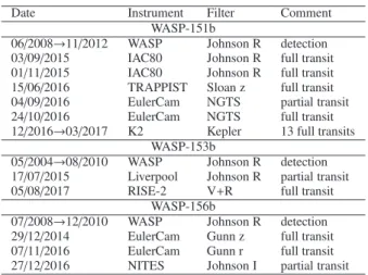
Lithium is detected in WASP-151 and WASP-153, with an equivalent width of 17 mÅ and 98 mÅ, corresponding to an abundance log A(Li) of 1.73 ± 0.05 and 2.77 ± 0.05 respectively. This implies an age of several Gyr and several Myr respectively. There is no significant detection of lithium in WASP-156, with an equivalent width upper limit of 11 mÅ, corresponding to an abundance upper limit of log A(Li) < 0.2. This implies an age of at least 500 Myr (Sestito & Randlich 2005).
The rotation rate (P = 14.8±4 d) implied by the v sin i∗gives a gyrochronological age of ∼ 1.80+2.03
−1.00 Gyr using theBarnes (2007) relation for WASP-151. Similarly, the rotation rate of P = 11.7 ± 2 d gives an age of ∼ 1.21+1.19
−0.60Gyr for WASP-153, and the rotation rate of P = 12.6 ± 4 d gives an age of ∼ 0.58+0.51 −0.31 Gyr for WASP-156.
Finally from Teff, log g and [Fe/H], we inferred stellar mass and radius estimates using theTorres et al. (2010) calibration. The parameters and error bars obtained from this analysis are listed in the section stellar parameters of Table3.
3.2. System Parameters 3.2.1. Transit and RV analysis
We followed the same method to perform the parameters’ in-ference for the three systems. We analysed jointly all the ra-dial velocity and photometric datasets available for a given sys-tem. To model the radial velocity and photometric data, we used the Python packages ajplanet11 (Espinoza et al. 2016) and batman11(Kreidberg 2015) respectively. In order to decrease the correlation between the parameters of our model and ease the fit, we adopted the parametrisation suggested byEastman et al.
(2013) with Rp/R∗the ratio of the planet’s radius to that of the star, P the orbital period, tcthe planet’s time of inferior conjunc-tion, √e cos ω∗and √e sin ω∗where e is the orbital eccentricity and ω∗is the stellar orbital argument of periastron, K the radial velocity semi-amplitude, i the orbital inclination, a/R∗ the ra-tio of the planet’s orbital semi-major axis over the stellar radius, v0 the systemic radial velocity, u and v the two coefficients of the limb-darkening quadratic law. To this set of parameters we added a logarithmic multiplicative jitter factor (ln fσ) for each instrument to account for a possible bias in the data’s error bars 11 Several of the Python packages used for this work are publicly
avail-able on Github: ajplanet at https://github.com/andres-jordan/ajplanet, batman at https://github.com/lkreidberg/batman, emcee at https://github.com/dfm/emcee, ldtk at https://github.com/hpparvi/ldtk
due to overestimated, underestimated or even non-considered sources of noise (see Baluev 2009). Finally, we added a pa-rameter for the shift of the radial velocity zero point between two instruments (∆RV) and three coefficients to model a linear or quadratic variation of the out-of-transit relative flux (∆Foot, ∆F′ootand ∆F
′′
oot) when it was necessary. The final list of main parameters is Rp/R∗, P, tc, √e cos ω∗, √e sin ω∗, K, cos i, a/R∗, v0, u and v, ln fσ, ∆RV, ∆Foot, ∆F′ootand ∆F
′′ oot.
To infer accurate values for these parameters, we used the maximum a posteriori (map) estimator of the Bayesian inference framework (e.g.Gregory 2005). The prior probability density functions (pdf) assumed for the parameters are given by Table A.4. Along with the posterior pdf provided in Table3, it allows for a qualitative assessment of the impact of the prior on the inferred values.
The prior on the limb darkening coefficients deserves a specific consideration. We used Gaussian pdfs whose first two moments were defined using the Python package ldtk11 (Parviainen & Aigrain 2015). Using a library of synthetic stellar spectra, it computes the limb darkening profile of a star, observed in a given spectral bandpass (specified by its transmission curve), and defined by its Teff, log g and [Fe/H]. Provided the values and error bars for these stellar parameters and the spectral band-pass, ldtk uses a Markov Chain Monte Carlo (mcmc) algorithm to infer the mean and standard deviation of the Gaussian pdfs for the coefficients of a given limb-darkening law (quadratic in our case). ldtk relies on the library of synthetic stellar spec-tra generated by Husser et al. (2013). It covers a wavelength range, from 500 Å to 5.5 μm , and a stellar parameter space de-limited by: 2 300 K ≤ Teff ≤ 12 000 K, 0.0 ≤ log g ≤ +6.0, −4.0 ≤ [Fe/H] ≤ +1.0, and −0.2 ≤ [α/Fe] ≤ +1.2. This pa-rameter space is well within the requirements of this study (see Tables1and3)
The likelihood functions used are multi-dimensional Gaus-sians, including logarithmic multiplicative jitter factors as de-scribed by Baluev (2009). To estimate the map and infer re-liable error bars, we explored the parameter space using an affine-invariant ensemble sampler for mcmc thanks to the Python package emcee11 (seeForeman-Mackey et al. 2013;Hou et al.
2012). We adapted the number of walkers to the number of free parameters in our model. As a compromise between the speed and the efficiency of the exploration, we chose to use ⌈nfree× 2.5 × 2⌉/2 walkers, where nfreeis the number of free parameters and ⌈ ⌉ the ceiling function. This allows to have an even number of walkers which is at least 2 times (∼ 2.5 times) the number of free parameters, as suggested byForeman-Mackey et al. (2013). The introduction in the model of a multiplicative jitter fac-tor complicated the exploration of the parameter space since it introduced local maxima. For the affine-invariant ensemble sampler mcmc algorithm implemented by emcee, when differ-ent chains converge towards differdiffer-ent disconnected maxima, the exploration becomes less efficient (the acceptance fraction of the chain decreases). Consequently, we separated the exploration into two phases. In a first exploration, we used values randomly generated from the priors as initial values for the free parame-ters. This first exploration allowed us to locate several (usually two) local maxima, to extract the global maximum (the one with the highest posterior probability) and to estimate its location and 68 % confidence level interval. Then we ran a second exploration to precisely sample the global maximum. For this one, the ini-tial values were randomly generated with normal distributions whose mean and standard deviation were set accordingly to the location and width of the global maximum found by the previous step. The final best-fit values for each parameter were estimated
from this second exploration after removing any residual burn-in phase with the Geweke algorithm (seeGeweke et al. 1992). The mapvalue for each parameter was finally estimated with the 50th percentile of the associated marginal posterior distribution. The extrema of the 68 % confidence level intervals were estimated with the 16th and 84th percentiles. These values are reported in Table3.
In Table3, we also reported the map and the 68 % confidence level interval for the secondary parameters. As opposed to the main (or jumping) parameters described in the first paragraph of this section, secondary parameters are not used in the parametri-sation chosen for our modeling and are not necessary to perform the mcmc exploration. However, they provide quantities that can be computed from main parameter’s values and are of interest to describe the system. The secondary parameters that we com-puted were: ∆F/F the transit depth, i the orbital inclination, e the eccentricity, ω the argument of periastron, b the impact parame-ter, D14 the outer transit duration (duration between the 1stand 4thcontact), D23 the inner transit duration (duration between the 2nd and 3rdcontact), R
p the planetary radius, Mp the planetary mass, a the semi-major axis, τcircthe timescale for the circular-isation of the orbit, Fithe incident flux on the top of the plan-etary atmosphere, Teqthe equilibrium temperature of the planet (assuming an albedo of 0), H the scale height of the atmosphere assuming a mean molecular weight of 2.2 g/mol, ρ∗ the stellar mean density and log g the stellar log gravity. Both ρ∗and log g are, in this case inferred from the transit profile12. These
esti-mates are marked with (tr.) in Table3. After the full mcmc anal-ysis, we computed the value of all these secondary parameters from the main parameters values and at each step of each walker of the second emcee exploration. Then we estimated their map and 68 % confidence level interval with the same method than the main parameters.
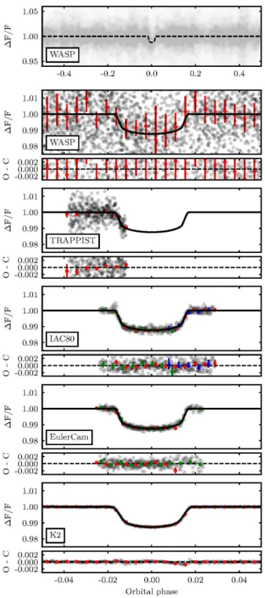
The specificities for the analysis of each system were: WASP-151: The exposure times of the WASP, IAC80, Euler-Cam and TRAPPIST data are all below 90 s which is negligible compared to the time scale of the transit variations (typically 30 min for the transit ingress and egress). However the exposure time of the K2 light-curve is 29.424 min. Consequently, for the model of the K2 data, we supersampled13the model by a factor
10. This means that for each exposure, we computed the instan-taneous value predicted by the model at 10 different times evenly distributed over the exposure and then used the average of these 10 values as the model value for the whole exposure.
A first analysis of this system showed a linear trend in the residuals of the TRAPPIST and the September IAC80 light curves. We also noticed a more complex behavior in the Novem-ber IAC80 light curves that we decomposed into two linear trends with a break point at t = 2 457 328.5022 HJD. There-fore we split the November IAC80 light curves into two and added 8 parameters to our model to account for these lin-ear variations of the out-of-transit (2 per light-curve). When doing so, we used the time of the first sample (tmin) as the origin for the linear function: ∆Foot +(t − tmin) ∆F′oot). tmin is equal to 2 457 187.753440000124, 2 457 269.443920060061, 2 457 328.353823559824, 2 457 328.502696809825 HJD for the TRAPPIST, the September IAC80, the first part and the second part of the November IAC80 light-curves respectively.
12 To obtain log g, we also used the estimate of the stellar mass obtained
in the next section (3.2.2).
13 We refer the reader toKipping(2010) for more details regarding the
We re-analyzed jointly all the datasets with these 8 addi-tional free parameters in our model. The inferred parameter val-ues and error bars are reported in Table3. Figure2and3show the photometric and radial velocity data phase folded at the best-fit ephemeris (see Table3) with the best-fit model and residuals. The error bars displayed take into account the best-fit jitter val-ues obtained by the Bayesian inference (see Table3).
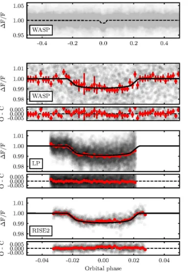
WASP-153: The exposure times of the WASP, Liverpool and RISE-2 data being below 40 s, no supersampling was required for this system. The analysis didn’t show any abnormal behav-ior. The inferred parameter values and error bars are reported in Table 3 and the Figures4 and5 show the photometric and radial velocity data phase folded at the best-fit ephemeris (see Table 3) with the best-fit model and residuals. The error bars displayed take into account the best-fit jitter values obtained by the Bayesian inference (see Table3).
WASP-156: The exposure times of the WASP and NITES data being both below 40 s, no supersampling has been applied for those two datasets. The exposure time of the EulerCam data be-ing around 80 s and the be-ingress and egress for this system bebe-ing relatively short (∼ 10 min), we decided to supersample the model by a factor 4.
A first analysis of this system showed that the 2 datasets collected with EulerCam were not compatible. The 2014 Euler-Cam dataset displayed a very pronounced V-shape that was not supported by the other datasets. As described in Section2.2.1, this dataset was identified earlier as affected by large PSF varia-tions, and stellar counts in the non-linear regime of the EulerCam CCD. So we decided to discard it from the final analysis. We also noticed that the residuals of the 2016 EulerCam light-curve seemed to exhibit a quadratic trend and introduced 3 additional parameters to our model to account for a possible quadratic vari-ation of the out-of-transit level. When doing so, we used the time of the first sample (tmin = 2 457 700.517166 HJD) as the ori-gin for the quadratic function: ∆Foot+(t − tmin) ∆Foot′ +(t − tmin)2∆F′′′oot).
We re-analyzed jointly all the datasets with these 3 addi-tional free parameters in our model. The inferred parameter val-ues and error bars are reported in Table3. Figure6and7show the photometric and radial velocity data phase folded at the best-fit ephemeris (see Table3) with the best-fit model and residuals. The error bars displayed take into account the best-fit jitter val-ues obtained by the Bayesian inference (see Table3).
3.2.2. Stellar modelling
In Section 3.1, we derived stellar masses and radii from Teff, log g and [Fe/H] using the Torres et al. (2010) calibration and ages using lithium abundances and gyrochronology. If those two age estimates seem to agree for our three systems, the Lithium constraint on the age is very weak and gyrochronol-ogy is known to sometimes contradict other ages estimators like isochronal ages (e.g.Buzasi et al. 2016;Angus et al. 2015;
Kovács 2015;Maxted et al. 2015b). Furthermore, the additional constraint brought by the stellar density inferred from the transit and a dedicated modelling of the star should result in more ac-curate estimates of the stellar masses and radii. Consequently to provide a more comprehensive view of our three systems,
we modelled the stars using the Fortran software bagemass14
(Maxted et al. 2015a).
Bagemassrelies on a grid of stellar models15produced with the garstec stellar evolution code (Weiss & Schlattl 2008). This grid covers the mass range between 0.6 to 2.0 M⊙, the initial metallicity range between −0.75 to 0.55 dex and the age range between the end of the pre-main-sequence phase up to 17.5 Gyr (or a maximum radius of 3 R⊙depending on which one occurs first). In order to obtain stellar properties for any mass, metal-licity and age within these ranges, and not only for the points in the grid, bagemass uses the cubic spline interpolation algorithm pspline16. Given measurements (values and error bars) for the Teff, [Fe/H] and density (ρ∗) of the star studied, it then explores this parameter space using a mcmc method which computes the posteriorprobability as a function of mass and age.
Using the Teffand [Fe/H] estimates provided by the spectral analysis and the stellar density estimates obtained from the anal-ysis of the transit (see Section3.2and Table3), we obtained es-timates and 68 % confidence interval error bars for the ischronal age and the mass of our three stars17. These values are reported
in Table 3. Fig 8 shows the marginalized probability distribu-tion in the Hertzsprung–Russell diagram along with the best-fit evolutionary model and isochrones for our three stars. To pro-vide more robust error bars, the error bar propro-vided in Table3 for the mass estimate (M∗(tr. + ev. track)) is the square-root of the quadratic sum of the internal error and the sensitivities to the mixing length parameter and the Helium-enhancement. Finally, we also computed new estimates for the secondary parameters of the transit and RV analysis (see Section3.2.1) which rely on the stellar mass and radius estimates. The most sensitive of those pa-rameters are Rp, Mp, ρp, H and Fi. We reported these estimates in Table3.
The interpretation of the isochronal age estimate is the subject of Section 4.3, so we will now focus on the stellar mass and radius estimates. For WASP-151, this analysis pro-vides estimates that are compatible within one sigma with the ones obtained with the Torres et al. (2010) calibration (Sec-tion3.1). However for WASP-153 and WASP-156, it’s not the case. The stellar modelling predicts a significantly bigger radius for WASP-153 and a significantly lower radius for WASP-156 while the masses are compatible within one sigma (see Table3). This difference is mainly explained by the difference in log g be-tween the spectroscopic and transit analyses (see tr. and spec. values of log g in Table3). The comparison of log g estimates from spectroscopy made bySmalley(2005) showed that a real-istic error bars for a log g estimator from spectroscopy is ∼ 20 %, while the one inferred from the transit density is more direct and more robust with typical uncertainties . 5% depending on the quality of the light-curve and the photometric stellar variability. As described in Section2.1, our three stars are not particularly active. We will thus rely on the stellar mass and radius estimates obtained in this section for the rest of the paper, even if we show
14 We used the version 1.1 available at
http://sourceforge.net/projects/bagemass.
15 bagemassprovides several grid with different mixing length (α MLT
equal 1.78 or 1.50) and different Helium-enhancement (0.0 or 0.2). For this work, we used the default values which correspond to no Helium-enhancement and αMLT=1.78. However, in TableA.5, we present
esti-mates of the sensitivity of the results to this assumptions.
16 The pspline algorithm is available at
http://w3.pppl.gov/ntcc/PSPLINE
17 The complete output table provided by bagemass is available in
in Fig 9,10 and Table3 the estimates relying on the spectro-scopic log g for completeness.
4. Discussion and conclusion
Table 3 give us an exhaustive picture of these 3 systems and allows us to put them in context.
WASP-151b and WASP-153b are relatively similar. Their masses of 0.31 and 0.39 MJupand semi-major axes of 0.056 AU and 0.048 AU respectively indicate two Saturn-size objects around early G type stars of V magnitude ∼ 12.8. WASP-156b’s radius of 0.51 RJupsuggests a Super-Neptune18and makes it the smallest planet ever detected by WASP. Its mass of 0.128 MJup is also the 3rd lightest detected by WASP after WASP-139b
(Hellier et al. 2017) and WASP-107b (Anderson et al. 2017).
Also interesting is the fact that WASP-156 is a bright (magV = 11.6) K type star.
In the following two sections, we compared the posi-tion of our three planets in the mass-radius diagram with the isochrones of Baraffe et al. (2008) to constrain their composi-tion.Baraffe et al.(2008) provide two types of models, one with-out irradiation and one with the irradiation received at 0.045 AU from the Sun. Given the semi-major axes of our planets, the lat-ter is the most suited to this study and is the one we used in Fig9. We refer readers interested in the details of these models to the associated publication.
In the third section, we discuss the age estimates of those three systems. More specifically, we address the apparent dis-crepancy between the gyrochronological and isochronal ages and the possible insight that it provides regarding the migration mechanism of the planets in these systems. Finally, the fourth section is devoted to the impact of these three planets on our understanding of the Neptunian desert (Mazeh et al. 2016). 4.1. Two hot Saturns: WASP-151b and WASP-153b
WASP-151b and WASP-153b’s position in the mass-radius di-agram indicate two low density gaseous planets (see Fig 9). Their masses are close to the one of Saturn but their radii are significantly bigger, especially for WASP-153b. Relying on its isochronal age and its relative position compared to the isochrones ofBaraffe et al.(2008), WASP-151b should have a heavy-element mass fraction slightly smaller than 2 %. Simi-larly, WASP-153b’s heavy-element mass fraction should be sig-nificantly smaller than 2 %. Knowing that WASP-151 has a metallicity compatible with the one of the Sun, that WASP-153 is super-metallic ([Fe/H] = 0.34 ± 0.11 dex) and that the Sun’s heavy element mass fraction is close to 2 % (e.g.Baraffe et al. 2008), these heavy element mass fractions inferior to 2 % are unlikely. Consequently, WASP-151b appears to be slightly more bloated than the models predict and WASP-153b exhibits a sig-nificant radius anomaly. This interpretation is, of course, depen-dant on the accuracy of our mass, radius and age estimates. As shown in Fig9, if we rely on the planetary radius inferred from the purely spectroscopic stellar parameters (Section3.1), WASP-151b and WASP-153b are compatible within one sigma with the model ofBaraffe et al.(2008). However as discussed in Sec-tion3.2.2, these estimates appear less precise and less accurate than the ones above, which rely on the stellar density inferred from the transit and stellar models.
18 Bakos et al.(2015) defined the class of Super-Neptunes as the
plan-ets whose mass lies between 0.054 MJup (the mass of Neptune) and
0.18 MJup(halfway between the mass of Neptune and Saturn).
Given the relatively high incident flux received by these two planets (460 Fi,⊕for WASP-151b and 1400 Fi,⊕ for WASP-153b), the radius anomalies that they exhibit was expected. Indeed, it is in agreement with the empirical thresholds de-fined byMiller & Fortney(2011) andLopez & Fortney(2016) for an abnormally inflated radius: R > 1.2 RJup and Fi > 2 108 erg.s−1.cm−2 ∼ 150 F
i,⊕. WASP-153b exceeds signifi-cantly both thresholds and WASP-151b exceeds the incident flux threshold, but is slightly below the radius threshold.
4.2. A warm Super-Neptune: WASP-156b
WASP-156b’s position in the mass-radius diagram suggests a composition significantly different from the ones of WASP-151b and WASP-153b. Baraffe et al.(2008) models indicate a high heavy element mass fraction around 90 %, in agreement with the one of Neptune and Uranus (Helled & Guillot 2017), de-picting WASP-156b as a warm Super-Neptune. Super-Neptunes with precise determination of the mass and radius (better than 15 %) are relatively rare since only 9 of these objects are known at the moment: Kepler-9c (Torres et al. 2011), Kepler-35b (Welsh et al. 2012), Kepler-101b (Bonomo et al. 2014), HATS-7b (Bakos et al. 2015), HATS-8b (Bayliss et al. 2015), WASP-107b (Anderson et al. 2017), WASP-127b (Lam et al. 2017), WASP-139b (Hellier et al. 2017) and WASP-156b. Amongst this class of planets, WASP-156b, as a warm (Teq = 970 K) and dense (ρp = 1.0 ρJup) Super-Neptune, is particularly interest-ing to investigate the gaseous to ice giant transition as described byAnderson et al.(2017) andBakos et al.(2015). WASP-156 is also currently the brightest Super-Neptune host star, with a V magnitude of 11.6, making it a target of prime interest for future atmospheric characterisation.
4.3. Discrepancy between the ages estimators, an insight on migration mechanisms ?
In Sections 3.1and3.2.2, we derived ages for our three stars with Lithium abundance, gyrochronology and isochrone fitting. These results are reported in Table4. The tendency that arises from this table is that our stars tend to have isochronological ages that are significantly higher than their gyrochronological ages. This tendency, limited here to three cases, has already been observed byMaxted et al. (2015b) for a broader sample of 28 transiting exoplanets where at least half of the sample exhibits this discrepancy. Interestingly for more than 80 % of the stars in this sample, and for our three stars, the planetary companion is a short period (< 5 days) giant planet.
Discrepancies between gyrochronological and isochrono-logical ages have been reported by several studies and not only in the context of planet host stars, see for exam-ple Angus et al. (2015); Kovács (2015); Buzasi et al. (2016).
Maxted et al. (2015b) found that gyrochronological age
esti-mates were significantly lower than the isochronological ones for about half of their sample of planetary hosts.Kovács(2015) reached a similar conclusion from a galactic field stars sam-ple. FinallyBuzasi et al.(2016) andAngus et al.(2015) brought to light inconsistencies in the gyrochronological age estimator when applied to different samples. This problem is thus complex and has multiple facets. Consequently, it will not be solved solely by the 3 stars discussed in this paper. However they can give us insights regarding the specific question of the underestimation provided by the gyrochronological age estimator observed for a fraction of the short period planet host stars population.
To explain the hot giant planet population, the core-accretion scenario requires a mechanism to migrate these planets from their formation location, beyond the ice line, to the vicinity of their parent star. There is currently two mechanisms debated in the literature for this migration: disk driven migration (e.g.
Lin et al. 1996;Ward 1997) and high eccentricity migration (e.g.
Rasio & Ford 1996;Fabrycky & Tremaine 2007). The main ob-servational arguments to favour one over the other are: Spin-Orbit misalignment (e.g. Naoz et al. 2012), stellar metallicity (e.g.Dawson & Murray-Clay 2013), the presence of additional companions (e.g.Schlaufman & Winn 2016) and the Roche sep-aration (e.g.Nelson et al. 2017).
Under the light of Table 4 and the study performed by
Maxted et al.(2015b), we suggest that a gyrochronological age significantly smaller than the isochronal one could be an evi-dence to identify the mechanism responsible for the migration of giant planets. A gyrochronological ages significantly lower than the isochronological one might indeed be explained by the important transfer of angular momentum from the giant planet to the star during the tidal circularisation of the planet’s orbit involved in high eccentricity migration. On the contrary, disk driven migration implies an exchange of angular momentum be-tween the planet and the disk and cannot directly explain an increase of the stellar rotation. Furthermore, contrary to disk driven migration, high eccentricity migration is not bounded to the short protoplanetary disk lifetime and can occur at an older stage of the system amplifying even more the discrep-ancy between the two age estimates. If this hypothesis is con-firmed for stars hosting short period planets, a gyrochronological age significantly smaller the isochronal age (e.g. the three host star presented in this paper) would indicate that the planet mi-grated through high-eccentricity migration while a gyrochrono-logical age compatible with the isochronal one (e.g. WASP-33
Collier Cameron et al. 2010) would suggest a disk driven migra-tion (or an in-situ formamigra-tion).
Obviously, a more thorough analysis is necessary to investi-gate all the possible implications behind this hypothesis. Such an analysis is out of the scope of this paper but we think that this hy-pothesis is worth investigating. In this context, a search for long period companions that might have triggered the high eccentric-ity migration or an independent age estimate through asterosis-mology with TESS (Campante et al. 2016) or Plato (Rauer et al. 2014) would be particularly interesting.
Table 4.Age estimates of WASP-151, WASP-153 and WASP-156. Iso. stands for isochronal age, Gyro. for gyrochronological age and Li for the age constraint based and Lithium abundance.
Star Iso. [Gyr] Gyro. [Gyr] Li
WASP-151 5.13+1.33 −1.33 1.80 +2.03 −1.00 several Gyr WASP-153 4.00+0.77 −0.77 1.21 +1.19 −0.60 several Myr WASP-156 6.50+4.03 −4.03 0.58+0.51−0.31 &500 Myr
Note: The isochronal age estimates in this table are obtained us-ing the mean value of the marginalized posterior distribution of the age. For WASP-151 and WASP-153, these are compati-ble with the maximum-likelihood estimate. However for WASP-156, it is not the case since the latter give an age of 0.5 Gyr (see TableA.5).
4.4. Three planets at the border of the Neptunian desert As described in the introduction,Mazeh et al.(2016) studied the distribution of the planet population in the orbital period, mass and radius domain and reported the lower and upper mass and radius boundaries of the short period Neptunian desert. Fig10 shows that WASP-151b and WASP-153b lie near the upper boundaries of the desert, while WASP-156b stands well inside it. The authors mentioned that the period limit of the desert was not well constrained, however they also indicated that these bor-ders delineate the boundaries for periods below 5 days, which is the case of WASP-156b. Understanding the differences be-tween 156b on one side and 151b and WASP-153b on the other side might allow to shed light on the mecha-nism responsible for the upper boundary of the Neptunian desert.
Mazeh et al.(2016) proposed two explanations for the origin of the upper boundary of the desert:
– Gaseous planets can’t exist below the upper boundary, be-cause they would lose their gaseous envelope due to stellar insolation (e.g.Lopez & Fortney 2014) or Roche-lobe over-flow (e.g.Kurokawa & Nakamoto 2014).
– Gaseous planets are formed further away from their parent star and can’t migrate below the upper boundary, because at this distance from the star the disk is not dense enough to sustain inward migration.
While a detailed analysis of the origin of the Neptunian desert is beyond the scope of this paper, it is still interesting to look into the similarities and differences between 156b and WASP-151b/WASP-153b since they might provide useful hints on the nature of this desert. These three planets possess similar orbital parameters (see Table3). Their ages are subject to caution (as discussed in Section4.3), but a given estimator provides similar ages for these three stars. Their gyrochronological ages indicate relatively young systems (∼ 1 Gyr for 151 and WASP-153 and ∼ 0.5 Gyr for WASP-156), while their isochronal ages indicate ∼ 5 Gyr old systems. However, their radiative envi-ronments are significantly different. 151b and WASP-153b receive a higher bolometric irradiation (460, 1400 and 150 Fi,⊕for WASP-151b, WASP153b and WASP-156b respec-tively). Moreover the spectral type of their host stars are different (early G for 151 and 153 and early K for WASP-156) implying a different spectral content of the irradiation, es-pecially in extreme ultra-violet (EUV). The EUV flux is partic-ularly interesting in this context since it is the main contribu-tor for exoplanet atmosphere evaporation.Lecavelier Des Etangs
(e.g. 2007) provided estimates for the EUV flux emitted by stars of different spectral types. According to these estimates, the EUV flux received by WASP-156b is ∼ 3 times higher than the one received by WASP-151b and WASP-153b, FEUV@1AU is 15 erg.cm−2.s−1 for K type stars and 5 erg.cm−2.s−1 for G type stars. This suggests that photo-evaporation is the mechanism responsible for the presence of WASP-156b below the upper boundary of the short-period Neptunian desert. WASP-156 may be in the process of losing its gaseous envelope in a short-lived evolutionary phase which places it within the underpopulated short-period Neptunian desert.
Finally, in the context of the hypothesis formulated in Sec-tion4.3, it is also interesting to mention the alternative expla-nation defended byMatsakos & Königl(2016) for the origin of the Neptunian desert. The authors present the desert as the re-sult of high-eccentricity migration of planets that arrive in the vicinity of the Roche limit of their host star and suggest that the