Tracking Illiquidities in Intradaily and Daily Characteristics

Tracking Illiquidities in Intradaily and Daily

Characteristics

Serge Darolles

Gaëlle Le Fol

Gulten Mero

January 14, 2011

Abstract

In this article, we distinguish between two types of liquidity problems called re-spectively liquidity frictions and illiquidity events. The first one is related to order imbalances that are resorbed within the trading day. It can be assimilated to "imme-diacy cost" and impacts the traded volume at the intraday and daily frequencies while affecting the price increments only at the intraday periodicity. The second one is inher-ent to the long lasting liquidity problems and is responsible for the time-dependence of the daily returns. We extend the MDHL framework of Darolles et al. (2010) to account for the presence of the illiquidity events. We then propose a two-step signal extraction formulation of the MDHL model in order to separate the two liquidity problem impacts on the daily returns and volume. We also provide, for a set of FTSE100 individual stocks, long lasting illiquidity indicators.

JEL classification: C51, C52, G12

Key words: Volatility-volume relationship, mixture of distribution hypothesis, liq-uidity shocks, information-based trading, liqliq-uidity arbitrage, Markov regime switching stochastic volatility model.

∗_{LYXOR AM and CREST-INSEE, France, serge.darolles@ensae.fr, 15 Bd Gabriel Péri (Timbre J320)}

92245 Malakoff cedex

†_{University of Paris-Dauphine, DRM Finance (CEREG) and CREST-INSEE, France,}

gaelle.le-fol@ensae.fr, 15 Bd Gabriel Péri (Timbre J320) 92245 Malakoff cedex

‡_{University of Rennes 1, CREST-INSEE and CREM-CNRS, France, gulten.mero@ensae.fr, 15 Bd Gabriel}

Péri (Timbre J320) 92245 Malakoff cedex, Tel. +33 (0)6 30 01 33 70.

1

Introduction

Recent financial crisis, such as that of August 2007, highlight the importance of liquidity in the viability of financial markets. Liquidity problems can be inherent to both transaction costs and to the risk that immediacy may completely dry up. On the one hand, liquidity problems can be assimilated to the "cost of immediacy" supported by liquidity demanders. At the same time, they represent a source of trading for liquidity suppliers, such as intraday statistical arbitragers, who exploit short term negative correlatin and provide immediacy when needed. In return, they require a liquidity premium for bearing the inventory risk as well as the risk of exchanging against an informed trader. On the other hand, liquidity problems represent an important source of risk to any investors. This risk is related to the possibility that liquidity might disappear from the market resulting in important losses. To illustrate this point, recall that during the week of August 6, 2007, a number of high-profile and highly successful quantitative long/short equity hedge funds experienced unprecedented losses. As discussed by Khandani and Lo (2007), "the losses were initiated by the rapid unwinding of one or more sizable quantitative equity market-neutral portfolios [which] was likely the result of a sudden liquidation by a multi-strategy fund or proprietary-trading desk, possibly due to margin calls or a risk reduction". Brunnermeier and Pedersen (2009) explain how these [ destabilizing] margins resulting from imperfectly informed financiers amplify with trader capital losses as well as highly volatile markets and cause liquidity dry up spirals. This can be a source of trading for another type of statistical arbitragers who exploit positive long term correlations.

Measuring liquidity is not an easy task since account should be taken not only of the distinction between the two aforementioned liquidity problems, but also of their dynamic character through time. This study exploits the framework of Darolles et al. (2010) in order to analyze liquidity risk affecting stock markets and extract a dynamic liquidity measure from the observed time series of daily returns and traded volume.

Based on Grossman and Miller (1988) framework, Darolles et al. (2010) suggest that the 2

presence of liquidity frictions due to trade asynchronization motivates the intervention of liquidity arbitragers which increases the daily traded volume. The liquidity arbitragers, who track market imperfections, provide liquidity when needed. They react to market volatility rather than being responsible for it and contribute to the resorption of (part of) the intraday volatility resulting from liquidity shocks. Assuming that the liquidity frictions are resorbed within the trading day, the authors extend the standard mixture of distribution hypothesis (MDH in the following) model of Tauchen and Pitts (1983) by accounting for liquidity shock impact on stock returns and traded volume. The resulting MDHL1

model explains the contemporaneous stochastic dependence between daily volatility and volume by the interaction of information arrivals and liquidity frictions. It is a structural model allowing to decompose the daily traded volume into two components due to two unobservable variables, namely, information and liquidity shocks. The MDHL model provides a static stock-specific liquidity indicator using daily data. The liquidity events are a source of trade rather than a source of risk for the liquidity arbitragers2

. For the active traders, the liquidity frictions result in transaction costs only3

.

The MDHL model does not account for long lasting liquidity problems. However, as-suming that the liquidity events are resorbed within the trading day is quite unrealistic. In particular, liquidity problems can last several days and even exacerbate. In this case, the closing prices will not reveal the full information set. These situations, which convey the signal that the market faces difficulties to maintain liquidity, can be transformed in liquidity dry up premises in the sense of Brunnermeier and Pedersen (2009). As discussed by the authors, market liquidity can suddenly and radically dry up when market participants face destabilizing funding constraints. The margins are called destabilizing when they increase with market price volatility and arise when imperfectly informed financiers4

interpret price

1

Mixture of distribution hypothesis with liquidity shocks.

2

They are supposed to liquidate their positions at the next intraday date once prices are back to equilib-rium as new active traders arrive with the opposite order imbalance.

3

They exchange at an disadvantageous price at the profit of the arbitrage participants unless they decide to report their trade to the next (intraday) exchange.

4

In the Brunnermeier and Pedersen (2009) framework the "financiers" represent a group of market

variance due to liquidity frictions as fundamental volatility. The extreme case is related to market dry up liquidity persisting over several days which leads to liquidity spirals and liquidity crisis. The MDHL model provides a time-invariant stock-specific liquidity measure in normal time periods when the market is not under stress. However, as liquidity is time-varying and persistent [see for example Amihud (2002), Chordia et al. (2001b), Chordia et al. (2001a), Hasbrouck and Seppi (2001), Huberman and Halka (1999) and Jones (2001)], an interesting extension would be to construct a dynamic liquidity measure.

In this paper, we extend the MDHL model in order to account for long lasting liquidity problems and thus provide a structural interpretation of the dynamic properties of daily returns and volumes. The idea behind our reasoning is to distinguish between two types of liquidity problems that we call liquidity frictions and illiquidity events, respectively. On the one hand, the liquidity frictions are short lasting and are represented by the intraday order imbalances that are resorbed within the trading day. They impact the traded volume at the intraday and daily frequencies while affecting the price volatility only at the intraday periodicity. The liquidity frictions are a source of trade for the liquidity arbitragers who liquidate their positions once prices are back to the equilibrium in order to cash the liquidity premium. They can also be assimilated to the cost of immediacy supported by the active traders. The liquidity frictions correspond to the latent variable Lt of the MDHL model.

On the other hand, the illiquidity events correspond to situations where information hitting the market is not entirely incorporated into prices on its arrival day if liquidity problems are long lasting. In fact, the market is said to be affected by illiquidity events when only part of market participants are able to trade for any reason. This is due for example to limited trading capacity of traders in the sense of Brunnermeier and Pedersen (2009) which are due to important margin calls or limited exogenous wealth. In this case, their reservation prices reflect only part of the incoming information. These situations are inherent to liquidity risk supported by the market participants who can not liquidate their positions at the fully re-ticipants who finance speculators’ positions. The latter group of traders can be assimilated to the liquidity arbitragers of our world.

vealing information price. However, they can be a source of trading for statistical arbitragers who exploit long term dynamics of the time series of returns.

Second, we exploit the triangular structure of the MDHL model to build a two-step methodology in order to extract dynamic liquidity latent factors using daily time series of returns and volume. To do so, we first use a Markov regime switching stochastic volatility model to extract the effect of information shocks from the daily price change time series. In our framework, the dynamics of the information flow variable is due to the presence of illiquidity events. Then, conditional on the estimated variables of the first step, a simple Kalman filter allows us to extract the latent liquidity factor using daily volume observations. This procedure enables us to: (i) capture the impact of illiquidity events in the daily price change and volatility dynamics; (ii) separate the impact of both, the occurrence of illiquidity events and the persistence of liquidity frictions, on the serial correlation of the daily traded volume.

Finally, the contribution of this paper is threefold:

(i) The extended MDHL model accounts for the most harmful side of liquidity problems, the long lasting ones, which make prices deviate from the fundamental value of the assets for a long time.

(ii) Our econometrical set up enables us to isolate the effects of both types of liquidity prob-lems on stock returns. The liquidity frictions, due to trade asynchronization and resorbed within the trading day, increase the daily traded volume. Their impact is measured by the average-volume parameter related to the latent variable Lt, which corresponds to the static

liquidity measure developed in Darolles et al. (2010). This liquidity indicator is useful in practice since it allows market participants, such as statistic arbitragers, to detect, on aver-age during a given period of time, the presence of liquidity frictions at the individual stock level and thus select the candidates with significant liquidity-based traded volume. On the other hand, the presence of "illiquidity events" exceeding the intraday perspective, is cap-tured from the dynamic properties of daily price changes. This provides additional insights

on stock liquidity and enables market participants to identify equities affected by liquidity risk.

(iii) From a theoretical point of view, our extended framework provides a structural interpre-tation of the dynamic properties of return time series. The short term liquidity frictions are responsible for intraday dynamics of return and volatility, while the long lasting illiquidity frictions result in daily positive serial correlation of stock returns and squared returns. When working with daily data, the intraday effect of the liquidity frictions can be inferred from the trading volume. From a practical point of view, distinguishing between the two liquidity problems has direct implications for statistical arbitrage strategies. Actually, the statistical arbitrage traders compute the sample serial correlation of stock returns and pick up positive serially correlated stocks to build up momentum strategies, while using the negative serially correlated ones to construct mean reverting strategies. Based on the extended MDHL frame-work, we suggest that the sample serial correlation coefficients are not sufficient criteria to select stocks for statistical arbitrage strategies. In particular, the empirical autocorrelation functions are not efficient when the observed variables are heteroscedastic. We propose an alternative selection process directly derived from our theoretical framework. For example, a stock may have a first order serial correlation not significantly different from zero and still be affected by liquidity problems whose presence will be empirically detected using the parameters of our model.

The paper is organized as follows. Section 2 introduces our theoretical framework. We first summarize the MDHL model with information and liquidity shocks, and then provide an extended model accounting for long lasting liquidity problems. Section 3 presents our econometrical methodology to extract information and liquidity latent factors from the daily time series of returns and volume. In Section 4, we apply our econometrical set up to a group of individual stocks belonging to the FTSE100 and discuss the empirical results. Section 5 concludes the article.

2

Theoretical framework

In this section, we first provide a brief summary of the MDHL model with information and liquidity shocks developed in Darolles et al. (2010). Then, we relax the assumption that liquidity frictions are resorbed within the trading day and discuss the model implications. Finally, we propose a signal extraction formulation of the MDHL model in order to provide dynamic liquidity factors.

2.1

The MDHL model

We focus on a single-risky-asset market in which liquidity is determined by the demand and the supply of immediacy. We consider two types of market participants, J active traders and M liquidity arbitragers who trade in response to information flow and liquidity shocks, respectively. Each trading day t (t = 1, ..., T ) is considered as a succession of intraday market equilibria. The passage from the ith equilibrium to the next is triggered by information inflow It (i = 1, ..., It). New information modifies active trader expectations concerning the

liquidation value of the asset at the end of the trading day ˜P ; they decide to rebalance their positions in order to share risk through the market. It is assumed to be a random i.i.d.

variable. Let zij be the endowment shock of trader j (j = 1, ..., J) given the ith piece of

information. If all the active traders are present in the market, the aggregated endowment shock across traders is zero PJ_j=1zij = 0 and the ith equilibrium price Pi equals its fully

revealing information level.

However, within the ith equilibrium, the market may face a liquidity event due to asyn-chronization of order flows. The aggregated endowment shock of active traders being present in the market (J1 < J) represents the order imbalance: zi =

PJ1

j=1zij 6= 0. This generates

a 2-trading-date process in the sense of Grossman and Miller (1988) which extends from the ith to the (i + 1)th equilibria and comprises of 2 successive information arrivals hitting the market before trading at date 1 (ith equilibrium) and before trading at date 2 (i + 1)th

equilibrium, respectively. At date 1, liquidity arbitragers enter the market to provide imme-diacy by trading at an advantageous price at the expense of active traders. In this case, the ith transaction price differs from the fully revealing price. To cash the liquidity premium, arbitrage participants liquidate their positions at the (i + 1)th equilibrium (date 2 of the GM-process), as new active traders arrive with the opposite order imbalance. Because of the intervention of arbitrage traders, in the presence of liquidity shocks, the traded volume due to the ith piece of information is higher than it would have been if the market were perfectly liquid. The number of liquidity shocks affecting the market for a given trading day Lt is

considered to be random and conditionally independent of It.

Summing the within-day price changes and traded volume due to information and liq-uidity shocks, yields the daily price change ∆Pt and daily traded volume Vt. Assuming that

the liquidity frictions affecting the market at day t are resorbed before the end of the trading day, we show that conditional on It and Lt, ∆Pt and Vt are drawn from a bivariate normal

distribution: ∆Pt = σp p ItZ1t, (2.1) Vt = µatv It+ µlavLt+ σv p ItZ2t, (2.2) where σ2

p is the variance of intraday price change; µatv , σv2 are the mean and variance of

intraday traded volume due to information flow; µla

v is the mean of intraday traded volume

due to liquidity frictions5

; and Z1t, Z2t are mutually independent standard normal variables

(and independent of It and Lt). Equations (2.1)-(2.2) represent the MDHL model implying

that information flow impacts both daily price change and traded volume, while only daily volume is affected by random liquidity shocks.

We assume that, conditional on It, Lt has a binomial distribution: Lt ∼ B(It, p), with p

being the probability of occurrence of trade asynchronization. It follows that the expectation

5

The variance of intraday liquidity-based volume can be considered as o(JJ1) when added to σv2.

of the observed daily traded volume and its unconditional covariance with squared price change are respectively:

E(Vt) = µatv + pµ la v, (2.3) Cov(∆P_t2, Vt) = σ2p(µ at v + pµ la v )V ar(It). (2.4)

The MDHL model enables us to separate the daily traded volume − on average over a given test period − into two components due to information flow µat

v and liquidity shocks pµlav. In

particular, pµla

v represents a static liquidity measure determined by both the amplitude (on

average) of order imbalances µla

v and their probability of occurrence p. The model enables

us to detect the presence of intraday liquidity frictions by providing a stock-specific liquidity indicator using daily data.

2.2

The long lasting liquidity problems

Darolles et al. (2010) assume that the intraday liquidity shocks are resorbed within the trading day and do not impact the daily price change. In the MDHL model framework, this implies that: (i) the whole information hitting the market within a trading day is incorporated into the daily price change; (ii) the intraday liquidity frictions are resorbed within the trading day6

. However, liquidity problems may perpetuate through time and even exacerbate. The question is how to take account, in our framework, of the long lasting liquidity problems?

One natural generalization of our framework, is to simply allow for GM processes to extend across two successive trading days. To do so we should assume that a liquidity friction may occur at the last trade of the day. In this case, it would take more than a single day to prices to reach their fully revealing information level. Moreover, the dynamic properties of intraday price changes and traded volumes implied by Grossman and Miller (1988) and

6

In the MDHL model, there is no liquidity friction when the last trade of the day occurs

the standard MDHL frameworks would be verified for the daily time series. In particular, this extension would imply: (i) a negative serial correlation for the daily price changes; (ii) a positive serial correlation for the squared price increments and (iii) a negative serial correlation for the daily traded volume. The standard MDHL model would be a particular case of this extended framework when any liquidity friction occurs at the last exchange of the trading day. However, assuming that a single intraday liquidity friction (the last one) drives the dynamic properties of daily time series is quite unrealistic. In fact, the impact of a single intraday liquidity friction on daily price changes and volumes is negligible as compared to the cumulated impact of all of the intraday liquidity frictions and information arrivals hitting the market within a given trading day. In other words, even if the last liquidity friction is not resorbed within the trading day, its impact on the interdaily dynamics of the observed time series is blurred out when the number of pieces of information hitting the market is large. Thus, this extension seems not appropriate in accounting for the long lasting liquidity problems in frequently-traded stock markets.

Here, we consider another possible extension of the MDHL model in order to account for long lasting liquidity problems and thus provide a structural interpretation of the dynamic properties of daily returns and volumes. We distinguish between two types of liquidity problems that we call liquidity frictions and illiquidity events, respectively. The first one is related to short term liquidity problems represented by the intraday order imbalances which are resorbed within the trading day. They impact: (i) the traded volume at the intraday and daily frequencies and (ii) the price changes only at the intraday periodicity by inducing a negative serial correlation of intraday price inrements and positive serial correlation of intraday volatility. The liquidity frictions are a source of mean reverting trades for the liquidity arbitragers who liquidate their positions once prices are back to the equilibrium in order to cash the liquidity premium. They can also be assimilated to the cost of immediacy supported by the active traders. The liquidity frictions correspond to the latent variable Lt.

Darolles et al. (2010) provide a static liquidity indicator pµla

v which enables us to detect the

presence of liquidity frictions, on average during a given period of time. In practice, this liquidity indicator is interesting from a point of view of intraday statistical arbitragers who can rank stock by increasing order of liquidity arbitrage opportunities as measured by pµla

v.

The illiquidity events correspond to situations where information hitting the market is not entirely incorporated into prices on its arrival day if liquidity problems are long lasting. In fact, the market is said to be affected by illiquidity events when only part of market partic-ipants are able to trade for any reason. This is due for example to limited trading capacity of traders in the sense of Brunnermeier and Pedersen (2009) which are due to important margin calls or limited exogenous wealth. In this case, their reservation prices reflect only part of the incoming information. These situations are inherent to liquidity risk supported by the market participants who can not liquidate their positions at an advantageous price. In particular, because of margin calls or client liquidity needs, these traders are constrained to liquidate their positions at a given point in time. If the prices do not still reflect their fully information level it becomes difficult for them to correctly evaluate the fundamental value of the assets and thus short their positions at an advantageous price. Concerning a given trading day, intraday trade takes place in the same way as in Darolles et al. (2010) with a multitude of GM-processes. The only difference here is that only part of the potential informed traders participate at the intraday exchanges. This means that only part of the daily information impact will be incorporated in the daily price changes. The remaining part of day-t information adds to day-(t + 1) information set thus causing a positive serial correlation in the information arrival process. The illiquidity events impact the price change and traded volume at the daily frequency and drive their time-dependencies.

2.2.1 Implications of a simple situation with illiquidity events

To better understand the impact of illiquidity events on daily returns and volume, we begin by considering a simple example with only 2 trading days. Let us consider two consecutive trading days, day 1 and day 2. Each day, only one piece of information hits the market,

say I1 and I2. Consider the case where both pieces of information are perceived as good

news. Suppose that each trading day consists of three dates, with date 0, being the initial condition, date 1 being a trading date and date 2 being a terminal date. Moreover, let us assume that no intraday liquidity friction occurs during these two days. However, the market is impacted by an illiquidity event occurring at day 1 and implying that only a proportion x of I1 is incorporated in the daily price change.

For notation simplicity, the intraday quantities of interest, such as intraday prices and their increments, are indexed by (t, d), where t indicates the trading day t = {1, 2}, and d indicates the intraday date d = {0, 1, 2}. The liquidation value of the asset at a distant point in the future is denoted by ˜P . The price prevailing at the beginning of the trading day is P1,0 = E1,0P for day 1, and P˜ 2,0 = E2,0P for day 2. Here, E˜ 1,0P = E˜ 1,0E1,1P˜

(E2,0P = E˜ 2,0E2,1P ) represents the expectation concerning ˜˜ P before the arrival of new

information, I1 (I2), to the market at day 1 (day 2).

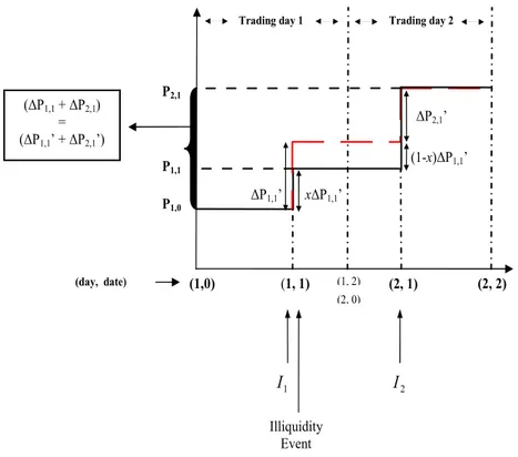
1 I P1,0 2 I Illiquidity Event (1, 1) (2, 1) (2, 2) (1-x)∆P1,1’ ∆P1,1’ (∆P1,1 + ∆P2,1) = (∆P1,1’ + ∆P2,1’) (1,0) (1, 2)

Trading day 1 Trading day 2

(day, date) x_∆P1,1’ ∆P2,1’ (2, 0) P1,1 P2,1

Figure 1: Daily price change as a function of information and liquidity shocks.

Figure 1 illustrates how daily price increment behaves in response to both information shocks and illiquidity events. The dashed lines correspond to the MDH model of Tauchen and Pitts (1983) in which the price moves are a consequence of the new information arrivals. Let ∆P′

1,1 = E1,1P − P˜ 1,0 be the price increment due to I1. As for I1, the trader expectations

concerning ˜P will rise, resulting in a positive ∆P′

1,1. If the market faces illiquidity events

due to the absence of part of the active traders at day 1, the expectation concerning ˜P increases less than if there were no illiquidity problems. In this case, the corresponding price increment is x∆P′

1,1 with x (0 < x < 1) being the proportion of I1 incorporated in the price

change. The day-1-price increment, denoted by ∆P1, is:

∆P1 = x∆P

′

1,1. (2.5)

The corresponding daily traded volume is:

V1 = xV

′

1,1, (2.6)

where V_1,1′ represents the traded volume due to I1. In the absence of illiquidity events, we

should have x = 1, which yields: ∆P1 = ∆P

′

1,1 and Vt= V

′

1,1.

Suppose that no illiquidity event occurs at day 2 and that P2,0 = P1, where P1 = P1,2 =

P1,1 is the price prevailing at the end of day 1. When I2 hits the market, trader’s expectations

concerning ˜P will incorporate I2 and part of I1 that was not incorporated in the previous

trading price (1 − x)I1. The resulting daily price increment, denoted by ∆P2, is:

∆P2 = ∆P ′ 2,1+ (1 − x)∆P ′ 1,1, (2.7) where ∆P′

2,1 reflects the impact of I2 on the daily price change and (1 − x)∆P

′

1,1 is the price

adjustment due to (1 − x)I1. Similarly, the corresponding traded volume is: V2 = V ′ 2,1+ (1 − x)V ′ 1,1. (2.8)

From (2.5) and (2.7) it follows that the price prevailing at the end of day 2, P2 = P2,2 = P2,1,

returns to its fully revealing information level: P2 = P2,0 + ∆P

′ 2,1 + (x + 1 − x)∆P ′ 1,1 = P1,0+ ∆P ′ 1,1+ ∆P ′

2,1. This corresponds also to the price that would prevail in the absence of

illiquidity event at day 1 (as shown by the dashed lines). Thus, the total price change across days 1 and 2 is not impacted by the presence of illiquidity events:

∆P1+ ∆P2 = ∆P

′

1,1+ ∆P

′

2,1. (2.9)

Similarly the total traded volume across days 1 and 2 is:

V1+ V2 = V ′ 1,1+ V ′ 2,1. (2.10) 2.2.2 Generalization Let I∗

t be the number of information arrivals hitting the market at day t that is incorporated

into prices during the same trading day. The "*" symbol indicates that the cumulated impact of information at the daily level may not be entirely incorporated in the daily price changes and volumes. The ith piece of information drives the movement of the market from the (i − 1)th intraday equilibrium to the next (i = 1, ..., I∗

t). Let δi be an indicator variable

taking a value of 1 when an intraday liquidity friction occurs at the ith equilibrium and 0 otherwise. We denote by Lt =

PI∗ t

i=1δi, the number of liquidity frictions occurring at day

t. Let xt (xt ∈ [0 1]) be the proportion of the cumulated daily information impact that is

incorporated in the day-t price increment. More generally, if an illiquidity event occurs at day t, we have I∗

t = xtIt and It+1∗ = It+1+ (1 − xt)It, where It is the number of information

arrivals hitting the market at day t. Since It is considered to be i.i.d., what causes the serial

correlation of It∗ is the occurrence of illiquidity events manifested by xt < 1. It∗ can be

interpreted as the cumulated impact of information arrival and illiquidity events occurrence processes. Henceforth, we will consider I∗

t instead of It in order to capture the dynamics of

daily price changes and traded volumes. The daily price increment can then be written as:

∆Pt = I∗ t X i=1 ∆P_t,i′ + I∗ t X i=1 δi∆P ′′ t,i− I∗ t X i=1 δi∆P ′′ t,i + (1 − xt−1)∆P ′ t−1, (2.11) ∆Pt = xt∆P ′ t + (1 − xt−1)∆P ′ t−1. (2.12) Here, xt∆P ′ t = PI∗ t i=1∆P ′

t,i reflects the impact of It∗ on the daily price change;

PI∗ t

i=1δi∆P

′′

t,i

represents the cumulated price distortion due to the presence of intraday liquidity frictions; −PIt∗

i=1δi∆P

′′

t,i corresponds to price adjustments during intraday GM-processes; and (1 −

xt−1)∆P

′

t−1 represents price adjustment related to the occurrence of an illiquidity event in

the previous trading day. Equations (2.11)-(2.12) generalize the equation (3.29) of Darolles et al. (2010) which is a special case when xt−1 = xt = 1.

Similarly, the daily traded volume equation (4.3.31) can be generalized as:

Vt = I∗ t X i=1 V_i′ + I∗ t X i=1 δiV ′′ i + (1 − xt−1)V ′ t−1, (2.13) Vt = xtV ′ t + V ′′ t + (1 − xt−1)V ′ t−1, (2.14) where xtV ′ t = PI∗ t i=1V ′

i is the daily traded volume due to the information incorporated

in the daily price change; Vt′′ =

PI∗ t

i=1δiV

′′

i is the daily traded volume due to the liquidity

frictions and the intervention of liquidity arbitragers within the trading day and (1−xt−1)V

′

t−1

represents the volume adjustment related to the presence of an illiquidity event at day (t−1). When xt−1 = xt = 1, equation (2.14) corresponds to equation (3.31) of Darolles et al. (2010).

The presence of illiquidity events drives the dynamic properties of the daily price change

and volatility. More precisely, let us consider 2 successive trading days: ∆Pt = xt∆P ′ t + (1 − xt−1)∆P ′ t−1, (2.15) ∆Pt+1 = xt+1∆P ′ t+1+ (1 − xt)∆P ′ t. (2.16)

Assuming that the information arrival and the illiquidity event processes are i.i.d., the dy-namics of daily price change comes from the presence of xt∆P

′

t and (1 − xt)∆P

′

t terms in

respectively equations (2.15) and (2.16):

Cov(∆Pt, ∆Pt+1) = Cov(xt∆P ′ t, (1 − xt)∆P ′ t) (2.17) = xt(1 − xt)V ar(∆P ′ t).

Note that, the covariance between days t and (t+1) depends on the proportion xtof

informa-tion hitting the market at day t that is incorporated in the daily price change. When day-t information is fully incorporated into prices within day t (xt= 1) or is completely reported

to the next day (xt= 0), the covariance between two successive price changes vanishes. For

xt= 1/2 the expression in (2.17) reaches its maximal value. In a similar way, the covariance

between two successive squared price increments can be written as:

Cov(∆P_t2, ∆P_t+12 ) = x2_t(1 − xt)2V ar((∆P

′

t)

2_{). (2.18)}

We now complete our framework by allowing for the latent variable Lt to be

time-persistent. In fact, empirically, several studies, such as Huberman and Halka (1999), Jones (2001), Hasbrouck and Seppi (2001), Amihud (2002), Pastor and Stambaugh (2003) and Acharya and Pedersen (2005) among others, find that liquidity shocks are time-varying and persistent. Intuitively, periods characterized by high (low) liquidity friction occurrence are not isolated events in time but rather seem to extend over several trading days. Since the daily traded volume depends on both information shocks and liquidity frictions, its dynamics

will be impacted by both the occurrence of the illiquidity events and the persistence of the liquidity frictions. More precisely, for two successive trading days, we get:

Vt = [xtV ′ t + (1 − xt−1)V ′ t−1] + V ′′ t , (2.19) Vt+1 = [xt+1V ′ t+1+ (1 − xt)V ′ t] + V ′′ t+1. (2.20)

Assuming that Lt is conditionally independent of It∗, the autocovariance of the daily traded

volume conditional on I∗

t can be decomposed into two components:

Cov(Vt, Vt+1 | It∗) = xt(1 − xt)V ar(V ′ t) + Cov(V ′′ t , V ′′ t+1), (2.21)

where the first term represents part of volume serial correlation due to the occurrence of illiquidity events and the second term is part of volume autocovariance due to the persistence of Lt.

Finally, conditional on I∗

t and Lt, the bivariate mixture (2.1)-(2.2) can be rewritten as:

∆Pt = µpIt∗ + σp p I∗ tZ1t, (2.22) Vt = µatv I ∗ t + µ la vLt+ σv p I∗ tZ2t, (2.23) where I∗

t and Ltare time-persistent and Cov(It∗, Lt| It∗) = 0. Note that, we have introduced

a mean parameter µp in (2.22) in order to account for the presence of serial correlation in

daily price change series as implied by our model in (2.17). Unlike the mean parameters of volume, µat

v and µlav , the µp parameter can be considered as a mean-in-variance parameter

related to the présence of drift effects of I∗

t on price increments at the daily frequency.

In the next section, we exploit the triangular structure of the MDHL model to build a two-step methodology in order to extract dynamic liquidity latent factors using daily time series of returns and volume. To do so, we first use a Markov regime switching stochastic volatility model to extract information shocks I∗

t from the daily price changes. Then, conditional on It∗,

a simple Kalman filter allows us to extract the latent liquidity factor Lt using daily volume

observations. This procedure enables us to: (i) capture the impact of illiquidity events in the daily price change and volatility; (ii) separate the impact of both, the occurrence of illiquidity events and the persistence of liquidity frictions, on the serial correlation of the daily traded volume. As it will be discussed later, the presence of illiquidity events is captured by the coefficient of persistence of I∗

t, while the persistence of liquidity frictions is captured by the

persistence parameter of the latent variable Lt.

3

Methodology

In this subsection we exploit the triangular structure of the extended MDHL model in order to perform time-varying analysis of liquidity problems affecting stock markets. To do so, we first use the stochastic volatility framework to filter the dynamic evolution of the latent variable I∗

t from equation (2.22). Then, a simple Kalman filter applied to volume equation

(2.23) enables us to extract the latent liquidity shocks Lt conditional on It∗ obtained in the

first step.

3.1

A stochastic volatility formulation of price change equation

We now apply the stochastic volatility7

framework to the daily price change equation in order to identify I∗

t. The stochastic volatility formulation of equation (2.22), henceforth SV

model, is given as follows:

∆Pt = µpIt∗+ σp p I∗ tZ1t, (3.1) ln It∗ = β ln It−1∗ + ηt. (3.2) 7

The first-order correlation of squared returns, firstly observed by Mandelbrot (1963), has also been modeled as a generalized conditional heteroscedasticity (GARCH) process (see, for example Bollerslev et al. (1992)). However, as compared with GARCH models, the main characteristic of SV models is that the price change variability is modeled as an unobserved latent variable, which is more in phase with the MDHL framework. Moreover, as discussed by Carnero et al. (2003) among others the SV models capture in a more appropriate way the main empirical properties often observed in daily series of financial returns.

The latent variable It∗ represents the stochastic variance of the daily price change, with β

measuring its persistence. The disturbance of the volatility equation ηt is assumed to be

a gaussian white noise process with mean zero and variance σ2

η, independent of Z1t and

Z2t. Although the assumption of normality of ηt can seem ad hoc at first sight, Andersen

et al. (2001) and Andersen et al. (2003) show that the log-volatility process can be well approximated by a normal distribution. This is coherent with the hypothesis of log-normality of information flow I∗

t made in the MDHL model, which is not new in the literature; Tauchen

and Pitts (1983) assume a log-normal distribution for the mixing variable I∗

t in order to

ensure its positiveness. Log-normality has also been suggested by several authors, such as Clark (1973) as well as Foster and Viswanathan (1993). Richardson and Smith (1994) tested several distribution functions for the information inflow and concluded that the data reject the log-normal distribution less frequently than the other distribution candidates, such as inverted gamma and Poisson distributions. These results motivate us to retain a log-normal distribution for I∗

t.

The SV model given in (3.1)-(3.2) corresponds to the stochastic volatility-in-mean model initially developed by Koopman and Upensky (2002) in order to capture the positive rela-tionship between the expected returns and the the volatility level. In our framework, we explain this positive correlation by the presence of illiquidity events.

(3.1)-(3.2) implies that daily returns and squared returns are serially correlated. Their respective autocovariances are given by:

Cov(∆Pt, ∆Pt+1) = µ2pCov(I ∗ t, I

∗

t+1), (3.3)

Cov(∆Pt2, ∆Pt+12 ) = σ4pCov(It∗, It+1∗ ) + µ4pCov((It∗)2, (It+1∗ )2) (3.4)

+µ2_vσ_p2Cov(I_t∗, (I_t+1∗ )2) + µ2_vσ_p2Cov((I_t∗)2, I_t+1∗ ), (3.5)

where the Cov(f (I∗

t), f (It+1∗ )) (with f (It∗) = It∗, (It∗)2) is a function of the persistence

coeffi-cient β of the shocks to the log volatility. When β > 0, Cov(∆Pt, ∆Pt+1) and Cov(∆Pt2, ∆Pt+12 )

are strictly positive. Thus, to be consistent with the extended MDHL model, we should ex-pect to have β > 0. When µp = 0 the dependence of the daily return sequence appears only

in the squared returns.

We use an iterative procedure to estimate the model parameters and extract the latent variable I∗

t simultaneously. To initialize the procedure, we suppose that µp = 0. Thus

(3.1)-(3.2) reduces to a classical SV model:

∆Pt = σp

p I∗

tZ1t, (3.6)

ln It∗ = β ln It−1∗ + ηt. (3.7)

We use a Markov-regime-switching version of (3.6)-(3.7), denoted by SVMRS model, in order to estimate the model parameters and extract I∗

t, denoted by ˜It∗. The estimation

methodology for the SVMRS model is presented in Paragraphs (5.3.1.1) and (5.3.1.2). Then, we regress the observed ∆Pt on ˜It∗ to estimate µp, denoted by ˜µp. We compute

g

∆Pt= ∆Pt− ˜µp∗E( ˜It∗) for all t = 1, ..., T and apply the SVMRS model estimation procedure

to g∆Pt in order to obtain a new estimation of It∗, ˜It∗(1). The regression of ∆Pt on ˜It∗(1)

yields ˜µp(1). We perform this iteration K times until the change in the mean parameter

value becomes negligable: | ˜µp(K) − ˜µp(K − 1) |→ 0. Finally we use the parameters of this

last iteration and ˜I∗

t(K) as conditioning variables in the volume equation to estimate Lt.

3.1.1 A Markov regime switching stochastic volatility model

The standard SV model (3.6)-(3.7), yields extremely hight levels of persistence. This is useful in practice since estimating or forecasting it becomes easier and estimation errors are smaller. However, the high persistence of volatility may actually arise because of limitations inherent to the AR(1) process assumed for the (log) stochastic volatility in (3.7). This assumption may be too restrictive if there are structural breaks. For example, based on weekly S&P500 index volatility, So et al. (1998) find that volatility is less persistent than

that of SV models. Smith (2002) and Kalimipalli and Susmel (2004) find that, when applied to short-term interest rates, their regime switching models perform better than the GARCH or standard SV models. The motivation behind regime changes in the level of volatility is similar to the jump diffusion stochastic volatility process. Different levels of volatility in stock markets could be attributed, for example, to various political and/or macroeconomic events.

Hwang et al. (2007) generalize the standard SV model in order to account for changes in regime of the level, the variance and the persistence of volatility. They show that the SV models with Markov regime changing outperforms the standard SV and GARCH models. In this study, we apply the Hwang et al. (2007) framework to (3.6)-(3.7) in order to extract the latent variable I∗

t from the observed time series of price changes.

First, linearizing the standard SV model (3.6)-(3.7) by taking logarithms of squared returns yields:

ln ∆P_t2 = ln Z_1t2 + ln σ_p2+ ht,

= µ + ht+ φt, (3.8)

ht = βht−1+ ηt,

where ht= ln It∗, µ = E[ln Z1t2] + ln σp2 and φt = ln Z_1t2 − E[ln Z_1t2] is a martingale différence,

but not normal. Replacing ln ∆P2

t with zt and µ + ht with xt, equation (3.8) can be written

as:

zt = xt+ φt, (3.9)

xt− µ = β(xt−1− µ) + ηt. (3.10)

Then, supposing that there is a state variable st that can assume only {1, 2} values, the

SV model with Markov regime switching equations becomes: zt= xt+ φt, (3.11) xt =                                      µ0+ β(xt−1− µ0) + η0,t, when st= 0, st−1 = 0, µ0+ β(xt−1− µ1) + η0,t, when st= 0, st−1 = 1, µ1+ β(xt−1− µ0) + η1,t, when st= 1, st−1 = 0, µ1+ β(xt−1− µ1) + η1,t, when st= 1, st−1 = 1, (3.12)

where ηi,t ∼ N(0, ση2i) for i = 0, 1 and stfollows a Markov chain with transition matrix given by: p=    p (0,0) _{1 − p}(1,1) 1 − p(0,0) _p(1,1)    , (3.13) with p(i,j)_{= P r(s} t= i|st−1 = j).

Finally, equations (3.11)-(3.12) represent the SV model with Markov regime switching, henceforth SVMRS model. This generalized form comprises the standard8

SV model as a particular case when µ0 = µ1, and σ2η1 = σ

2 η2.

3.1.2 Estimation procedure

We apply Quasi-Maximum Likelihood (QML) estimation method as in Hwang et al. (2007) in order to estimate the SVMRS model parameters as well as the unobserved process xt

from (3.11)-(3.12). In particular, the QML approach for estimating SV models, proposed independently by Nelson (1988) and Harvey et al. (1994) and generalized by Smith (2002) to account for Markov regime switching, is based on the Kalman filter. This is applied to

8

Here, for simplicity, we do not allow for regime changing in the parameter β. A model extension with changes in regime in the persistence of volatility will be investigated in future research.

the logarithm of the observed squared returns zt to obtain one-step-ahead errors and their

variances. These are then used to construct a quasi-likelihood fonction. Because zt is not

Gaussian, the Kalman filter yields minimum mean square linear estimators (MMSLE) of xt

and future observations rather than minimum mean square estimators (MMSE). Although the estimates obtained from the QML may not be as efficient as those obtained by Bayesian methods, such as Markov Chain Monte Carlo (MCMC), or the Efficient Method of Moments (EMM), Broto and Ruiz (2004) show that for large sample sizes the QML estimator behaves similarly to Bayesian estimators.

The log-likelihood function of the SVMRS model (3.11)-(3.12) is:

£_{(z|θp) =} T X t=1 log[f (zt|ℑt−1)], (3.14) where θp = {µ0, µ1, β, ση0, ση1, p (0,0)_{, p}(1,1)_{, σ}2

φ}, ℑt−1 includes all available information at time

t − 1, and f (zt|ℑt−1) is the likelihood function of zt given by:

f (zt|ℑt−1) = 1 X i=0 1 X j=0 f (zt|st= i, st−1 = j, ℑt−1)ξ_t|t−1(i,j). (3.15)

In this equation, f (zt|st = i, st−1 = j, ℑt−1) is the density of zt conditional on st, st−1 and

ℑt−1; under the normality assumption, it is written as:

f (zt|st= i, st−1 = j, ℑt−1) = 1 q 2πF_t(i,j) exp ( −(υ (i,j) t )2 2Ft(i,j) ) , (3.16)

where the mean squared error Ft(i,j) and the prediction error υ (i,j)

t are obtained via the

Kalman filter.

On the other hand, ξ_t|t−1(i,j) in (3.15) represents the filtered transition probability [ξ_t|t−1(i,j) = P r(st = i, st−1 = j|ℑt−1)]; it is updated via the Kalman filter as follows:

ξ_t|t−1(i,j) = p(i,j)ξ_t−1|t−1(j) , (3.17)

with p(i,j)_{being the transition probability and ξ}(j)

t−1|t−1= P r(st−1= j|ℑt−1) being the

condi-tional probability. A more detailed description of the QML estimation procedure applied to SVMRS models is given in the Appendix A.

Once I∗

t estimated, we perform the iterative procedure described previously in order to

obtain ˜µp(K), θp(K) and ˜It∗(K).

3.2

Extracting the intraday liquidity frictions

3.2.1 The state space form of the traded volume equation

The daily volume equation (2.23) can be put in state space form, as follows:

Vt = µatv I ∗ t + µ la v Lt+ σv p I∗ tZ2t, (3.18) Lt = aLt−1+ ωt. (3.19)

The observed daily traded volume Vt is related to the latent factor Lt, known as the state

vector, via the measurement equation ( 3.18). The latent variable Lt is supposed to be

generated by a first-order Markov process given in (3.19), called the state equation. The disturbance ωt is a white noise process with mean zero and variance σ2ω, independent of

Z1t, Z2t and ηt. The state space form (3.18)-(3.19) generalizes the standard MDHL model

assumption that liquidity shocks are serially uncorrelated. The parameter a in equation (3.19) measures the persistence of Lt.

Replacing I∗

t in (3.18) by its estimated counterpart obtained in the previous subsection

and applying the standard Kalman filter to the state space form (3.18)-(3.19) enables us to estimate the volume parameters and extract the latent variable Lt, simultaneously. The

triangular structure of the MDHL model allows us to separate information from liquidity shock impacts on the daily traded volume. Extracting I∗

t and Lt subsequently, provides a

time-dynamic analysis of how the daily traded volume is built up and which type of shocks is responsible for highly traded volume periods.

3.2.2 The estimation procedure We here provide a brief9

summary of the Kalman filter procedure applied to the state space form (3.18)-(3.19) in order to filter Lt conditional on It∗ and estimate the model parameters

accordingly. It is important to distinguish between the hyperparameters θv = {µlav , σv, a}

which determine the stochastic properties of the model and the µat

v parameter associated to

I∗

t which is known. In this case, the term µatv It∗ only affects the expected value of the state

variable Lt and observations in a deterministic way. Since µatv It∗ is a linear function of the

unknown µat

v , this parameter can be treated as a state variable. Let lt = [Lt µatv ]

′

be the state vector. The state space form becomes:

Vt = Ztlt+ ǫt, (3.20)

lt = T lt−1+ Rωt, (3.21)

where Zt = [µlav It∗], ǫ ∼ N(0, Ht) with Ht= It∗σ2v, R = [1 0]

′

, and T is a 2 × 2 matrix given by: T =    a 0 0 1    . (3.22)

Let lt−1|t−1 denote the optimal estimator of lt−1 based on the observations up to and

including Vt−1. Let Pt−1|t−1 denote the 2 × 2 covariance matrix of the estimation error:

Pt−1|t−1 = E[(lt−1− lt−1|t−1)(lt−1− lt−1|t−1)

′

|ℑt−1], (3.23)

where ℑt−1 denotes the information set available up to date (t − 1). Given lt−1|t−1 and

Pt−1|t−1, the optimal estimator of lt is given by:

lt|t−1 = E[lt|ℑt−1] = T lt−1|t−1, (3.24)

9

For more details, see Harvey (2003).

while the covariance matrix of the estimation error is: Pt|t−1 = E[(lt− lt|t−1)(lt− lt|t−1) ′ |ℑt−1] = T Pt−1|t−1T ′ + Rσ2_wR′, (3.25) with σ2

w being the variance of the disturbance wt. Equations (3.24)-(3.25) represent the

prediction equations.

Once the new observation Vtbecomes available, lt|t−1 can be updated using the updating

equations as follows: lt|t = lt|t−1 + Pt|t−1Z ′ tFt−1(Vt− Ztlt|t−1), (3.26) and Pt|t = Pt|t−1− Pt|t−1Z ′ tFt−1ZtPt|t−1, (3.27) where10 Ft = ZtPt|t−1Z ′ t+ H. (3.28)

Taken together (3.24)-(3.27) make up the Kalman filter whose recursive application yields the time series of the state variables lt conditional on θv. Note that, in our theoretical

framework, Lt follows a binomial distribution: Lt ∼ B(p, It∗), with p being the probability

of the occurrence of intraday order imbalances. We here approximate the distribution of Lt

by a normal distribution. In theory, if I∗

t → ∞, and p has the same order of magnitude as

(1 − p), the binomial distribution can be approximated by a gaussian distribution. If this is not the case, we are aware that the Kalman filter yields minimum mean square linear estimators of Lt instead of minimum mean square estimators.

We use the QML method to estimate the model parameters θv. Applying the Kalman

10

It is assumed that the inverse of Ftexists. It can can be replaced by a pseudo-inverse.

filter (3.24)-(3.27) to the observed daily traded volume, we first obtain one-step-ahead errors

(Vt− Vt|t−1) and their variances Ft, which are then used to construct the likelihood function:

log L = −NT 2 log2π − 1 2 T X t=1 log|Ft| − 1 2 T X t=1 (Vt− Vt|t−1)Ft−1(Vt− Vt|t−1), (3.29)

where Vt|t−1 = Ztlt|t−1 is the conditional mean of the observable Vt. Finally, numerical

methods can be used to maximize the likelihood function with respect to the unknown parameters θv.

4

Empirical applications

4.1

The data

Our sample consists in all FTSE100 stocks listed on July 10, 2007. We consider the period from 4 January 2005 to 26 June 2007, i.e., 636 observation dates. We exclude stocks with missing observations ending up with 93 stocks. Daily returns and transaction volumes are extracted from Bloomberg databases. Following Bialkowski et al. (2008), we retain the turnover ratio11

as a measure for volume which controls for dependency between the traded volume and the float. The float represents the difference between annual common shares outstanding and closely held shares for any given fiscal year. Common and closely held shares are extracted from Factset databases.

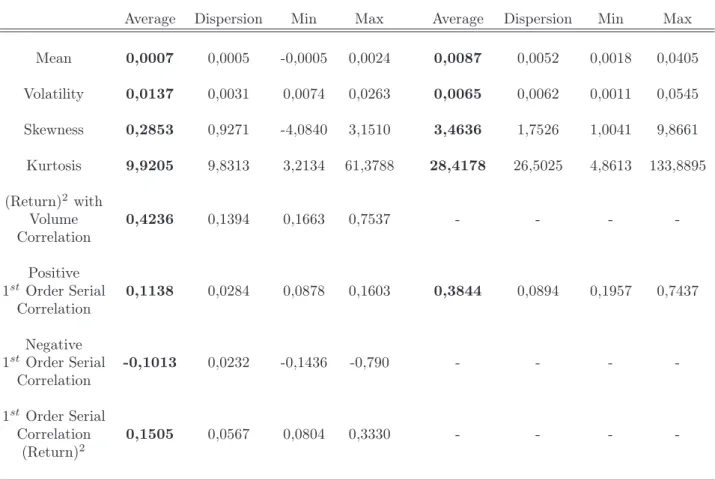
For each of the 93 stocks, we compute: (i) the empirical first moments (mean, volatility, skewness and kurtosis) of volume and returns; (ii) the correlation between squared returns and volume; (iii) the first-order serial correlation of returns, volume and squared returns. The cross-security distribution of these statistics are summarized in Table 1. The first row reports the average, the dispersion, the minimum, and the maximum of the means of returns and volume across the 93 stocks. The second row gives the same cross-section statistics

11

Let qkt be the number of shares traded for asset k, k = 1, ..., K on day t, t = 1, ..., T , and Nkt the float

for asset k on day t. The individual stock turnover for asset k on day t is Vkt=_Nqkt_kt.

Returns Volume

Average Dispersion Min Max Average Dispersion Min Max

Mean 0,0007 0,0005 -0,0005 0,0024 0,0087 0,0052 0,0018 0,0405 Volatility 0,0137 0,0031 0,0074 0,0263 0,0065 0,0062 0,0011 0,0545 Skewness 0,2853 0,9271 -4,0840 3,1510 3,4636 1,7526 1,0041 9,8661 Kurtosis 9,9205 9,8313 3,2134 61,3788 28,4178 26,5025 4,8613 133,8895 (Return)2 _with Volume 0,4236 0,1394 0,1663 0,7537 - - - -Correlation Positive 1st_{Order Serial 0,1138 0,0284 0,0878 0,1603 0,3844 0,0894 0,1957 0,7437} Correlation Negative 1st_{Order Serial -0,1013 0,0232 -0,1436 -0,790 - - -} -Correlation 1st_{Order Serial} Correlation 0,1505 0,0567 0,0804 0,3330 - - - -(Return)2

Table 1: Summary statistics for return and turnover time series.

(average, dispersion, minimum and maximum) of the volatilities of returns and volume, and so on for the skewness, kurtosis, the correlation between squared returns and volume as well as the serial correlation coefficients.

We perform a Pearson test to check the significance of the correlation coefficients com-puted in Table 1. At the 95% confidence level, (i) the squared-return-with-volume correla-tions are statistically significant for 92 over 93 stocks; (ii) the first order serial correlacorrela-tions of returns, volumes and squared returns are significant for 17, 93 and 46 over 93 stocks, respectively. Among the 17 stocks with serially correlated returns, for 11 of them the corre-lation coefficients are negative, leaving us with 6 positive autocorrecorre-lation coefficients. The statistics reported in the 4 last rows of Table 1 are computed using only the statistically

significant coefficients.

The results reported in Table 1 are consistent with the MDHL model. The average and minimum statistics of the volume skewness and squared return correlation with volume are positive; and the average and minimum statistics of return and volume kurtosis are greater then 3, as predicted by the mixture model. In our framework, this positive correlation depends on both information flow and liquidity frictions.

However, the time series of our sample exhibit dynamic properties suggesting that the MDHL model should be extended to account for long lasting liquidity problems. In the next section we confront the implications of the extended MDHL with the sample autocorrelation coefficients. We show that the structural parameters derived by our model improve the naive analysis based on sample autocorrelation coefficients.

4.2

Illiquidity events and momentum strategies

The extended MDHL framework distinguishes between two liquidity problems, the liquidity frictions and the illiquidity events. On the one hand, the liquidity frictions occur at the intraday frequency and increase the daily traded volume while impacting the returns only at the intraday periodicity. These short term liquidity problems are responsible for intraday dynamic properties of returns and volumes12

. Moreover, the persistence of the liquidity frictions explains part of the persistence of the daily traded volume. On the other hand, the long lasting illiquidity events are responsible for the positive serial correlation of daily returns and squared returns. They also explain part of the daily dynamics of the traded volume.

Our two-step methodology exploits the triangular structure of the extended MDHL model (2.22)-(2.23) in order to separate the effects of both liquidity problems using daily time series. More precisely, the first step of our methodology applies a stochastic volatility framework to the daily returns to infer the presence of the illiquidity events. Here, the parameters of

12

Recall that the liquidity frictions results in negative serial correlations for returns and volume and positive serial correlations for squared returns.

interest are µp and β. The second step uses the daily traded volume observations to infer

the presence of the intraday liquidity frictions conditional on I∗

t. Here, the parameters of

interest are µla

v and a.

We now discuss the implications of our results in statistical arbitrage strategies. Actually, the statistical arbitrage traders observe the empirical serial correlation of stock returns and pick up positive serially correlated stocks to build up momentum strategies. Based on the extended MDHL framework, we suggest that the empirical first order serial correlation is not a sufficient criteria to select stocks to be included in these strategies. In particular the tests of significance of the sample autocorrelation coefficients are not appropriate when the observed variables are heteroscedastic. In addition, the sample serial correlation coefficients measure, on average during a time interval, the dependence of returns. A stock may have sample autocorrelations close to zero and still face significant illiquidity events. Their impact on stock returns may be blurred out during a given test period. Therefore, a stock may have a first order serial correlation not significantly different from zero when performing classical test statistics and still be affected by liquidity problems whose presence will be empirically detected using the parameters of our model.

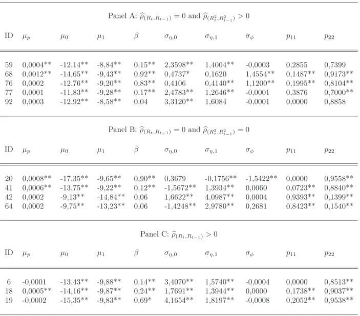
Table 2 in Appendix B reports the estimation results of the stochastic volatility specifi-cation (3.1)-(3.2) for three groups of stocks formed according to their sample autocorrelation coefficients. Let bρ(Rt,Rt−1) and bρ(R2t,R

2

t−1) be the first order sample autocorrelation of returns and squared returns, respectively. Panel A contains stocks with return autocorrelations close to zero but with squared returns significantly serially correlated. Panel B consists of stocks with apparently independent returns. Panel C includes stocks with positive autocorrelation coefficients for daily returns. In the absence of any structural model, an ad hoc momentum strategy would consist in selecting only the third group of stocks13

.

According to our extended framework, the presence of illiquidity events occurring at the daily frequency results in positive autocorrelation of returns and squared returns which is

13

Note that, the case when bρ(Rt,Rt₋₁)<0 will be discussed latter on in this subsection.

captured by respectively the estimated µp and β parameters. Therefore, the model provides

a structural explanation of daily return dynamic properties. The parameters µp and β can

be considered as long lasting illiquidity indicators.

Concerning Panel A of Table 2 in Appendix B, stocks 59 and 68 have µpand β parameters

statistically positive, while their sample return autocorrelations do not differ from zero sig-nificantly. As opposed to the ad hoc analysis consisting of selecting only stock with positive serial correlation of returns, our framework suggests that stocks 59 and 68 should be included in the momentum strategies even if bρ(Rt,Rt−1) = 0 because µp is statistically significant and positive. The ad hoc stock picking strategy should be at least completed by the dynamic properties of the squared returns. In particular, the presence of bρ(R_{2 ,R2}

t−1)

> 0 conveys a favorable signal concerning the presence of illiquidity frictions, whose presence should be then verified using the extended MDHL model. Note also that, the parameter µp allows

identifying appropriate stocks, on average, to be included in the momentum strategies. The variance parameter σ2

p of return equation (3.1), that is captured by the µ0 and µ1 estimated

parameters, provides un idea of risk related to the position held on these stocks. As for stocks 76 and 77, we get µp = 0 and β statistically positive. This means that for these firms,

the serial correlation impact on the daily returns implied by our model does not appear in the observed time series (µp = 0). One possible solution to address this point is to consider

that the daily interval is too large to capture the illiquidity event effects on return dynamics for these stocks. A trading day in the sense of the extended MDHL model should correspond here to less than an effective trading day, say a few hours of trading. This suggests that the appropriate frequency for stocks 76 and 77 to be included in the momentum strategies is smaller than one day. Finally, for stock 92, µp and β parameters are not significant. In

this case the ad hoc stock picking strategy would yield the same results as our structural approach.

Let now consider the panel B of Table 2 in Appendix B. The ad hoc selection strategy based on the sample autocorrelations of returns and even squared returns would not include

these four stocks in the momentum strategies. According to our structural approach, stocks 20 and 41 appear to be affected by illiquidity events since their µp and β parameters differ

significantly from zero. We suggest that these stocks exhibit dynamic properties as captured by µp and β. As for stocks 42 and 64, their structural parameters are not significant. In this

case, our analysis confirms the ad hoc approach results.

The three stocks of Panel C present positive sample autocorrelations for daily returns. According to the ad hoc procedure, these candidates should be included in the momentum strategies. However, only stock 18 has both µp and β parameters significantly positive. As

for stocks 6 and 19, our framework suggests that the day interval is too large to make appear the serial correlation of equity returns. The parameters of our model should be estimates using higher frequency returns.

In our sample there are 11 stocks out of 93 presenting negative autocorrelations of the daily returns; 6 among them has also positive serial correlations of the squared returns. Based on the sample coefficients, the returns of these 6 stocks seem to be driven by a GM-process extending across two successive trading days as discussed in the first paragraph of subsection 2.2. This means that what we call intraday liquidity frictions in this case extend across more than a single effective trading day. Thus, we should expect that at lower frequencies the negative serial correlation should disappear. To illustrate this point, we aggregate for the 11 stocks, their daily returns in order to obtain 2-day returns and then we compute the serial correlation coefficients for these aggregated returns. A the 2-daily frequency the negative serial correlation vanishes for 10 over the 11 stocks.

More generally, the extended MDHL framework provides additional insights concerning the dynamic properties of stock returns. First, by imposing a theoretical structure on the data, we explain the dynamic properties of returns by the presence of illiquidity events. Second, our estimation procedure enables us to infer the presence of the long lasting liquidity problems using the daily time series of equity returns. The illiquidity indicators, µp and

β, represent an alternative criteria in selecting the appropriate stocks in the momentum

strategies. For example, according to the ad hoc approach, only stocks 6, 18 and 19 among the candidates considered in Table 2 in Appendix B should be included in the momentum strategies. Our structural approach helps us selecting some additional stocks such as items 59, 68, 20 and 41. Finally, we suggest that stocks 6 and 19 should be considered with parsimony and that additional tests should be performed, in particular, based on higher frequency observations. The opposite is true for negative serially correlated stocks.

4.3

Intraday liquidity frictions and liquidity arbitrage strategies

The first step of our empirical methodology enables us to estimate µp and β parameters

and filter the latent variables I∗

t simultaneously. Once It∗ extracted using the methodology

described in Subsection 5.3.1, we can filter the latent variable Ltand estimate the parameters

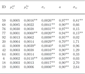
of interest, from the daily traded volume. Table 3 in Appendix C shows the estimated parameters estimated using the specification (3.18)-(3.19). Note that the parameter µat

v is

treated as a state vector which is supposed to converge toward the true value when T is large. We here have reported the last value of the filtered µat

v . The remaining parameters of

interest µla

v, σv, a and σw result from the maximum likelihood estimations.

These procedure completes the standard MDHL framework by accounting for dynamic properties of daily time series. The presence of illiquidity events is captured by the dynamics of the estimated latent factor I∗

t and explains part of the daily volume dynamic properties.

Conditional on I∗

t, we can infer: (i) the impact of intraday liquidity frictions on the daily

traded volume as measured by µla

v and (ii) the the impact of liquidity friction persistence on

the dynamic properties of volume as measures by a. As in the standard MDHL, the µla

v parameter represents the intensity 14

of the liquidity arbitrage trading. However, in our extended framework this indicator is more robust since

14

Note that, the liquidity indicator in the standard MDHL framework is given by pµla

v, where µlav represents

the amplitude of the liquidity arbitrage trading and P the probability of occurrence of the intraday liquidity shocks. The p parameter represents also the expected value of the unobserved Lt factor. In our extended

framework, since we can directly filter Lt, the p parameter can be derived from the sample average of

estimated Lt values.

it take into account the dynamic properties of volume. The results reported in Table 3 suggest that for stocks 59, 77, 41 and 6 the daily traded volume is significantly impacted by trade related to intraday liquidity frictions. These stocks represent liquidity arbitrage opportunities at the intraday frequency. These trading opportunities are a source of trade for the intraday liquidity arbitragers who enter the market to provide the missing liquidity and then liquidate their positions in order to cash the liquidity premium. As discussed by Grossman and Miller (1988), when the liquidity frictions are resorbed rapidly (within the trading day), the expected liquidity premium perceived by the liquidity arbitragers is positive. At the same time, the liquidity premium can be considered as the cost of immediacy for the active traders exchanging against the liquidity arbitragers. Our methodology is thus interesting since it allows: (i) the liquidity arbitragers to detect stocks presenting significant intraday liquidity arbitrage opportunities; (ii) the uninformed traders to detect stocks whose prices deviate from their fundamental values at the intraday periodicity.

Table 3 in Appendix C shows that for all the stocks considered here, the latent variable Lt

is highly persistent. This means that the intraday liquidity frictions are not isolated events in time but can occur during several trading days. As for stocks 59, 77, 41 and 6, with parameter µla

v statistically significant, the liquidity frictions impact significantly the daily

traded volume and explain part of its dynamics which is left unexplained by I∗ t.

More generally, estimating β and a separately allows us to decompose the daily traded volume persistence on two components due to the presence of information shocks and liq-uidity frictions respectively. Our two-step procedure allows us to identify useful stocks for a given trading strategy performed at a given time periodicity. For example, while stocks 59, 68, 20, 41 and 18 should be included at the momentum strategies at the daily frequency, stocks 59, 77, 41 and 6 seem interesting for the short-terms liquidity arbitrage strategies realized at the intraday periodicity.

5

Concluding remarks

In this article, we first distinguish between two liquidity problems, the liquidity frictions and the illiquidity events. The first one impacts stock returns at the intraday frequency while affecting the traded volume at the daily periodicity. The liquidity frictions are a source of trade for the intraday liquidity arbitragers. They also represent the cost of immediacy for the active traders exchanging against the liquidity arbitragers. The illiquidity events represent long lasting liquidity problems and are responsible for daily dynamics of the time series. The illiquidity events represent the risk that liquidity problems may perpetuate and even exacerbate. Second, we extend the MDHL model developed in Darolles et al. (2010) in order to account for the illiquidity events whose presence can be inferred from the daily return dynamics. Third, we exploit the triangular structure of the extended MDHL model in order to separate the impacts of both liquidity problems on stock return and volume dynamics. To do so, we propose a two-step methodology. The first step consists in estimating the illiquidity events from the daily return equation. In particular, we use a Markov-regime-switching stochastic volatility framework in order to filter the impact of information shocks whose dynamics is due to the presence of illiquidity events, I∗

t. In step 2, we apply the

Kalman filter procedure to the daily volume observations in order to infer the presence of the liquidity frictions conditional on the latent variable I∗

t estimated in step 1.

From a theoretical point of view, our extended framework provides a structural inter-pretation of the daily dynamics of returns and volume as well as of the stochastic volatility. From a practical point of view, our estimation results suggest that the sample serial corre-lation coefficients are not sufficient to select the appropriate stocks in building momentum strategies. Our long lasting illiquidity indicators, µp and β provide additional insights

con-cerning the presence of illiquidity problems. In order to compare the relative performances of the sample autocorrelation and structural illiquidity indicators, it would be interesting to back-test two momentum strategies based on each of these criteria. Moreover, the illiquidity indicators proposed here should be computed for more recent periods in order to assess the