This is a publisher-deposited version published in: http://oatao.univ-toulouse.fr/
Eprints ID: 1996
To cite this document: MICHON, Guilhem. BERLIOZ, Alain. LAMARQUE,
Claude-Henri. Experimental and theoretical investigation on nonlinear behavior
of cable-stayed bridges. In: ASME 2009 International Design Engineering
Technical Conferences & Computers and Information in Engineering
Conference, 30 August - 02 Sept 2009, San Diego, USA.
Any correspondence concerning this service should be sent to the repository
administrator: [email protected]
Proceedings of IDETC/CIE 2009 ASME 2009 International Design Engineering Technical Conferences & Computers and Information in Engineering Conference August 30 - September 2, 2009, San Diego, CA, USA
DETC2009-87242
EXPERIMENTAL AND THEORETICAL INVESTIGATION ON NONLINEAR BEHAVIOR
OF CABLE-STAYED BRIDGES.
Guilhem MICHON
Université de Toulouse, ISAE, DMSM,
10 avenue Edouard Belin, 31 055 Toulouse, France
+33 (0)5 61 33 81 58
Alain BERLIOZ
Université de Toulouse, INSA-UPS, LGMT, EA814, 118 route de Narbonne, 31 077Toulouse, France +33 (0)5 61 55 63 75 [email protected] Claude-Henri LAMARQUE
Université de Lyon, ENTPE, Laboratoire Géo-Matériaux
URA CNRS 1652, 3 rue Maurice Audin, 69 518 Vaulx-en-Velin, France
+33 (0)4 72 04 70 75
ABSTRACT
This paper deals with experimental study and with understanding via a finite number of degrees of freedom model of the vibrations of an inclined cable linked to a continuous beam. This is a simplified version of deck and cable of a bridge. External excitation is exerted on the beam. The cable attached to the end of the beam is submitted to a vertical sinusoidal solicitation due to the response of the finite stiffness beam. The excitation of the cable though it is more complex looks similar to the excitation used in previous works. A guided device located at the end of the beam ensures the excitation with a variation of the horizontal component of the cable tension that introduces a new parametric excitation. Analysis of preliminary experimental results for main and secondary resonances permits us to consider simple modeling with one degree of freedom systems obtained by projection of the continuous three-dimensional model of the cable on adapted Irvine mode. Analytical treatment of these models involving data from the experimental devices shows a correct qualitative agreement between preliminary experiments and theoretical. Continuation technique are used to highlight the influence of physical parameters.
INTRODUCTION
Cables oscillations studies have been extensively considered in the past decades. Some of them are devoted to the static behavior [1], as other ones deal with the dynamic aspect [2], [3], [4], with a linear approach. Other work were conducted with the necessary description of the nonlinear
terms to understand the behavior of cables vibration in real environment.
Meirovitch [5] shows that the in-plane motion of a not damped taut cable can be described by a Duffing type equation. Takahashi and Konishi [6] are interested in the free or forced three-dimensional nonlinear vibrations. Benedettini et al. [7], [8], [9] consider oscillations of an elastic cable suspended between two horizontal supports under various cases of resonances. These studies are also important regarding applications (dampers [10], aerial cable-cars [11], tendons control [12], stayed bridges, etc…).
Inclusion of nonlinear terms is compulsory to highlight other phenomenon (nonlinear modal interaction [13], super-harmonic effects, internal resonances [14], bifurcations [15], and parametric nonlinearities [16]). Nayfeh et al. [17] gives some interesting references.
Introducing models with a few degrees of freedom (for example three [18]) is fruitful and permits to explain experimental results.
Gattulli et al. investigates an analytical, numerical and experimental analysis of a cable stayed bridge in [19] and [20]. Their modeling approach is based on the separate description of both medias (i.e. cable and beam), linked by boundary and relevant mechanical conditions.
The results suggested in these multiple references use all the possible approaches to describe, explain but by condensing the phenomenology of the observations. Usually, after the setting in equations in the form of a three-dimensional system
of nonlinear partial derivative equations of evolution governing displacements of the cable, the authors use a discretization by introducing a truncated base of modes of the linear part (Irvine’s modes) selected according to the solicitation range. Projecting on a truncated basis, a regular nonlinear spring – masse system is obtained and studied via analytical methods or by purely numerical approaches according to the type of awaited oscillations.
Usually, the authors considered only horizontal cables. This methodology nevertheless was used by Khadraoui [21] in his PhD thesis on an inclined cable.
The presented piece of research is in the continuity of previous studies [22], [23], [24] in which this method was also used. In this works, the vibrations of an inclined cable were studied from the point of view of two particular resonances: principal resonance where the sinusoidal external excitation frequency is supposed near to the first in-plane Irvine natural frequency, and then when the external excitation frequency is close to the double of the natural frequency. The results obtained showed a good agreement between the experiment and the analytical description obtained for a one degree of freedom system projected on the suitable Irvine’s mode. The adopted analytical method was the familiar multiple scales method.
Nevertheless in this work, the excitation was produced by imposing a displacement directly at the lower end of the cable, with a device that maintained the horizontal component of the cable tension as constant as possible. We considered that this model supposed to represent a small-scale model of a cable-stayed bridge did not truly take into account the deck of the bridge by the introduction of a finite stiffness.
This is the reason why we study here a specific experiment of an inclined cable connected to a horizontal beam. The excitation of the beam is transmitted to the cable via a guidance system constituting an added mass. The measurement of the excitation force permits to decompose the dynamic components of the horizontal reaction and the components of the external excitation transmitted to the cable. The measurement of the excitation exerted on the basis of the cable and the measurement of the response of the cable permits to highlight concerned resonances and to consider a simplified model.
The aim of the paper is to understand by measurement the role of this stiffness, and to use a similar model as simple as possible (ideally a nonlinear one degree of freedoms system), the added beam acting simply like “filters” external excitation. The guidance system acts as a filter for the horizontal reaction to introduce in the simplified model.
The paper is organized as follows: after this introduction, the experimental set-up is detailed in the first Section. The second Section presents experimental results concerning reaction and excitation forces, and specific cable response. The simplified model and its reduction are presented in the third Section. Numerical investigations are carried out in the last Section to highlight the influence of physical parameter on the response amplitude.
EXPERIMENTAL INVESTIGATION Description of the Experimental set-up
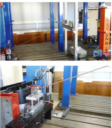
The global experimental set-up, see Figure 1, is composed of a composite flexible blade which represents the deck, and an inclined cable (a steel wire surrounded by copper wire, in order to increase the weight per unit length, but not the flexural rigidity modulus). Both elements are linked to a mass, forced to move vertically, and which represents the anchor point and the equivalent mass of a section of the deck. Therefore, the cable has a given initial static tension due to the mass. A 100N electrodynamics shaker applies a force close to blade clumping. The measurement device is composed as follows. The excitation force from the shaker to the structure is measured thanks to a piezo-electric sensor. The transmitted force from the end of the beam to the mass is also measured thanks to a piezo-electric sensor. The vertical displacement of the mass is measured by a laser displacement sensor. The instantaneous cable tension is measured via an S-shape force sensor, which also captures the static tension. Finally a high resolution laser sensor captures without contact the in-plane motion of the cable.
Push-rods Shaker 100 N θ Laser displacement sensor Laser Micrometer Piezo-electric force sensors Flexible beam
Strain gage Force sensor
Figure 1: Experimental set-up sketch.
Figure 2: Experimental set-up: global view and detail of the excitation system.
Set-up mechanical characteristics and observations
In this experimental device, the cable length is 1.90m, the inclination angle is 21.7°, and the sag is about 10mm. The static tension is adjustable and set in this application to 62N in the cable.
The presence of the beam at the lower end of the cable has an important influence on the natural frequencies of the system. Therefore, if the cable is clamped-clamped, the out of plane natural frequency is equal to 4.87 Hz and the in-plane natural frequency is equal to 6.06 Hz. But, in this case, where the lower end of the cable is linked to a mass and a beam, the out of plane natural frequency is 6.1 Hz, and the in plane natural frequency is 5.8Hz.
Experimental results
The experimental results present the response amplitude of the cable as a function of the excitation frequency for the first two instability zones.
Primary resonance (Ω ≈ω1)
The primary resonance presents a nonlinear behavior even for low excitation amplitude, see Figure 3.
2.7 2.8 2.9 3 3.1 3.2 3.3 3.4 3.5 3.6 0 1 2 3 4 5 6 7
Figure 3: Experimental response amplitude vs. excitation frequency for the in-plane motion of the cable for two
levels of excitation force, for the primary resonance
(Ω ≈ω1), for both sweep directions (* : up; + : down)
Parameters are dimensionless.
Sub harmonic resonance (Ω ≈2ω1)
In the primary parametric instability zone, the response of the cable exhibit large amplitudes, see Figure 4. This instability naturally appears for large excitation amplitudes. A softening behavior is highlighted.
5.9 6 6.1 6.2 6.3 6.4 6.5 6.6 6.7 6.8 6.9 0 2 4 6 8 10 12 14 16 18
Figure 4: Experimental response amplitude vs. excitation frequency for the in-plane motion of the cable for two levels of excitation force, for the sub-harmonic resonance
MECHANICAL MODEL
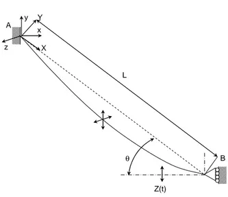
Let consider a cable, of length L, clamped at both ends and inclined of an angle θ with respect to the horizontal axis,
see Figure 5. The motion at the lower end Z(t) is imposed and given by:
( )
01cos( )
Z t =Z Ωt x y X Y L θ Z(t) B A zFigure 5: Inclined cable model.
Classical method consists in considering a nonlinear elastic model of the cable represented by three partial derivative equations system describing the three-dimensional motion of the cable. The different steps are given in [22] or [23].
In our case, and following the experimental observations, the specific boundary condition inverses the classical distribution of in-plane and out of plane natural frequencies. This parameter is essential in the behavior of the response.
Regarding the in-plane vertical observed vibrations, and considering principal nonlinear terms, the retained problem is related to V(s,t), the vertical cable displacement, where t is time and s the curvilinear abscissa identical to the spatial coordinate x. The continuous problem is projected using the following expression for V:
( )
,( ) ( )
. .( )
cos V x t = f x y t +x Z t θwhere y is the unknown modal coordinate, θ the angle of the
inclined cable with respect to the horizontal axis,
( )
cos(
z)
Z t =Z Ω +t φ the imposed displacement at the lower end, and f(x) the Irvine function for the first mode defined by:
( )
0
0 0
0 0 0
1 cos tan sin
2
1 cos tan sin
2 2 2 x x L L f x ω ω ω ω ω ω − − = − −
Static and dynamic deformed shapes of the cable are presented on Figure 6.
Figure 6: Static (dashed) and dynamic (line) deformed shapes of the cable.
Among the parameters governing the obtained equation of motion for the one degree of freedom system, appears the horizontal tension H. This tension is composed of a static part
H0 and a dynamic part rH0, and is written as follow:
(
)
(
)
( )
0 1 cos r cos
H=H −r Ω +t φ θ
Due to the external excitation Z(t), and the moving point B, the damping can be taken under the general form:
(
)
(
)
1 1 c cos1 t c
ξ = ξ + Ω +φ
Where φ φ φZ, ,r crepresent the phase delay between excitation
and displacement, tension and damping respectively.
Finally, the one degree of freedom system which condensed y oscillation is given by:
(
)
(
)
(
)
(
)
(
(
(
)
)
(
)
(
)
(
(
)
)
(
(
)
)
(
)
(
)
(
)
(
)
(
)
(
)
(
(
)
)
(
)
(
)
(
(
)
)
2 2 2 2 2 r 3 3 r 2 1 r z 2 2 2 r z 1 c 0 1 r z 2 3 2 r z 3 r d y dy 2 dt dt y y 1 r cos t y 1 r cos t 1 r cos t Zcos t 1 r cos t Zcos t 1 c cos t 1 r cos t Zcos t1 r cos t Zcos t 1 r cos t
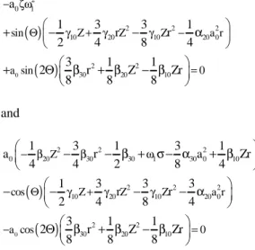
+ ξω + +α − Ω + φ +α − Ω + φ = γ − Ω + φ Ω + φ +γ − Ω + φ Ω + φ + Ω +φ β +β − Ω +φ Ω +φ + β − Ω +φ Ω +φ +β − Ω +φ
Therefore, this model includes a tension fluctuation H, part of
the parametric excitation, and an imposed vertical
displacement Z at the lower end of the cable, responsible for the forcing term in the equation of motion, and also for parametric excitation.
The method of multiple scales in time is used to the first order.
0 1 i i y y y T t,i 0,1 = +ε = ε =
The contribution of nonlinear terms and damping terms are maintained to the same order. So we introduce:
i i 0i i0 i i0 , ,i 1, 2,3 ,i 1, 2 ,i 2,3 β β γ γ ξ ζ = ε = = ε = α = εα = = ε
This leads to the two differential equations:
2 2 0 0 1 2 0 y T y 0 ∂ + ∂ ω =
(
)
(
)
(
)
(
)
(
)
(
)
(
)
(
)
(
(
)
)
(
)
(
)
(
(
)
)
(
)
(
)
(
)
(
)
(
(
)
)
2 2 2 0 1 1 1 2 1 0 0 0 1 1 0 c 0 3 30 0 0 r 2 2 20 0 0 r 10 0 0 r 0 z 2 20 0 0 r 0 z 3 30 0 0 r 2 10 0 r 0 z 20 y T y y 2 T T y 2 1 c cos T T y 1 r cos T y 1 r cos T y 1 r cos T Zcos T y 1 r cos T Zcos T y 1 r cos T 1 r cos T Zcos T 1 r ∂ + ∂ ∂ ω = − ∂ ∂ ∂ − ζω + Ω +φ ∂ −α − Ω +φ −α − Ω +φ +β − Ω +φ Ω +φ +β − Ω +φ Ω +φ +β − Ω +φ +γ − Ω +φ Ω +φ +γ(
−(
)
)
2(
(
)
)
2 0 r 0 z cos Ω +φT Zcos Ω +φT Primary resonanceThe solution of the first differential equation is:
( )
i T1 0[ ]
0 1
y =A T eω + c.c.
Introducing the classical detuning rule:Ω ≈ ω +εσ1 , and eliminating the secular terms in the second differential equation lead to a single complex equation. By using
0 ib 0 a A e 2
= (with a0 and b0 real), and putting Θ = − σb0 T1 , we obtain the two equilibrium equations governing amplitude a0 and phase Θ. They are:
( )
( )
0 2 0 1 2 2 2 10 20 10 20 0 2 2 30 20 10 sin Z Z Z a r a sin 0 a 1 3 3 1 r r 2 4 8 4 3 1 1 2 r Z Zr 8 8 8 − ζω Θ γ + γ γ − = + − − α + Θ β + β − β and( )
( )
0 2 2 2 0 20 30 30 1 30 0 10 2 2 2 10 20 10 20 0 2 2 30 20 10 Z cos Z Z Z a r a cos 0 1 3 1 3 1 a r a Zr 4 4 2 8 4 1 3 3 3 r r 2 4 8 4 3 1 1 2 r Z Zr 8 8 8 − β β ω Θ γ + γ γ − = − − β + σ− α + β − − − − α Θ β + β − β The predicted response amplitude is plotted on Figure 7 for a given set of parameters. The two possible responses merge close to the natural frequency, and move afterwards.
2.950 3 3.05 3.1 3.15 3.2 3.25 3.3 3.35 0.05 0.1 0.15 0.2 0.25
Figure 7: Predicted dimensionless response amplitude vs. excitation frequency, for the primary resonance (Ω ≈ω1).
Sub harmonic resonance
In this case, the detuning rule is:Ω ≈ ω +εσ2 1 and we use
0 1
1
b T
2
Θ = − σ.
The two equilibrium equations are:
( )
( )
2 0 1 2 3 2 0 30 0 30 30 10 20 2 1 1 0 sin 2 a Z Z cos 0 a 1 3 3 1 3 a r r r r 8 16 4 4 16 1 2 c a 2 − ζω + Θ α β − β β − β ζω = − − + + Θ and( )
( )
2 3 2 0 2 2 0 30 10 30 0 30 20 1 2 30 0 30 30 10 20 2 1 1 1 0 3 r 4 3 3 1 3 a 2 r r Z rZ 16 4 4 16 sin 1 3 1 1 1 a Zr a Z 4 8 2 4 2 1 cos a r 4 1 2 c a 0 2 − β − Θ β β β − β + β − α − β − β + ω σ − α − − + + Θ ζ ω =The predicted response amplitude is plotted on Figure 8 for a given set of parameters. Three possible responses exist, where the intermediate solution is unstable.
6.1 6.15 6.2 6.25 6.3 6.35 6.4 0 0.02 0.04 0.06 0.08 0.1 0.12 0.14 0.16 0.18
Figure 8: Predicted dimensionless response amplitude vs. excitation frequency, for the sub-harmonic resonance
(Ω ≈2ω1). NUMERICAL INVESTIGATION
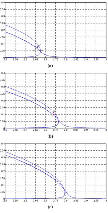
Using continuation technique on the presented model, it is possible to explore the influence of several parameters such as cable static tension, inclination angle, excitation levels, mechanical and geometric properties. In what follow, we
present the influence of the inclination angle on the predicted response amplitude close by the primary resonance, all other parameters being constant. The excitation frequency is, in this case, normalized to a constant value, in order to make the comparison easier.
Even if the shapes of the responses remain identical, it highlights an increase of the response amplitude and frequency versus the inclination angle.
2.5 2.55 2.6 2.65 2.7 2.75 2.8 2.85 2.9 2.95 3 0 0.05 0.1 0.15 0.2 0.25 0.3 0.35 0.4 LP LP LP (a) 2.5 2.55 2.6 2.65 2.7 2.75 2.8 2.85 2.9 2.95 3 0 0.05 0.1 0.15 0.2 0.25 0.3 0.35 0.4 LP LP LP (b) 2.5 2.55 2.6 2.65 2.7 2.75 2.8 2.85 2.9 2.95 3 0 0.05 0.1 0.15 0.2 0.25 0.3 0.35 0.4 LP LP (c)
Figure 9: Predicted (by continuation technique) dimensionless response vs excitation frequency for three
CONCLUSION
This paper was devoted to the experimental and theoretical investigation on the nonlinear behavior of cable stayed bridges. The experimental approach highlighted specific non-linear phenomenon and couplings between the cable and the beam. The softening behavior is due to the presence of the beam stiffness.
The theoretical model is originally based on the classical inclined cables in-plane equation of motion. In the developed model, the cable is both subjected to an imposed boundary displacement and tension fluctuation, which leads to a forced, parametric and nonlinear equation of motion.
Both approaches depict the same conclusion: the cable-beam coupling leads to a softening behavior of the system.
The perspectives are oriented toward the inclusion of the pile stiffness in the model, and also toward the passive control of the phenomenon.
REFERENCES
[1] Krenk S., Mechanics and Analysis of Beams, Columns and Cables, 2nd. Edition, Springer-Verlag, Berlin Heidelberg, 2001.
[2] Irvine H.M., Caughey T.K., The linear theory of free vibrations of a suspended cable, Proceedings of the Royal Society of London, Volume A, 341: 299–315, 1974
[3] Irvine H.M., Cable Structures, The M.I.T. Press,
Cambridge Massachussetts, 1981.
[4] West H.H., Geschwindner L.F., Suhoski J.E., Natural vibrations of suspension cables, J. of the Structural Division, ST11: 2277–2291, 1975.
[5] Meirovitch L., Elements of Vibration Analysis, McGraw-Hill, New-York, 1975.
[6] Takahashi K., Konishi Y., Non-linear vibrations of cables in three dimensions, Part I: Non-linear free vibrations, Journal. of Sound and Vibration, 118 (1): 69–84, 1987. [7] Rega G., Benedettini F., Planar non-linear oscillations of
elastic cables under subharmonic resonance conditions, Journal of Sound and Vibration 132 (3): 367–381, 1989. [8] Benedettini F., Vestroni F., Rega G., Parametric analysis of
large amplitude free vibrations of a suspended cable, International Journal of Solids and Structures 20 (2): 95– 105, 1984.
[9] Benedettini F., Rega G., Alaggio R., Non-linear
oscillations of a four-degree-of-freedom model of a suspended cable under multiple internal resonance conditions, Journal of Sound and Vibration 182 (5): 775– 798, 1995.
[10]Xu Y.L., Yu Z., Non-linear vibration of cable-damper systems Part I: formulation, Journal of Sound and Vibration, 225 (3): 447–463, 1999.
[11]Portier B., Dynamic phenomena in ropeways after a haul rope rupture, Earthquake Engineering and Structural Dynamics 12: 433–449, 1984.
[12]Achkire Y., Active tendon control of cable-stayed bridges, Ph.D., Université Libre de Bruxelles, Faculty of Sciences, 121p, 1997.
[13]Pilipchuk V.N., Ibrahim R.A., Non-linear modal
interactions in shallow suspended cables, Journal of Sound and Vibration 227 (1): 1–28, 1999.
[14]Zheng G., Ko J.M., Ni Y.Q., Super-Harmonic and Internal resonances of a Suspended Cable with Nearly Commensurable Natural frequencies. Nonlinear Dynamics 30: 55–70, 2002.
[15].Reilly O.M, Global bifurcations in the forced vibration of a damped string, International Journal of Non-Linear Mechanics 28 (3): 337–351, 1993.
[16].Lilien J.L,. Pinto da Costa A, Vibration amplitudes caused by parametric excitation of cable stayed structure, Journal of Sound and Vibration 174 (1): 69–90, 1994.
[17]Nayfeh A. H., Pai P. F., Linear and Nonlinear Structural Mechanics, Wiley Interscience, 2004.
[18]Y. Fujino P., Warnitchai B.M., Pacheco, An experimental and analytical study of autoparametric resonance in a 3 DOF model of cable-stayed-beam, Nonlinear Dynamics, 4: 111–138, 1992.
[19]Gattulli V, Lepidi M., Nonlinear interactions in the planar dynamics of cable-stayed beam, International Journal Solids Structures; 40(18): 29–48, 2003.
[20]Gattulli V, Lepidi M, Macdonald JHG, Taylor C. One-to-two global–local interaction in a cable-stayed beam
observed through analytical, finite element and
experimental models, International Journal Non-Linear Mech; 40(4): 71–88, 2005.
[21]Khadraoui I., “Contribution à la modélisation et à l'analyse dynamique des structures à câbles”, Thèse de Doctorat, Université d'Evry, 262p, (in french), 1999. [22]Berlioz A., Lamarque C.H., A Nonlinear Model for the
Dynamics of an Inclined Cable, Journal of Sound and Vibration, 279: 619–639, 2005.
[23]Berlioz A., Lamarque C.H, Nonlinear vibrations of an inclined cable, Journal of Vibration and Acoustics, 127(4): 315–323, 2005.
[24]Boujard O., Pernot S., Berlioz A. and Lamarque C. H., Nonlinear parametric resonances in a stay of the Iroise cable-stayed bridge: analytical model and experiments, Paper DETC2007/MSNDC–35079. Proceedings of the 5th International Conference of Multibody Systems,
Nonlinear Dynamics, and Control, MSNDC-14,