O
pen
A
rchive
T
oulouse
A
rchive
O
uverte (
OATAO
)
OATAO is an open access repository that collects the work of Toulouse researchers and makes it freely available over the web where possible.
This is an author deposited version published in: http://oatao.univ-toulouse.fr/ Eprints ID: 3700
To cite this document: MORLIER, Joseph and YIN, H.P.. On the Robustness of the
Average Power Ratios in Damping Estimation: Application in the Structural Health Monitoring of Composites Beams. In : CST 2010 - The Tenth
International Conference on Computational Structures Technology, Valencia, 14-17 sept 2010
Any correspondence concerning this service should be sent to the repository administrator:
Abstract
In composites structures, cracking, delamination will cause changes in the measured dynamic response of structure and so on experimentally modal parameters. Estimation of damping in structural control often poses a difficult problem especially using broadband experiments. If these estimations are faulty, it is difficult to propose a robust SHM algorithm. Recently H.P. Yin introduced the optimal power ratios damping estimator. A new theoretical basis of the bandwidth method for the damping estimation from frequency response functions (in case of a single degree of freedom system) has been proposed. The main goal of this paper is to study the robustness of this enhanced damping estimator (AIPR) on simulated signal (sampling frequency, Signal to Noise Ratio and damping level/density), and also compare its performance with industrial improved estimator like “Polymax” on experimental FRFs. The pole shifts would be studied as a change in the frequency-damping plane function of level and density of damage.
Keywords: Damping, power ratios, robustness, SHM.
1 Introduction
Since the dynamical behavior of structures is influenced by damage, one is able to detect the occurrence and evolution of damage by monitoring the modal parameters. Besides the detection of structural damage, modal analysis also enables the localization and quantification of the damage since also spatial information is present in the model (mode shapes). Compared to nondestructive testing (ultrasound techniques, analysis of magnetic fields, radiology, thermal methods) vibration-based analysis allows a mixed global/local analysis of the structure with the potential of being applied in situ (laser vibrometer, optical sensor, etc) [1,2]. The investigation focuses in the estimation of damping ratio because among the modal parameters, it is the most difficult to model/estimate. We first analyze the reliability of damping estimation using 2 methods AIPR (Average Inverse Power Ratio) and RFP (Rational Fraction Polynomial) on analytical (supervised) data then we will compare AIPR
Paper 57
On the Robustness of the Average Power Ratios in Damping Estimation: Application in the Structural Health Monitoring of Composites Beams
J. Morlier 1 and H.P. Yin 2
1 University of Toulouse, INSA, UPS, Mines Albi, ISAE, Institute Clément Ader, France 2 University Paris-Est, UR Navier, Ecole des Ponts ParisTech, Marne-La-Vallée, France
results with classical POLYMAX results on benchmark studies of the effect of impact damages on modal parameters on composites and especially thin laminates beams [3-6].In a previous work we study the influence of several parameters on damping estimation [7]: sampling frequency and numbers of spectral lines (which induce the notion of frequency resolution), Signal to Noise Ratio and damping level and density. We compare the robustness and the accuracy of the damping ratio estimation for 3 different methods: RFP, Continuous Wavelet Transform (CWT) and Least Square Complex Exponential (LSCE), RFP robustness even on noisy data have been proved. In experimental data the influence of close modes and/or damping ratio level on the estimation have been highlighted for classical methods that why we wanted to compare our POLYMAX results with new SDOF method like AIPR.
2 Theoretical background
2.1 Tracking of Poles for system identification on FRF
Excellent survey of Experimental Modal Analysis can be found in [8, 9] concerning method of excitation (shaker, hammer etc), types of excitations (burst random, chirp, stepped sine…) and choice of the physical quantity to be measured (displacement, velocity, acceleration). Identification of the frequency-response function (FRF) by means of spectral analysis is usually considered well-investigated. However, currently the choice of the identification parameters (record length, correlation window size, number of averages, etc.) is very subjective and weakly formulated. The choices made are largely empirical and require the experience of a skilled control engineer [10].
The equations of motion for a vibrating structure are commonly derived by applying Newton’s second law :
) t ( f ) t ( x K ) t ( x C ) t ( x
M && + & + = (1)
The excitation forces f(t) and responses are functions of time (t), and M, C, K are the mass, damping and stiffness constants respectively. The equivalent frequency domain form of the dynamic model can be represented with Fourier transforms, as :
) K ) j ( C ) j ( M ( 1 ) j ( F ) j ( X ) j ( H 2 + + = = ω ω ω ω ω (2) Modal parameter estimation is a special case of system identification where the a priori model of the system is known to be in the form of modal parameters. The identification process consists of estimating the modal parameters from Frequency Response Function (FRF) measurements. The current approach in modal identification involves using numerical techniques to separate the contributions of individual modes of vibration in measurements such as frequency response functions.
Each term of the FRF matrix can be represented in terms of pole location and a mode shape: ) ( ) ( ) ( * * k k k k j r j r j H λ ω λ ω ω − + − = (3) Where,
r
k is the (n by n) residue matrix for the kth mode (* designates complex conjugates)k
λ
(Pole value for mode k) = 1 2k k k k
ω
jω
ζ
ζ
+ − − (4)with
ω
k the undamped natural frequency andζ
k the damping ratio of mode k. It has been observed that presence of damage does not affect all the resonant modes equally. A basis for identifying those modes that are affected is therefore necessary for further analysis to pinpoint the damage location. This paper suggests the use of pole shifts as a means for identifying modes affected by damage [11, 12] as impacts create friction zone between plies in the composites.2.2 Rational Fraction Polynomial
The rational fraction polynomial is a SISO frequency domain method [13] and is among the most used nowadays. It is based on the viscously damped model and the FRF is expressed as the ratio of two polynomials:
∑
∑
= − = = N j j j N j j j j b j a j H 2 0 1 2 0 ) ( ) ( ) (ω
ω
ω
(5)A linearized error function is defined between the measured FRF values and the model. Minimizing such an error function, a linear system of equations is obtained, from which the coefficients ak and bk are evaluated (Invfreqs function in matlab
which identify discrete-time filter parameters from frequency response data). The resulting system is usually ill-conditioned. This situation is circumvented by reformulating the problem in terms of orthogonal polynomials. Knowing the resulting coefficients, the modal parameters are retrieved. A global version of this method also exists, i.e. its SIMO version, named global rational fraction polynomial (GRFP), where various FRFs are taken into account simultaneously [14]. A MDOF system is decomposed in the summation of the individual single degree of freedom contributions "SDOF” by residue decomposition (residue function in matlab). Then global parameters are extracted and averaged from every FRF using approximation of equation (4). In this work both methods (MDOF on analytical data, and SDOF on noisy data and experimental data) have been used.
2.3 Power Bandwidth Method and Inverse Power Ratio Method
The classical power bandwidth method [15] for the damping estimation from the amplitude of a FRF is based on the following formula1 2 max − − =
ρ
ω
ω
ω
ζ
b a (6)Where
ω
max is the maximum amplitude frequency,ω
a andω
b are two frequenciesat which the FRF has the same amplitude, ρ is the inverse power ratio defined as
2 2 max 2 2 max
)
(
)
(
)
(
)
(
)
(
)
(
b a b aH
H
H
H
ω
ω
ω
ω
ω
ρ
ω
ρ
ρ
=
=
=
=
(7)Recently, an average inverse power ratio (AIPR) method has been proposed in [16] for the damping estimation by using the following formula
1 2 max − − = + −
ρ
ω
ω
ω
ζ
(8)Where
ρ
is an average inverse power ratio defined at two frequencies situated at the same distance δ fromω
max + + − = 2 max 2 max 2 max 2 max ) ( ) ( ) ( ) ( 2 1
δ
ω
ω
δ
ω
ω
ρ
H H H H (9) a bIn practice, the AIPR method is easier to use than the power bandwidth method which requires data interpolations for the determination of
ω
andω
.3 Supervised numerical simulation
3.1
Supervised damping estimation
This study is carried out on simulated FRF with the aim of identifying the factors which have the most significant effect on damping estimation algorithms [7]. Here we compare AIRP and RFP. The analysis was applied to simulated analytical data set with known properties (Table 1). We can see that the 2 first modes are closed (coupled) whereas the third one is well separated.
Table 1: Pertinent parameters used with analytical data
Natural Frequency (Hz) 318.6 341.1 508.5 Frequency Resolution (Hz) 0.25 0.625 1.5 Damping Level (%) 0.1 0.5 2 Signal to Noise Ratio (dB) 20 30 60
The equation (3) is used to generate analytical FRF using the variables of Table 1 as a sum of decoupled SDOF system.
Our numerical supervised experiments principally focus on the evaluation of AIPR sensitivity against frequency resolution, SNR (White Gaussian Noise). For comparison we added a well established algorithm RFP.
3.2 Damping estimation Vs frequency resolution
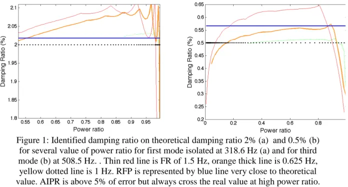
In order to show the Frequency Resolution dependence of the AIPR, 2 examples are shown on figure 1. It reveals as previously implemented (Yin) that the results is better with high frequency resolution and becomes interesting for low damping level (Figure 1). We can see on figure 1 that as damping diminish (peak sharpens) the AIPR method gives better estimation (at better frequency resolution in yellow dotted lines) even than RFP.
Figure 1: Identified damping ratio on theoretical damping ratio 2% (a) and 0.5% (b) for several value of power ratio for first mode isolated at 318.6 Hz (a) and for third mode (b) at 508.5 Hz. . Thin red line is FR of 1.5 Hz, orange thick line is 0.625 Hz, yellow dotted line is 1 Hz. RFP is represented by blue line very close to theoretical value. AIPR is above 5% of error but always cross the real value at high power ratio.
3.3 Damping estimation Vs SNR
In these experiments we use a constant Frequency Resolution of 0.25Hz, and for AIPR interpolation a resolution of 0.1 Hz. The basic principle of our method is to isolate each peak resonance around a bandwidth of 20 Hz for AIPR or RFP.
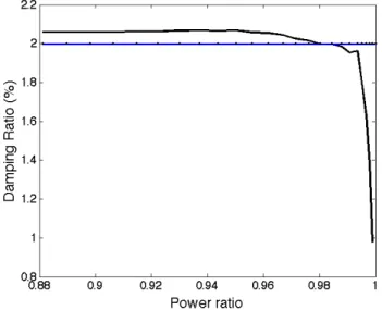
Figure 2: One realization of damping estimation for normal values 2% around the first mode (318 Hz). RFP (thin blue line) gives very good results whereas AIPR (black thick line) gives for low power ratio results around 2.05%. FRF is generated
with a SNR of 60 dB (very low noise).
0.850 0.9 0.95 1 0.5 1 1.5 2 2.5 Power ratio D a m p in g R a ti o ( %) 0.850 0.9 0.95 1 0.5 1 1.5 2 2.5 Power ratio D a m p in g R a tio (%)
Figure 3: Damping estimation (2%) under different realization of a Gaussian noise process (SNR=30dB). RFP is able to fit the analytical model very well and so on
limits the error in damping estimation whereas AIPR is underestimating the damping ratio.
According to 2% damping level tests (Figure 2 and 3), AIPR seems to be more sensitive to noise than RFP SDOF but gives good results (less than 20% errors) for a power ratio zone of 0.85-0.9. At very low SNR (20dB), several trial tests demonstrate (figure 4) that theoretical value is just between an overestimation (RFP) and an underestimation (AIPR). Same kind of results is observed for others modes.
295 300 305 310 315 320 325 -5 0 5 10 15 Frequency (Hz) F R F ( d B ) Noisy Data RFP Data 0.8 0.85 0.9 0.95 1 0 0.5 1 1.5 2 2.5 Power ratio D a m p in g R a ti o ( % ) APR RFP Theoretical
Figure 4: Damping estimation (2%) under different realization of a Gaussian noise process (SNR=20dB). Theoretical value is just in the middle of the 2 estimators
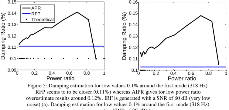
For very low damping level (0.1%), estimators indicate different behaviour. First they become to overestimate the damping ratio (Figure 5).
0 0.2 0.4 0.6 0.8 1 0.09 0.1 0.11 0.12 0.13 0.14 0.15 Power ratio D a m p in g R a ti o (% ) APRRFP Theoretical 0 0.2 0.4 0.6 0.8 1 0.1 0.11 0.12 0.13 0.14 0.15 0.16 Power ratio D a m p in g R a tio ( % )
Figure 5: Damping estimation for low values 0.1% around the first mode (318 Hz). RFP seems to to be closer (0.11%) whereas AIPR gives for low power ratio overestimate results around 0.12%. IRF is generated with a SNR of 60 dB (very low
noise) (a). Damping estimation for low values 0.1% around the first mode (318 Hz) for noisy data (SNR of 20 dB) (b)
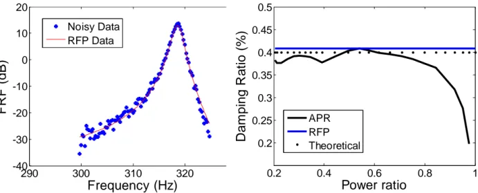
Finally for medium damping level (0.4%) that we are able to observe experimentally on composites materials, our numerical experiments demonstrate (Figure 6) that for very low SNR (noise corresponding to experimental results) AIPR is underestimating the theoretical results.
290 300 310 320 -40 -30 -20 -10 0 10 20 Frequency (Hz) F R F ( d B ) Noisy Data RFP Data 0.2 0.4 0.6 0.8 1 0.2 0.25 0.3 0.35 0.4 0.45 0.5 Power ratio D am pi ng R a ti o (% ) APR RFP Theoretical
Figure 6: Damping estimation (0.4%) under different realization of a Gaussian noise process (SNR=20dB). Theoretical value is just in the middle of the 2 estimators but
the noise has less effect as damping becomes smaller (0.4%)
4 Experimental validation: applications in SHM
4.1 Experimental test rig
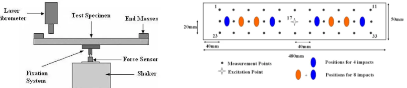
An interesting review of SHM in composites materials could be found in [19]. Vibrations tests for measuring the modal parameters of the composite test specimens and impact tests in order to create damage in the specimens. The experimental set-up is based on Oberst method [18] and states that a free-free beam excited at its centre has the same dynamical behaviour as that of a half length cantilever beam. The test specimen is placed at its centre on a B&K force sensor 8200 which is then assembled on a shaker supplied by Prodera having a maximum force of 100N (Figure 7a). High quality frequency response functions are measured with the help of a Laser Vibrometer OFV-505 provided by Polytec. The centre of the test specimens is excited at Point 17 as shown in figure 7b and a high frequency resolution of (∆f = 0.25Hz) for precise modal parameter estimation. Burst random excitation is used which is a broadband type excitation signal [0-200 Hz]. The signal is averaged 10 times for each measurement point. Hanning windows are used for both the output and the input signals. Response is measured at 33 points that are symmetrically spaced in three rows along the length of the beam (figure 7b). The modal parameters are extracted by a frequency domain estimation method (POLYMAX) based on an automatic extraction using stability diagram.
Figure 7: Experimental set-up for vibration testing (a) and Composite beam specimen with location of damage, excitation and measurement points (b)
The impact test system used to damage the composite beams is drop weight system. The impactor tip has a hemispherical head with a diameter of 12.7 mm. The size of the impact window is 80 x 40 mm2 which allows all the impact points to have the same boundary conditions and all the four ends are clamped.
The five composite specimens [20] are impacted around the barely visible impact damage limit (BVID). BVID corresponds to the formation of an indentation on the surface of the structure, which can be detected by detailed visual inspection and can lead to high damage. In the aeronautical domain, BVID corresponds to an indentation of 0.3 mm after relaxation, aging etc (according to Airbus certifications). Impact energy of 10 J giving an initial indentation depth of 0.55 mm, shall be considered as the BVID limit. We focus on the results of beam 4 on the Table 2.
Table 2 Impact test parameters
Beam No Energy of Impact (J) Height (mm) Velocity of impact (m/s) measured 3 10 (BVID) 552.9 3.24 4 12 663.5 3.52 5 14 774.1 3.84
In fact damage zones are not consistent with the energy of impact even with controlled system we used. Thus it appears local modes in the FRF different for each tested beam, but it is possible to update a finite element with equivalent damage with high correlation using only the first 4 bending modes according to Table 3.
Table 3 Frequency estimation for the first 4 modes versus number of impacts Bending Modes Undamaged 4 impacts 8 impacts 1 41.5 39.8 39.1 2 319.0 308.2 305.1 3 802.1 773.1 760.2 4 1543.7 1477.7 1465.9
4.2 Pole Shift results
Frequency and damping changes are studied with the help of the first four bending modes as they have the largest amplitudes for the type of test configuration presented in this article. As discussed previously, delamination induced damage in composites leads to an increase in damping and a decrease in natural frequency. This effect is more significant in the high frequency range. This fact is verified by our experimental results which show that the difference in natural frequencies between the damaged states (4 and 8) and the undamaged state for the first mode is very small. But this difference in frequencies increases for the higher modes. For the 2nd and 3rd bending modes, the variation of natural frequency as a function of the undamaged (0) and the two damage states (4 and 8) is presented in figure 8.
0 0,1 0,2 0,3 0,4 0,5 0,6 0,7 0,8 0,9 1 39.1 305.1 760.2 1465.9 39.8 308.2 773.1 1477.7 41.5 319.0 802.1 1543.7 Frequency (Hz) D a m p in g R a ti o ( % ) Undamaged 4 impacts 8 impacts
Figure 8 (a) and (b) show that the decrease in natural frequencies with the increase in damage is more significant in case of the higher impact energies. The damping ratios estimated by POLYMAX often tend to increase with impact number.
It can be seen from the results in figure 8 that the damping ratio increases with increase in damage in the beam 4. Others tested beams highlight the same effect. Furthermore, the change in damping ratios between the three states (0,4,8) for the 2nd and 3rd modes is very small whereas frequency shift is clear. However unlike natural frequencies, the increase in damping ratio between the damaged and the undamaged states is not always coherent with the impact energy level, due to the complex nature of damping and the difficulties in its estimation. But in case of Mode 4 damping ratio exhibits quasi linear dependence on the energy of impact.
4.3 Damping Estimation AIPR versus POLYMAX
In order to understand the slight shift in damping ratio for mode 2 and 3 estimate by POLYMAX [21] we analyse the experimental results with AIPR algorithm (isolate each peak resonance around a bandwidth of 20 Hz ) taking 10 random FRFs for mode 1 and 3 random FRFs for mode 2 (very noisy as you can see on Figure 9).
200 400 600 800 1000 1200 1400 -300 -250 -200 -150 Frequency (Hz) F R F ( d B )
Figure 9 Typical FRF with local modes (small peaks) between the 4 first bending modes (higher amplitudes)
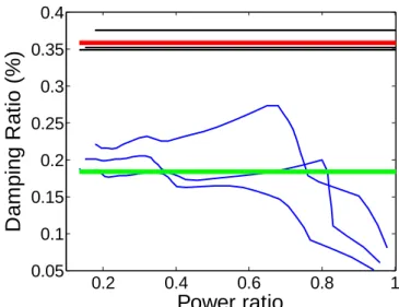
We can illustrate the results using the figure 10: as for medium damping level supervised data, the RFP method overestimates the damping (reference POLYMAX 0.28%) and AIPR method underestimate the reference damping estimation. We can also see that the variance in damping estimation is lower for low power ratio (<0.4).
0.2 0.4 0.6 0.8 1 0.05 0.1 0.15 0.2 0.25 0.3 0.35 0.4
Power ratio
D
am
pin
g
R
at
io
(%)
Figure 10: Damping estimation (undamaged case) using AIPR and RFP for 3 random points on 33 measurements points around 3rd bending mode (800 Hz). The
red line is the average value for RFP (0.358%) and the green line is the average value for AIPR (0.183%) very close to LMS results.
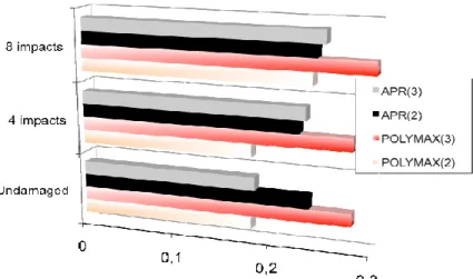
Finally all the results are resumed in figure 11 and globally AIPR (averaged over all the power ratio) results correlate well POLYMAX results and thus these 2 modes are not sensitive to damage comparing to mode 4 where damping ratio exhibits quasi linear dependence on the energy of impact and frequency shift is more important.
Figure 11: Damping estimation (Damping Ratio in abscissa in %) using AIPR and POLYMAX, for different number of impacts.
For engineer one advantage of AIPR is the simplicity: every one knows the classical bandwidth method (Power ratio of 0.5). But here instead of determining the bandwidth for a given value of power ratio which requires numerical interpolations, the method involves an average inverse power ratio calculated at two frequencies symmetrically located from a peak. In this way, the damping estimation from a FRF becomes straightforward for simple modal test cases and would be sufficiently accurate provided that the coupling effects are not strong and the frequency resolution is high enough to determine accurately the peak amplitude frequencies.
4
Conclusion
This paper focuses on the estimation of damping ratio often difficult to estimate accurately. We first analyze the robustness of AIPR method versus classical RFP method using analytical (supervised) data. Our results demonstrate different behaviour function of the damping ratio level. For low damping, low power ratio should be preferred (around 0.3), notably dealing with high noise.
The experimental modal tests aim at showing the effect on modal parameters (pole shift) of multisite localized impacts on composites laminates. We focus especially in 2 modes where the pole shift was not clear using POLYMAX. The simplicity of AIPR method becomes here an advantage for rapid analysis. But the limitation is that a classification of “interesting FRFs” (on the 33 experiments) should be made for a good AIPR estimation (sufficient peak amplitude). We also choose to study the averaged value of AIPR, but it is interesting to see that for low power ratio the variance in the damping estimation is lower. Finally AIPR method well correlates POLYMAX method for noisy experimental data.
References
[1] S. W. Doebling, C. R. Farrar, M. B. Prime, and D. W. Shevitz, Damage Identification and Health Monitoring of Structural and Mechanical Systems From Changes in Their Vibration Characteristics: A Literature Review, LANL Report LA-13070-MS, 1996.
[2] H. Sohn. C.R. Farrar, F. M. Hemez, D. D. Shunk, S. W. Stinemates, B. R. Nadler and J. J. Czarnecki, A Review of Structural Health Monitoring Literature form 1996-2001,LANL Report LA-13976-MS, 2004.
[3] H. Niemann, J. Morlier, Joseph, A. Shahdin, and Y. Gourinat, (In Press: 2010) Damage localization using experimental modal parameters and topology optimization. Mechanical systems and signal processing Volume 24, Issue 3, 636-652,2010.
[4] A. Shahdin, J. Morlier, Y. Gourinat, Correlating low energy impact damage with changes in modal parameters: A preliminary study on composite beams. Structural Health Monitoring, 8: 523-536, 2009.
[5] A. Shahdin, J. Morlier, Y. Gourinat, Damage monitoring in sandwich beams by modal parameter shifts: a comparative study of burst random and sine dwell vibration testing. Journal of Sound and Vibration, Volume 329, Issue 5, 566-584, 2010.
[6] D. Montalvão, N. Maia, A. Ribeiro, A review of vibration-based structural health monitoring with special emphasis on composite materials, The Shock and Vibration Digest ,38, 295-324, 2006.
[7] J. Morlier, B. Chermain and Y. Gourinat, (2009) Original statistical approach for the reliability in modal parameters estimation. In: MAC XXVII A Conference and Exposition on Structural Dynamics, 2009
[8] D.J. Ewins, Modal Testing: Theory, Practice and Applications, 1984.
[9] P. Avitabile, Experimental Modal Analysis – A Simple Non-Mathematical Overview, Sound & Vibration, 2001.
[10] V. Arkova, G. Kulikovb, T. Breikinc, Optimal spectral resolution in system identification, Automatica, 39, 661-668 (8), 2003.
[11] L.D. Mitchell, Modal Test Methods-Quality, Quantity and Unobtainable, Sound & Vibration, 10-16, 1994.
[12] M.H. Richardson and M.A. Mannan, Correlating minute structural faults with changes in modal parameters, Proceedings of SPIE, International Society for Optical Engineering, 1923(2), 893–898, 1993.
[13] M.H. Richardson and D.L. Formenti, Parameter estimation from frequency response measurements using rational fraction polynomials, Proceedings of the International Modal Analysis Conference, 167-181, 1982
[14] M.H. Richardson and D.L. Formenti, Global curve-fitting of frequency response measurements using the rational fraction polynomial method, Proceedings of the International Modal Analysis Conference, 390-397, 1985. [15] H.P. Yin, A new theoretical basis for the bandwidth method and optimal
power ratios for the damping estimation, Mechanical Systems and Signal Processing, 22, Issue 8, 1869-1881, 2008.
[16] H.P. Yin, An average inverse power ratio method for the damping estimation from a frequency response function, Mechanical Systems and Signal Processing, 24, 617-622, 2010.
[17] A.M. Iglesias, Investigating Various Modal Analysis – Extracting Techniques to Estimate Damping Ratio, Master of Engineering, Virginia Polytechnic Institute, 2000.
[18] J.L. Wojtowicki and L. Jaouen. (2004). New approach for the measurements of damping properties of materials using Oberst beam, Review of Scientific Instruments, 75(8), 2569-2574.
[19] Y. Zou, L. Tong,G.B. Steven, Vibration-based model-dependent damage (delamination) identification and health monitoring for composite structures. A review. Journal of Sound and Vibration, 230,357-378, 2000.
[20] A Shahdin, J Morlier and Y Gourinat, Significance of low energy impact damage on modal parameters of composite beams by design of experiments, Journal of Physics: Conference Series,181, 012045, 2009.
[21] B. Peeters, H. V. Auweraer, P. Guillaume, J. Leuridan. The PolyMAX frequency-domain method: a new standard for modal parameter estimation, Shock and Vibrations, 11, 395-409, 2004.