Modèles d'interpolation spatiale et spectrale, anti-crénelage et mesures de qualité

MODELES D'INTERPOLATION SPATIALE ET SPECTRALE,

ANTI-CRENELAGE ET MESURES DE QUALITE

par

Alain Hore

These presentee au Departement d'informatique

en vue de l'obtention du grade de Docteur es sciences (Ph.D.)

FACULTE DES SCIENCES

UNIVERSITE DE SHERBROOKE

Library and Archives Canada Published Heritage Branch Bibliotheque et Archives Canada Direction du Patrimoine de I'edition 395 Wellington Street Ottawa ON K1A 0N4 Canada 395, rue Wellington Ottawa ON K1A 0N4 Canada

Your file Votre reference ISBN: 978-0-494-83313-1 Our file Notre reference ISBN: 978-0-494-83313-1

NOTICE:

The author has granted a

non-exclusive license allowing Library and Archives Canada to reproduce, publish, archive, preserve, conserve, communicate to the public by

telecommunication or on the Internet, loan, distrbute and sell theses

worldwide, for commercial or non-commercial purposes, in microform, paper, electronic and/or any other formats.

AVIS:

L'auteur a accorde une licence non exclusive permettant a la Bibliotheque et Archives Canada de reproduce, publier, archiver, sauvegarder, conserver, transmettre au public par telecommunication ou par I'lntemet, prdter, distribuer et vendre des theses partout dans le monde, a des fins commerciales ou autres, sur support microforme, papier, electronique et/ou autres formats.

The author retains copyright ownership and moral rights in this thesis. Neither the thesis nor substantial extracts from it may be printed or otherwise reproduced without the author's permission.

L'auteur conserve la propriete du droit d'auteur et des droits moraux qui protege cette these. Ni la these ni des extraits substantias de celle-ci ne doivent §tre imprimes ou autrement reproduits sans son autorisation.

In compliance with the Canadian Privacy Act some supporting forms may have been removed from this thesis.

While these forms may be included in the document page count, their removal does not represent any loss of content from the thesis.

Conformement a la loi canadienne sur la protection de la vie privee, quelques formulaires secondares ont ete enleves de cette these.

Bien que ces formulaires aient inclus dans la pagination, il n'y aura aucun contenu manquant.

Lel6decembre2011

lejury a accepte la these de Monsieur Alain Hore dans sa version finale.

Membres du jury

Professeur Djemel Ziou Directeur de recherche Departement d'informatique

Professeur Richard Egli Evaluateur interne Departement d'informatique

Professeur Nizar Bouguila Evaluateur externe

Concordia Institute for Information Systems Engineering Universite Concordia

Professeure Marie-Flavie Auclair-Fortier Presidente rapporteuse

Sommaire

Cette these a publications decrit plusieurs travaux en imagerie, aussi bien au niveau de 1'acquisition des images que du post-traitement des images. Le premier concerne un algorithme de redimensionnement d'images dans lequel le pixel n'est pas considere comme un point, mais comme une unite surfacique exprimee par une fonction mathematique. L'intensite d'un pixel est determinee par interpolation a l'aide des outils du calcul integral. Le deuxieme travail concerne un autre algorithme de redimensionnement d'images dans lequel les derivees de l'image sont mises a contribution pour augmenter le contraste et rehausser les hautes frequences lors du processus de redimensionnement. Pour combiner l'image et ses derivees, nous utilisons le theoreme d'echantillonnage generalise de Papoulis. Dans ce deuxieme travail et dans la suite de la these, le pixel est considere comme un point. Dans le troisieme travail, nous proposons une equation de diffusion aux de'rivees partielles afin de rdduire le crenelage qui apparait regulierement dans de nombreux algorithmes de redimensionnement d'images. L'equation que nous proposons resulte d'un raffinement de l'equation de diffusion de la chaleur utilisee par Perona et Malik. Pour cela, nous introduisons la diffusivite inverse afin de re'duire considerablement le crenelage sur les contours nets. Le rehaussement du contraste pendant le processus de diffusion se fait par 1'integration d'un filtre passe-haut, en l'occurrence le Laplacien, dans notre equation de diffusion. Un modele de reduction efficace du crenelage sur les lignes, base sur les valeurs propres de la matrice hessienne, est egalement propose. Le quatrieme travail est un algorithme de ddmatri§age (ou demosai'cage) permettant de reconstruire une image couleur a partir d'une image acquise par une matrice de filtres couleurs (color filter array, CFA). Sachant que dans un CFA une seule couleur primaire rouge, vert ou bleu est disponible a chaque position de pixel, nous proposons un modele d'interpolation permettant d'estimer les couleurs manquantes a chaque position de pixel. Notre algorithme peut etre utilise pour divers modeles de CFA. II s'inspire

de l'algorithme de dematricage universel de Lukac et al. et y apporte diverses ameliorations. La premiere amelioration est la mise en ceuvre d'une detection de contours ou de zones uniformes dans une image acquise d'un CFA. La deuxieme amelioration concerne 1'utilisation complete du modele de difference des couleurs, qui est un modele bien connu dans les algorithmes de dematricage. La troisieme amelioration est l'utilisation d'un modele d'interpolation spectrale permettant d'interpoler la couleur d'un pixel a I'aide de la couleur et de la position de ses voisins. Dans le cinquieme et dernier travail, nous abordons une problematique liee a la qualite des images, notion importante en imagerie pour la validation des algorithmes et des modeles. Dans notre travail, nous faisons une etude analytique et experimentale pour comparer le PSNR (Peak Signal-to-Noise Ratio) et le SSM (Structural Similarity Index Measure), qui sont deux mesures de qualite largement utilises en traitement d'images. L'etude analytique fait ressortir l'existence d'une relation de type logarithmique entre ces deux mesures. Les nombreux tests experimentaux realises avec differentes images donnent davantage de precisions sur l'efficacite de ces deux mesures a evaluer la qualite des images ayant subi certaines degradations ou traitements tels que la compression Jpeg, la compression Jpeg 2000, le flou gaussien ou le bruit additif gaussien.

Mot cles

Redimensionnement d'images, crenelage, diffusion, dematri5age, detection des contours, mesures de qualite, PSNR, SSIM.

Remerciements

Je remercie le Seigneur Jesus-Christ pour son amour permanent et pour sa grace de tous les jours dans ma vie.

Je remercie mon directeur de recherche, le professeur Djemel Ziou pour la confiance qu'il m'a temoignee, pour l'accueil dans son groupe de recherche, pour son encadrement et son suivi, ainsi que pour le soutien financier dont j'ai beneficie de sa part durant une bonne partie de mes etudes. Ses conseils, son soutien, ses encouragements, ses qualites humaines, son dynamisme, sa disponibilite et sa patience ont joue un role important dans l'accomplissement de ce travail. Qu'il trouve ici, I'expression de ma profonde reconnaissance et de mes sinceres remerciements. Je voudrais egalement remercier le professeur Frangois Deschenes de l'Universite du Quebec a Rimouski, pour les discussions profitables que j'ai eues avec lui et pour son implication dans certains travaux de la these.

J'aimerais remercier mes collegues du centre MOIVRE (MOdelisation en Imagerie, Vision et REseaux de neurones) pour leur sympathie, amitie et collaboration. Je suis heureux de les avoir cotoyes tout au long de ces annees. Je cite particulierement Tayeb Medjeldi, Mohand Said Allili, Sabri Boutemedjet, Samy Metari, Ahmed Fouad Elouafdi, Nadege Rebiere, Ohini Kafui Toffa, Rabia Hammar, Guido Manfredi et Julien Couillaud. Je remercie egalement les membres du jury qui ont accepte de donner de leur temps et pris la peine d'evaluer cette these.

J'adresse aussi mes remerciements a tous les membres de la Mission Rehoboth Internationale / Source de Vie et de I'Eglise Shekina de Sherbrooke, particulierement le Pasteur Pingwinde Baga, le Pasteur Dondon Symphorien, Elisee Miningou et Florent Yamadjoko pour tout leur soutien durant une bonne partie de mes annees de doctorat.

Finalement, je tiens a remercier tous les membres de ma famille pour leur comprehension et pour leurs encouragements.

Table des matieres

Sommaire i

Remerciements iii

Table des matieres iv

Listedes abreviations v

Introduction 1

Chapitre 1 Redimensionnement des images a I'aide des pixels surfaciques 8

Chapitre 2 Redimensionnement des images par le theoreme de Papoulis 25

Chapitre 3 Reduction du crenelage dans les images 42

Chapitre 4 Algorithme de dematricage generique 73

Chapitre 5 Mesures de la qualite des images : relation entre le PSNR et le SSIM

107

Conclusion et perspectives 135

Bibliographic 137

Liste des abreviations

CCD: Charge-coupled device CFA : Color filter array

CIE : Commission internationale de I'eclairage FPGA : Field programmable gate array

MSE : Mean square error

PDE : Partial differential equation PSNR : Peak signal-to-noise ratio RMSE : Root mean square error

SSIM : Structural similarity index measure STD: Standard deviation

Introduction

Au 211&me siecle, force est de constater 1'immersion de plus en plus profonde des images

dans la vie et dans les activites de l'homme. A domicile, dans les environnements de travail et meme en deplacement, un equipement informatique ou un gadget est present pour permettre d'observer ou d'apprecier le contenu d'une scene captee a un moment donne, ou pour extraire des informations a partir du contenu visuel fourni par une image. Au fil des annees, de nombreux modeles, technologies et algorithmes ont ete con§us et mis en oeuvre pour faciliter I'analyse et le traitement des images prises par un capteur. Ainsi, les operations telles que le redimensionnement d'images, le lissage, la detection des contours, le debruitage et la modification du contraste ou de la luminosite ont ete largement etudies a l'aide des theories diverses afin de fournir des images satisfaisantes pour I'analyse et 1'interpretation. La fiabilite de ces differentes operations de traitement est en general evaluee par des mesures de qualite pouvant etre aussi bien objectives que subjectives, c'est-a-dire basees sur des criteres purement mathematiques ou sur la perception humaine. Les capteurs, de leur cote, ont egalement connu un developpement technologique prononce sous divers angles : diminution de la taille des cellules photosensibles afin d'augmenter le nombre de pixels dans les images, reduction du bruit, utilisation des pixels hexagonaux, augmentation de l'efficacite quantique (rapport entre le nombre d'electrons collectes et le nombre de photons incidents sur une surface photoreactive par effet photo-electrique). Aussi, de nombreux nouveaux modeles ont ete proposes pour les matrices de filtres couleurs (color filter array, CFA) recouvrant les capteurs mono-CCD, ouvrant ainsi la voie au remplacement du modele de Bayer [1] encore largement utilise dans les appareils photos par exemple. Contrairement aux capteurs a trois CCD (ou 3CCD) qui permettent d'acquerir simultanement l'intensite des canaux (bandes spectrales) rouge, vert et bleu pour un pixel [2], les capteurs mono-CCD traditionnels ne permettent, pour un pixel donne, que d'obtenir soit la composante du canal rouge, soit la

composante du canal vert, soit la composante du canal bleu. Pour ces capteurs mono-CCD, un algorithme d'interpolation (appele dematricage) doit etre utilise pour retrouver les deux couleurs manquantes a chaque pixel [3, 4], ce qui offre une fiabilite moins elevee que les capteurs 3CCD. Cependant, vu le cout faible des capteurs mono-CCD en comparaison des capteurs 3CCD, de nombreux equipements photos ou videos pour consommateurs sont construits avec des capteurs mono-CCD. Notons toutefois que le Foveon X3 [5, 6] est un modele de capteur CCD dans lequel, a chaque position de pixel, trois photodiodes sont empilees verticalement afin de capter simultanement les composantes des canaux rouge, vert et bleu de la lumiere. Le principe de ce capteur particulier est d'utiliser la propriete selon laquelle les longueurs d'onde de la lumiere penetrent le silicium, qui forme les photodiodes, a des profondeurs distinctes. Ainsi, la profondeur de penetration dans le silicium est caracteristique de la longueur d'onde, et il suffit alors de superposer les photodiodes en mettant plus en profondeur les couleurs avec la plus forte penetration dans le silicium (respectivement, le rouge, le vert, puis le bleu). Dans la suite du texte, les capteurs mono-CCD auxquels nous faisons reference sont ceux pour lesquels une et seulement une seule couleur primaire est disponible pour chaque cellule photosensible.

Dans cette these, nous abordons quatre problemes fondamentaux lies au traitement d'images et a la modelisation des capteurs de pixels: le redimensionnement d'images, la reduction du crenelage, la qualite des images et le dematri§age. Le redimensionnement d'images sera l'objet de deux travaux separes : Fun lie au concept de pixel discret tel que couramment utilise dans de nombreuses recherches en imagerie, et 1'autre lie au concept de pixel surfacique pour se rapprocher de la realite des cellules photosensibles dans les capteurs d'images. Ainsi, un decoupage en cinq chapitres a ete adopte pour la presentation de la these.

Dans le chapitre 1, nous abordons le probleme du redimensionnement d'une image aussi bien sous Tangle de 1'augmentation de la resolution que de la diminution de la resolution. L'objectif d'un algorithme de redimensionnement d'une image est d'augmenter ou de reduire le nombre total de pixels presents dans 1'image. Pour ce faire, un mecanisme est mis en oeuvre pour attribuer des intensites de couleur a des pixels fictifs non presents dans 1'image originale et apparaissant dans 1'image finale. Ce mecanisme peut etre realise de di verses

manieres, les plus en vogue etant 1'interpolation par le plus proche voisin, Interpolation bilineaire et 1'interpolation bicubique. Dans cette these, 1'interpolation qui est utilises dans les algorithmes de redimensionnement ne doit pas etre confondue avec la super-resolution. La super-resolution a pour objectif la reconstruction d'une image de haute resolution a partir de plusieurs images degradees de basse resolution d'une raeme scene [7] (en general, un decalage sous-pixelique est necessaire entre les differentes images de basse resolution afin d'eviter la redondance du contenu des images). En termes d'entrees/sorties, un algorithme d'interpolation a une image en entree et une image en sortie, tandis qu'un algorithme de super-resolution a plusieurs images en entrees et une image en sortie.

Dans ce premier chapitre, le redimensionnement d'images est effectue en utilisant des pixels surfaciques. Ainsi, au lieu de considerer un pixel comme etant un point, nous representons le * pixel par une surface rectangulaire a l'interieur de laquelle l'intensite des couleurs peut etre definie par une fonction mathematique. Dans ce travail, nous explicitons le probleme du redimensionnement d'une image a I'aide des pixels surfaciques et nous exprimons la reconstruction des pixels en utilisant les outils du calcul integral. Le modele que nous proposons pour le redimensionnement des images est une version amelioree du modele propose par Kim et al. [8] dans lequel un pixel est une unite surfacique d'intensite constante. Dans notre modele, un pixel surfacique a une intensite exprimee par une fonction bilineaire. De plus, le nombre de pixels de l'image originale utilises pour interpoler un pixel de l'image redimensionnee depend du facteur de redimensionnement, contrairement au modele de Kim

et al. ou ce nombre est constant.

Dans le chapitre 2, nous presentons un autre algorithme de redimensionnement. Dans les modeles d'interpolation, un probleme recurrent qui apparait est le lissage de l'image et la difficulte a preserver les hautes frequences. Pour resoudre ce probleme, certains algorithmes de redimensionnement sont adaptatifs et utilisent les proprietes locales du voisinage des pixels (par exemple, la detection des contours) pour effectuer une interpolation, non-uniforme dans l'image, qui preserve au mieux les hautes frequences presentes sur les contours et les zones de details [9-11]. Dans le cas des algorithmes de redimensionnement non-adaptatifs (par exemple, replication, interpolation bilineaire, interpolation bicubique), un masque de

convolution constant/uniforme (en general un filtre passe-bas) est utilise sur toute l'image originale pour effectuer 1'interpolation [10]. Par consequent, aucune information locale du voisinage des pixels n'est prise en compte dans ces algorithmes non-adaptatifs et les hautes frequences se trouvent attenuees lors de 1'interpolation uniforme. Afin d'apporter une solution a ce probleme des algorithmes de redimensionnement non-adaptatifs, nous proposons une interpolation, avec masques de convolution, faisant intervenir les derivees de l'image. En effet, les derivees d'une image fournissent des informations sur les hautes frequences. En combinant l'image et ses derivees dans un processus d'interpolation, nous parvenons a obtenir des images moins floues et preservant plus de details que les algorithmes d'interpolation classiques non-adaptatifs. Pour combiner l'image et ses derivees, nous utilisons le theoreme d'echantillonnage generalise de Papoulis [12]. Dans notre modele, nous nous limitons a la derivee premiere et a la derivee seconde d'une image pour effectuer l'operation de redimensionnement. Des derivees d'ordres superieures peuvent aussi etre utilisees, mais elles donnent lieu a plus de calculs sans forcement augmenter de maniere significative la qualite des images. Le modele du pixel utilise dans ce chapitre et dans la suite de la these est le pixel-point.

Le chapitre 3 est consacre a la problematique du crenelage dans les images. En traitement du signal, le crenelage fait reference a un effet qui rend indifferenciables, au moment de l'echantillonnage, deux signaux pourtant differents [13]. Plus specifiquement en traitement d'image, le crenelage se presente sous la forme d'images grossierement pixelisees dans lesquelles les contours apparaissent avec des effets d'escaliers au lieu d'etre lisses. Le phenomene du crenelage se retrouve frequemment dans les algorithmes de redimensionnement d'images et il est particulierement visible dans l'algorithme utilisant 1'interpolation par le plus proche voisin [14]. Pour reduire le crenelage, des filtres passe-bas peuvent etre utilises pour effectuer des operations de lissage afin d'uniformiser au mieux les pixels presentant des effets de pixelisation ou d'escaliers. Cependant, les filtres passe-bas creent beaucoup de flou puisqu'ils sont appliques sur toute l'image indifferemment des particularites de certains pixels qui peuvent etre des points de contours ou de hautes frequences. Pour attenuer cet effet de flou, des methodes de diffusion peuvent etre utilisees

afin d'effectuer un lissage selectif des pixels. Dans ce travail, nous proposons une equation aux derivees partielles pour effectuer la diffusion dans une image presentant des effets de crenelage. Notre equation est un raffinement de V equation de diffusion de Perona et Malik [15], a travers notamment un changement subtil de la diffusivite. En effet, nous avons observe que, avec le coefficient de diffusivite tel que utilise dans le modele de diffusion de Perona et Malik, le crenelage sur les contours n'etait pas proprement reduit. Pour resoudre ce probleme, nous utilisons ce que nous appelons la diffusivite inverse. II s'agit d'une reecriture de la diffusivite pour permettre une meilleure diffusion dans les zones de gradient eleve, caracteristique du crenelage, tandis que les autres zones sont moins concernees par la diffusion. Afin d'augmenter le contraste et reduire la perte des hautes frequences engendrees intrinsequement par la diffusion, nous proposons un modele general de diffusion dans lequel un filtre haut est utilise. Dans le cas de nos applications experimentales, le filtre passe-haut est donne par le Laplacien. Un probleme que nous rencontrons avec notre modele ainsi defini est la faiblesse de la reduction du crenelage dans le cas des images contenant des lignes, ce qui est principalement du a un mauvais coefficient de diffusivite utilise pour le cas des lignes. En effet, certaines etudes ont revele que le gradient n'est pas un bon estimateur pour la determination des lignes [16, 17] et que de meilleures estimations pouvaient etre obtenues en utilisant les valeurs propres de la matrice hessienne. Ainsi, pour reduire efficacement le crenelage dans les images contenant les lignes, nous redefinissons le coefficient de diffusivite pour qu'il ne se calcule plus a partir du gradient comme dans le modele de Perona et Malik, mais en utilisant les valeurs propres de la matrice hessienne correspondant a l'image.

Dans le chapitre 4, nous abordons le dematricage qui est un probleme recurrent rencontre dans les capteurs mono-CCD contenant un seul CFA. En 1976, Bayer a propose un modele de CFA dans lequel il y a deux fois plus de pixels verts que de pixels rouges ou bleus [1]. Cette configuration a ete adoptee pour se rapprocher des caracteristiques du systeme visuel humain qui est plus sensible au vert qu'au rouge ou au bleu. Depuis maintenant quelques annees, on assiste a une explosion de modeles de CFA dans lesquels differentes configurations et agencements des pixels sont proposes [18-21]. Sachant qu'un CFA est

caracterise par le fait qu'une seule des couleurs primaires rouge, vert ou bleu est disponible a la position d'un pixel donne, un element essentiel a la validation d'un CFA est l'algorithme de dematrigage utilise pour interpoler les deux autres couleurs primaires manquantes a la position de chaque pixel. Au fil des annees apres l'apparition du modele de Bayer, un grand nombre d'algorithmes de dematrigage ont ete proposes et continuent d'etre proposes pour le modele de Bayer [22]. En 2005, Lukac et al. ont propose un algorithme universel pour le dematrigage des CFA composes de pixels rouges, verts et bleus [23]. Cet algorithme, bien que performant sur des images relativement uniformes, apparait moins fiable pour gerer efficacement les contours dans les images. Fort de ce constat, nous proposons un modele de dematrigage qui s'inspire du modele de Lukac et al. et qui l'ameliore a travers trois apports essentiels. Premierement, nous integrons un mecanisme de detection des zones uniformes et des contours permettant, aux points de contour, d'interpoler dans la direction du contour et non a travers le contour, ce qui reduit les problemes de crenelage ou de fausses couleurs. Deuxiemement, nous proposons un modele d'interpolation spectrale qui s'inspire du principe du centre gravite et qui favorise une interpolation selon laquelle I'intensite d'un pixel depend non seulement de I'intensite de ses voisins, mais aussi de leur position dans le voisinage. Troisiemement, nous implementons completement, et non partiellement, le modele de difference des couleurs couramment utilise dans les algorithmes de dematrigage pour simuler la propritete selon laquelle, dans les regions homogenes, la difference entre les pixels de deux canaux (rouge, vert ou bleu) est relativement uniforme [24]. Pour conclure ce travail, nous etablissons le lien entre le dematrigage et le redimensionnement des images et nous explicitons un processus permettant, a partir de notre algorithme de dematrigage generique, d'effectuer le redimensionnement d'une image.

Dans le chapitre 5, nous abordons la problematique des mesures de qualite d'images. Plus specifiquement, nous faisons une etude comparative analytique et experimentale du PSNR (peak signal-to-noise ratio) et du S S M (structural similarity index measure) [25], qui sont deux mesures de qualite d'images largement utilisees en imagerie. La motivation premiere derriere ce travail vient d'un evaluateur d'un article que nous avions soumis a une revue. Cet evaluateur n'etait pas tres en accord avec le fait que nous ayions utilise le SSIM

pour comparer des images et il nous recommandait d'utiliser le PSNR. Pour repondre plus specifiquement a l'evaluateur, et afin d'apporter a la communaute scientifique une meilleure connaissance du PSNR et du SSIM pour l'analyse et 1'interpretation des resultats de ces mesures, nous proposons une etude dans laquelle les points de similarity et de difference entre le PSNR et le SSIM sont abordes. Pour ce faire, nous revisitions les formules du PSNR et du SSIM et nous degageons une relation analytique logarithmique entre ces deux mesures qui est valable pour des operations de traitement d'images dans lesquelles il y a conservation de la moyenne des images (par exemple la compression Jpeg, la compression Jpeg 2000, le lissage gaussien, l'ajout de bruit additif gaussien de moyenne nulle). De maniere surprenante, cette relation analytique met en lumiere l'existence d'une linearite partielle entre le PSNR et le SSIM. Par ailleurs, cette relation permet d'expliquer le fait que deux images degradees puissent avoir la meme valeur du PSNR mais deux valeurs differentes du SSIM comme observe experimentalement [26], et vice-versa. Dans ce travail, nous expliquons egalement certains resultats observes sur la haute performance du PSNR dans 1'evaluation des images contenant du bruit additif gaussien [27]. Dans un cadre plus large, nous abordons une etude experimentale de la sensibilite du PSNR et du SSIM en fonction des changements de parametres caracterisant certains traitements (bruit additif gaussien, compression Jpeg, compression Jpeg 2000, lissage gaussian). Cette etude experimentale permet de faire ressortir les types de traitement d'images pour lesquels il serait approprie d'evaluer objectivement la qualite des images en utilisant soit le PSNR, soit le SSIM ou les deux.

Chapitre 1

Redimensionnement des images a Paide des pixels

surfaciques

Dans ce chapitre, nous proposons un algorithme de redimensionnement permettant d'augmenter ou de reduire la resolution d'une image en utilisant des pixels surfaciques. Ainsi, au lieu de considerer un pixel comme etant un point, nous representons le pixel par une surface rectangulaire a l'interieur de laquelle l'intensite des couleurs est definie par une fonction mathematique. Le but de cette representation est de se rapprocher de la realite physique des cellules photosensibles qui sont en fait des unites surfaciques et non des points. Sur la base de cette representation, nous nous rapprochons des images continues, ce qui offre beaucoup plus d'informations sur les images ainsi qu'une plus grande souplesse pour la visualisation, 1'interpolation et le traitement des images. Le travail presente est une amelioration du modele propose par Kim et al. [8] dans lequel un pixel est une unite surfacique d'intensite constante. Pour ce faire, nous commen?ons par expliciter le probleme du redimensionnement d'une image a l'aide des pixels surfaciques et nous exprimons la reconstruction des pixels en utilisant les outils mathematiques du calcul integral. Dans notre modele, un pixel surfacique a une intensite exprimee par une fonction bilineaire, ce qui apporte une meilleure precision sur le calcul de l'intensite des pixels par rapport au modele des pixels surfaciques constants. De plus, le nombre de pixels de I'image originale utilises pour interpoler un pixel de I'image redimensionnee depend du facteur de redimensionnement, ce qui augmente I'efficacite de 1'interpolation contrairement au modele de Kim et al. ou ce nombre est constant.

Nous presentons, dans les pages qui suivent, un article intitule A Simple Scaling Algorithm Based on Areas Pixels qui est paru dans les actes de International Conference on

Image Analysis and Recognition (ICIAR), Povoa de Varzim, Portugal, 2008 [28]. Le

probleme a ete pose par les professeurs Djemel Ziou et Francois Deschenes. J'ai realise, valide et redige ce travail sous la supervision du professeur Djemel Ziou.

A Simple Scaling Algorithm Based on Areas Pixels

Alain Hore, Francois Deschenes, and Djemel Ziou

June, 2008

Abstract. In this paper, we propose a new scaling algorithm which performs the scaling up/down transform using an area pixel model rather than a point pixel model. The proposed algorithm uses a variable number of pixels of an original image to calculate a pixel of the scaled image. Our algorithm has good characteristics such as fine-edge and good smoothness. Different quality parameters (standard deviation, root mean square error, aliasing, edge map) are used to compare our algorithm with four image scaling algorithms: nearest neighbour, bilinear, bicubic and winscale algorithms. The results show that our algorithm generally produces images of better quality with few aliasing, few blur and high contrast.

Keywords: Resizing, scaling, area pixel, standard deviation, mid point rule.

1 Introduction

Recently, the digitization of images has got a great interest in the transmission, processing and storage of the image data [8]. In fact, digital display devices such as liquid crystal display (LCD) or plasma display panel (PDP) that directly use digital data in displaying images are now very popular. While the resolutions of image sources are various (e.g., VGA, SVGA, XGA, SXGA), the physical screen resolution of a digital display device is fixed. In the case where the resolution of a stream image generated by a host PC is different from the screen resolution of a digital display device, an image-scaling process is necessary [10]. In the image-scaling process, image quality should be preserved as much as

possible. The basic concept of image scaling is to resample a two-dimensional function on a new sampling grid [15], [16]. During the last years, many algorithms for image scaling have been proposed. The simplest method is the nearest neighbour [5], which samples the nearest pixel from original image. It has good high frequency response, but degrades image quality due to aliasing. A widely used method is the bilinear algorithm [6]. In bilinear, the output pixel value changes linearly according to sampling position. There is also a more complex method called bicubic algorithm [8]. The weakness of bilinear and bicubic is the blur effect causing bad high frequency response. Recently, many other methods using polynomial [1], [18], adaptive [2], [17], connectivity [13], sampling [7], compression [14], or correlative properties [11] have been proposed. However, these methods have complex representations which imply excessive computations. In another method [3], the scale ratio is fixed at powers of two. It prohibits the method from being used in screen resolution change requiring a fractional scaling ratio. Most of the algorithms consider the pixel in the CCD sensor as a single point corresponding to a sampled location. This has the advantage of simplifying the description of an image and reducing the complexity of algorithms. However, the point-pixel model does not simulate the physic of the photosensitive cells which are represented by rectangular areas. In order to simulate the physic of the photosensitive cells in the CCD sensors, Ziou et al. [19] proposed a new image model where images are globally described in n dimensions by n-cubes called n-pixels. For example, when n=0, the image is a set of points; when n=l, set of edges, and when n=2, a set of rectangular areas. The advantage of this model is that it allows to represent pixels and to describe images by an algebraic formalism. Also, the image dimension is explicit, which allows to design algorithms that operate in any dimension. In this paper, we are interested in the case of 2-pixels which are globally called areas pixels. Very few works have been proposed on image processing algorithms based on areas-pixels. In [9], Kim et al. introduced a new resizing algorithm called winscale in which pixels are considered as areas of constant intensity. Their algorithm generally gives images of good quality but imposes many assumptions: in the scaling down process for example, the algorithm executes differently and often not in an optimal way depending on the scaling ratio (greater or smaller than 2); also, in the scaling up process, the algorithm works differently

depending on the scaling ratio (an integer number or not). Those different aspects of the winscale algorithm stem from the fixed number of constant areas-pixels of the original image that are used to compute the mean grey level of an area-pixel of the scaled image. Also, the authors did not define a precise mathematical model which describes an area pixel.

In this paper, we introduce a new image scaling algorithm which uses the area coverage of the original pixels of an image for computing the pixels of the scaled image. We propose a mathematical model for describing the areas-pixels and computing their grey levels. Our algorithm can be seen as a generalization and improvement of the winscale algorithm. The outline of the paper is organized as follows: in Section 2, we give a description of the area-pixel for the scaling algorithms. In Section 3, we present our scaling up algorithm based on areas-pixels. Section 4 describes the scaling down algorithm. In Section 5, we present the experimental results. We end the paper with the concluding remarks.

2 Basic concept of areas pixels

Basically, our algorithm uses an area pixel model and a domain filtering method for image scaling. The concept of area-pixel is tightly related to the image acquisition process inside sensors. CCD sensors are made of photosensitive cells which store up light during a certain time (exposure time); the value attributed to a pixel is proportional to the amount of light received at one point of the cell. In the classic model, the amount of light at one point is used to represent the entire cell in which it is located. In the area-pixel model, a cell is no longer represented by a single point, but by a function describing a surface. Very few authors have addressed the concept of areas-pixels so far; however, we note that Chan et al. [4] and Molina et al. [12] used a simple area-pixel model for the super-resolution problem: they considered pixels as areas of constant intensity and they derive effective algorithms. In our algorithm, the pixel shapes of the original and the scaled images are treated as rectangles. In the case of areas-pixels of constant intensity, the intensity is evenly distributed in the rectangles areas. For this first work, we assume that the intensity of an area-pixel is described by a 2D polynomial of degree 1 (bilinear polynomial); this assumption offers a simple but more general representation of areas-pixels. Other functional representations (wavelets,

higher degree polynomials, etc.) are possible, but they are not discussed in this paper. In Figure 1, w e show an area-pixel and its four corners points represented b y a f u n c t i o n / . L e t ' s consider the model of area-pixel described b y a 2 D polynomial of degree 1. T h e n , every point

(x,y) inside a pixel has the following intensity:

f(x, y) = ax+by + cxy + d, a,b,c,deR (1)

/[>,;

/[.+U]

/ ( « )

/ K J + 1 ]

/['*I,J*I]

Figure 1: A n area-pixel represented b y a f u n c t i o n / .

Inside a pixel (ij), w e obtain the coefficients a, b, c and d b y solving the following system:

j V 5 + 1 j (' + 1)7 1 7 + 1 i(j + l) 1 + 1 y + 1 0 + l ) ( j + l) l) VflN b c

/ M 1

We suppose that the value/[/j] is the intensity at the top-left point of the pixel (ij). Solving (2) yields:

f(x,y) = alf[i,j]+a2f[i + \,j] + a,f[i,j+l]+aj[i + \,j+\]

a,=(l + i-x)(l + y - y ) a2=(x-i){\ + j-y) a,={\ + i-x)(y-j) a4=(x-i)(y-j) (3)

3 Scaling up algorithm

W e consider each pixel of the original and the resized image as an area. Given an original image d e c o m p o s e d into a number of areas corresponding to its size, w e want to c o m p u t e the mean grey level of the areas-pixels of the scaled u p image. T h e width and height

of the new areas-pixels are determined by the scale factors (we suppose that the width and height of the areas-pixels of the original image are equal to 1.0). For example, if the scale factor is 2.5x2, then each area-pixel of the resized image is of size 0.4x0.5. Figure 2 shows the areas-pixels of an original and the resized image. Each pixel of the resized image can be in four different configurations inside the pixels of the original image.

" " " " T ; • • *

• » » • . . • . . » • . .

l*lt»IMI»lt1MIMM

! 1 J I Pixel of the original image • : Pixel of the resized image

Figure 2: The areas-pixels of an original and a resized image.

The different configurations are illustrated in Figure 3. The mean intensity of an area-pixel of the resized image is obtained by computing the integral of the image in the domain covered by that area-pixel. As we have four configurations of the pixels (see Figure 3), we also have four cases to consider for computing the mean intensity of an area-pixel of the resized image: Case 1: an area-pixel of the resized image is entirely included in an area-pixel of the original image (Figure 3.a)

Let's denote by AooOfo,yo) and Au(x\,yi) the top-left and bottom-right corners delimitating the pixel of the resized image. Then, the mean grey level (mean intensity) GL of the area-pixel of the resized is given by:

1 *> y> (4)

If/is described by a polynomial of degree 0 or 1, then the integral appearing in (4) can be exactly computed without any error term by using the midpoint rule. We recall that the midpoint rule states that:

4»(w.) ~ A..^.,AI A?( W l ) 4 : ( W : ) J & » 4u ( *i- yi' (a) Configuration 1 ^ \

,AA\

7 \

• : Pixel of the resized image

Figure 3: Configuration of an area-pixel of the resized image among areas-pixels of the original image.

]f{x)dx = {b-a)f

a + b) {b-af

,

24

\3r»

The error term {b-a)'f\e)l2A is zero (that is, the integral is exact) when the function / is a polynomial of degree 0 (constant) or 1. Consequently, we can rewrite (4) as :

GL =

(«-*)(*-*)/ *f*.*f*

(6)

/ •*>+•*! y» + yi

(xi-xa){yi-yo)

In the case of a 2D polynomial of degree 1, each term f(x,y) can be computed by using (3). In the simple case of area-pixel of constant intensity, j{x,y)=j[int(x),int(y)] (int denotes the integer part).

Case 2: an area-pixel of the resized image crosses the vertical border of two areas-pixels of the original image (Figure 3.b).

Let's denote by Aij{xi,y}), i e {0,1}, j e {0,1,2} the six points delimitating the intersection

between the area-pixel of the resized image and the two areas-pixels of the original image as illustrated in Figure 3.b. The mean grey level GL of the area-pixel of the resized image is given by: i y\ (7) GL = (x,-x0)(y2-y0)H 1 \\f{x,y)dxdy (x<-Xo)(yi-y«)

By using the midpoint rule, we obtain:

\\f(x,y)dxdy+\]f(x,y)dxdy

+ (*-*)/ * f ^

We note that if S(ij) is the top-left point of the first original area-pixel containing a part of the area-pixel of the resized image we are computing, then y\=j+l (we recall that the width and height of each area-pixel of the original image are considered to be equal to 1.0).

Case 3: an area-pixel of the resized image crosses the horizontal border of two areas-pixels of the original image (Figure 3.c).

Let's denote by A,y(x,,yy), i e {0,1,2}, j e {0,1}the six points delimitating the intersection between the area-pixel of the resized image and the two areas-pixels of the original image as illustrated in Figure 3.c. The mean grey level GL of the area-pixel of the resized image is given by: 1 Yi . (9) GL = (Jf2-J£b)(3'i-3'o)iv \\f{x,y)dxdy «0 >D {x2-x0)(yy-y0) Jo V,

j jf(x,y)dxdy+ J jf(x,y)dxdy

By using the midpoint rule, we obtain 1 GL = -x2 xu ( * | - * o ) / ' * , + * , y 0 + y^ + {*2-Xl)f x,+x2 y„ + yt (10)

We note that if S(iJ) is the top-left point of the first original area-pixel containing a part of the area-pixel of the resized image we are computing, then JCI=/+1 .

Case 4: an area-pixel of the resized image is at the intersection of four areas-pixels of the original image (Figure 3.d)

Let's denote by A,j(x„yj), i e {0,1,2},,/' e {0,1,2} the nine points delimitating the intersection of the area-pixel of the resized image and the four areas-pixels of the original image as illustrated in Figure 3.d. The mean grey level GL of the area-pixel of the resized image is given by: (11) GL = {xi-xo){y2-y0)i;

j Jf(x,y)dxdy

I I J \f{^y)dxdy

{x2-

o){yi-yo)tzU: ;

By using the midpoint rule, we obtain:

GL =

ix2-xo){y2-y0)

ii(*,.,-*,)(y»,~?,)f{^.^

(12)

4 Scaling down algorithm

For the scaling down process, the idea is to represent many areas-pixels of the original image by a single area-pixel of the final image. For example, if the scale ratio is mxn (m in the vertical direction and n in the horizontal direction), then mxn=mn pixels of the original image have to be represented by only one pixel of the final image. This can be done by subdividing the original image into blocks of mxn pixels.

Figure 4 shows how an area-pixel of the scaled down image covers many pixels of the original image. The next step consists in finding an intensity level to represent each

area-pixel of the resized image. In our model, we consider the weighted mean value of all the parts of the areas-pixels of the original image which are covered by the area pixel of the final image.

Considering Figure 4, we denote by A//(jt/,yy), i e {0,l,...,N},y e {0,1,...,M} the (N+1)(M+1) intersection borders points between areas-pixels of the original image and an area-pixel of the scaled down image (we have supposed the general case where the scale ratio in the horizontal direction is different from the ratio in the vertical direction). Here, x represents the lines and y the columns.

Figure 4: Overlapping between a pixel of the scaled down image and pixels of the original image.

Thus, the grey level GL of the pixel of the scaled down image has the following expression:

1 r" v« (13)

By decomposing/inside the different areas-pixels of the original image covered by the area-pixel of the scaled down image, we obtain:

N-\M-\ V i - V '

GL =

(xN -x0){yM - y0) I=0 J=0

ZZ J \f{*>y)*«b

(14)

Finally, by using the assumption that every area-pixel of the original image is described by a bilinear polynomial, each integral appearing in (14) can be computed by using the midpoint rule. Consequently, we have the final expression :

iV-lM-l GL = yxN-x0){yM y0j( = 0 y = 0 xl+l+x, yJ+l+y, 2 ' 2 (15)

5 Experimental results

We have compared our algorithm to four scaling algorithms: the nearest neighbour, bilinear, bicubic, and winscale algorithms. The first quantitative comparison is done with the root mean square error (RMSE). We proceed as follows: an original image is scaled up with a non-integer scale factor (1.6 in our tests) and the resulting image is scaled down with the same scale factor. We obtain an image with the same size as the original image and we compute the RMSE of the two images. We have used four images which are shown in Figure 5. As illustrated in Figure 6, RMSE values of our algorithm are smaller than those of the other algorithms; this indicates that our algorithm has produced images of better quality that are close to the original images. The winscale algorithm also has good RMSE values while the nearest neighbour algorithm has the poorest. We can also observe that the image (d) give the highest values of the RMSE for all the algorithms; this is because it contains a great variety of high-frequencies which are attenuated and not well reconstructed by the different algorithms during interpolation.

120 D Nearest neighbour • Bilinear 0 Bicubic •Winscale • O u r algorithm

Image a Image b image c Image d

Figure 6: Root mean square error (RMSE) comparisons.

Q 0 Nearest neighbour • Bilinear D Bicubic • Winscale • Our algorithm

Image a Image b Image c Image d

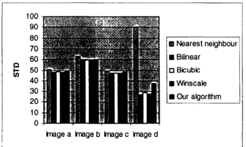
Figure 7: Standard deviation (STD) comparisons of the scaled down images.

In Figure 7, we use the standard deviation (STD) to compare the algorithms. Standard deviation can be used to give an estimate of the blur or contrast of an image; a high value generally means an image with few blur while a small value indicates a blurred image. The four images used for comparison are those of Figure 5. It appears that our algorithm gives good values of the standard deviation compared to the bilinear, bicubic or winscale algorithms. Only the nearest neighbour has higher values, and this was predictable since the nearest neighbour has very good contrast response although it degrades image quality due to aliasing. Thus, our algorithm seems to better reduce blur in comparison with the bilinear, bicubic and winscale algorithms.

Quantitative measures are generally not sufficient to compare various scaling algorithms. Qualitative comparison is also necessary although it is subjective and dependent on human

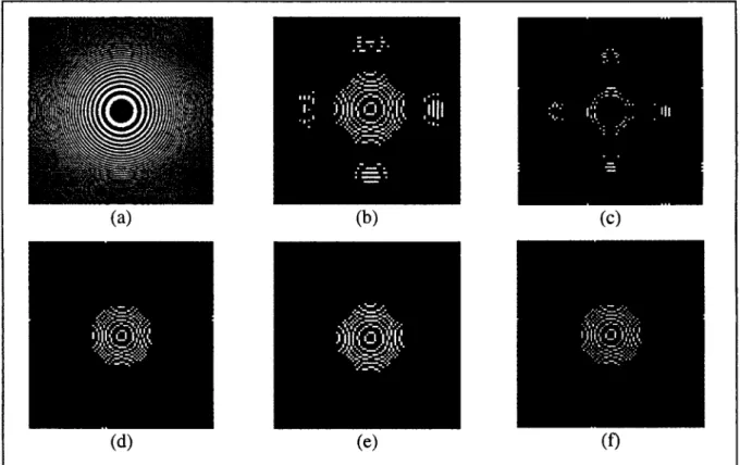
vision. Our algorithm has good edge characteristics. To see fine-edge characteristics, the edge maps of the scaled down images (with scale factor of 5/2) are shown in Figure 8; Sobel's filter was used to generate the edge maps. We have used the circular zone plate image (d) which has horizontal frequencies that increase as we move horizontally, and vertical frequencies that increase as we move vertically. As is shown in Figure 8, our algorithm better keeps the high horizontal and vertical frequencies than the other algorithms. The other algorithms lose more frequencies.

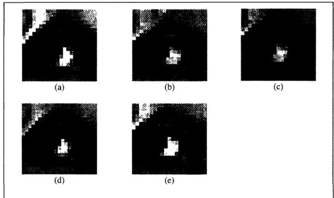
In Figure 9, we compare the aliasing generated by the different algorithms. The image of Lena is used in this step and we present the aliasing around the right eye of Lena. Our algorithm produces few aliasing compared to the nearest neighbour, bilinear and winscale algorithms. It appears to be comparable to the bicubic interpolation which also results in few aliasing.

Figure 8: The circular zoneplate image scaled down and edge map. (a) Original image (b) Our algorithm (c) Nearest neighbour (d) Bilinear interpolation (e) Bicubic interpolation (f) Winscale.

Figure 9: Aliasing on the right eye after scaling up by 5/2. (a) Our algorithm (b) Nearest neighbour (c) Bilinear interpolation (d) Bicubic interpolation (e) Winscale.

6 Conclusion

In this paper we have proposed a new and simple image scaling algorithm based on an area pixel model rather than the classic point-pixel model. A clear mathematical model has been described for the areas-pixels in the scaling process. We have compared our algorithm with some of the most popular scaling algorithms (nearest neighbour, bilinear and bicubic), and the tests have shown that our algorithm gives images of good quality with few aliasing, high contrast and few blur. It is better than the nearest neighbour and the bilinear algorithms concerning aliasing and compares well to the bicubic algorithm. It also has produces images with good contrast, few blur and good high-frequency response. Our algorithm also gives images of better quality compared to winscale, a previous constant areas-pixels-based resizing algorithm. For the future, more complex functions (wavelets, high order polynomials, etc.) can be used for describing the areas-pixels of an image. This may be

helpful for better details preservation and fewer blur and aliasing, but possibly at the expense of greater runtime.

7 References

[1] Andrews, S., Harris, F.: Polynomial approximations of interpolants. Conf. Record 33rd Asilomar Conf. Signals, Systems, and Computers 1:447-451 (1999)

[2] Battiato, S., Gallo, G., Stanco, F.: A locally-adaptive zooming algorithm for digital images, Elsevier Image Vision and Computing Journal 20(11):805-812 (2002)

[3] Carrato, S., Tenze, L.: A high quality 2x image interpolator. IEEE Signal Processing Lett, 7:132-134 (2000)

[4] Chan, R. H., Chan, T. F., Shen, L., Shen, Z.: Wavelet algorithms for high-resolution image reconstruction, Society for Industrial and Applied Mathematics, 24:1408-1432 (2003)

[5] Fifman, S.: Digital rectification of ERTS multispectral imagery. Proc. Significant Results Obtained From Earth Resources Technology Satellite-1. 1:1131-1142 (1973) [6] Gonzalez, R. C , Woods, R. E. (ed.): Digital Image Processing. Reading, MA:

Addison-Wesley (2002)

[7] Hore, A., Ziou, D., Deschenes, F.: A new image scaling algorithm based on the sampling theorem of Papoulis, Proceedings of the International Conference on Image Analysis and Recognition, Springer LNCS, 4633:1-11 (2007)

[8] Hou, H. S., Andrews, H. C : Cubic splines for image interpolation and digital filtering. IEEE Trans. Acoust., Speech, Signal Processing ASSP-26:508-517 (1978)

[9] Jain, A. K. (ed.): Fundamentals of Digital Image Processing, Englewood Cliffs, NJ: Prentice-Hall (1989)

[10] Kim, C. H., Seong, S. M., Lee, J. A., Kim, L. S.: Winscale: An Image-Scaling Algorithm Using an Area Pixel Model. IEEE Transactions on circuits and systems for video technology 13(6):549-553 (2003)

[11] Kim, H. C , Kwon, B. H., Choi, M. R.: An image interpolator with image improvement for LCD controller. IEEE Transactions on Consumer Electronics 47:263-271 (2001)

[12] Molina, R., Vega, M., Abad, J., Katsaggelos, A.K.: Parameter estimation in bayesian high-resolution image reconstruction with multisensors, IEEE Transactions on Image Processing, 12:1655-1667 (2003)

[13] Morales-Manilla, L., Sanchez-Diaz,G., Soto, R.: An image resizing algorithm for binary maps, Proceedings of the Fifth Mexican International Conference in Computer Science, 20(24): 126-132 (2004)

[14] Mukherjee J., Mitra. S. K.: Arbitrary resizing of images in DCT space, IEE Proceedings Vision, Image, and Signal Processing., 152(2): 155-164 ( 2005)

[15] Parker, J. A., Kenyon, R. V., Troxel D. E.: Comparison of interpolation methods for image resampling, IEEE Transactions on Medical Imaging 2:31-39 (1983)

[16] Pratt, W. K. (ed.): Digital Image Processing - PIKS Inside. New York: Wiley-Interscience (2001)

[17] Shezaf, N., Abramov-Segal, H., Sutskover, I., Bar-Sella, R.: Adaptive low complexity algorithm for image zooming at fractional scaling ratio. In 21st IEEE Conv. Electrical

and Electronic Engineers, Tel Aviv, Israel, pp. 253-256 (2000)

[18] Xiao, J., Zou X., Liu, Z., Guo, X.: Adaptive interpolation algorithm for real-time image resizing, First International Conference on Innovative Computing, Information and Control, 2:221-224 (2006)

[19] Ziou, D., Allili,M.: Image model: new perspective for image processing and computer vision, Proceedings of SPffi, Computational Imaging II, 5299:123-133 (2004)

Chapitre 2

Redimensionnement des images par le theoreme de

Papoulis

Dans ce chapitre, nous introduisons un algorithme de redimensionnement des images qui permet d'augmenter ou de reduire la resolution d'une image avec prise en charge des hautes frequences. En effet, les details d'une image, qui permettent de distinguer les objets et les formes, sont contenus dans les hautes frequences et doivent etre preserves autant que possible afin de ne pas perdre des informations importantes dans une image. La principale contribution de ce chapitre consiste a utiliser les derivees d'une image dans le processus de redimensionnement. Cette approche est motive'e par le fait que les derivees d'une image contiennent les informations sur les variations d'intensite de couleur des pixels, et done sur les hautes frequences. Afin de combiner, durant 1'interpolation, l'image originale et ses derivees, nous defmissons un modele de reconstruction d'images basee sur le theoreme d'echantillonnage generalise de Papoulis [12]. Ainsi, une image redimensionnee est vue dans notre modele comme la somme d'une image de basses frequences et d'une ou plusieurs images de hautes frequences. Soulignons ici que dans le precedent chapitre, le redimensionnement utilise essentiellement les techniques du calcul integral pour le calcul des moyennes de niveaux de gris, ce qui peut etre vu comme des filtres de basses frequences. Aussi, contrairement au chapitre precedent, nous considerons dans ce chapitre le pixel comme un point et non comme une unite surfacique. En effet, le theoreme de Papoulis utilise des echantillons discrets d'un signal pour reconstruire le signal continu.

Nous presentons, dans les pages qui suivent, un article intitule A New Image Scaling

Algorithm Based on the Sampling Theorem of Papoulis qui est paru dans les actes de

International Conference on Image Analysis and Recognition (ICIAR), Montreal, Canada,

2007 [29]. Le probleme a ete pose par le professeur Djemel Ziou. J'ai realise, valide et redige ce travail sous sa supervision. Le professeur Francois Deschenes a apporte de nombreux commentaires sur ce travail.

A New Image Scaling Algorithm Based on the

Sampling Theorem of Papoulis

Alain Hore, Djemel Ziou, and Frangois Deschenes

August, 2007

Abstract. We present in this paper a new image scaling algorithm which is based on the generalized sampling theorem of Papoulis. The main idea consists in using the first and second derivatives of an image in the scaling process. The derivatives contain information about edges and discontinuities that should be preserved during resizing. The sampling theorem of Papoulis is used to combine this information. We compare our algorithm with eight of the most common scaling algorithms and two measures of quality are used: the standard deviation for evaluation of the blur, and the curvature for evaluation of the aliasing. The results presented here show that our algorithm gives the best images with very few aliasing, good contrast, good edge preserving and few blur.

Keywords: Papoulis, image, resizing, scaling, curvature, derivatives, resolution.

1 Introduction

Image scaling algorithms are widely used in many applications going from simple personal pictures processing to complex microscopic defects identification. Scaling is desired because the resolutions of image sources are various and depend on their acquisition device, while the physical screen resolution of a digital display device is fixed [7]. Consequently, in the case where the resolution of an image is different from the screen resolution of a digital display device, we need to perform resizing. In the image-scaling process, image quality

should be preserved as much as possible; thus, we need to preserve edges and have few blur and aliasing.

The basic concept of image scaling is to resample a two-dimensional function on a new sampling grid [13, 14]. During the last years, many algorithms for image resizing have been proposed. The simplest method is the nearest neighbour [4], which samples the nearest pixel from original image. It has good high frequency response, but degrades image quality due to aliasing. The widely used methods are the bilinear and bicubic algorithm [5, 6]. Their weakness is blur effect causing bad high frequency response. Other complex algorithms have been proposed in the last years. Among them are the Lanczos algorithm, the Hanning algorithm and the Hermite algorithm [10]. They are mainly based on interpolation through finite sinusoidal filters. These algorithms produce images of various qualities which are generally better when the filter used has a shape close to the sine function. A new algorithm called winscale has been proposed [8] where pixels are considered as areas of constant intensity. This algorithm gives images with quality comparable to the bilinear algorithm. Other algorithms using adaptive [2, 15], correlative [9], polynomial [1] or fixed scale factors [3] properties have also been proposed in the last years. However, these methods are based on various assumptions (smoothness, regularity, etc.) which may lead to bad results when they are not satisfied.

In this paper, we introduce a new image scaling algorithm which is based on the generalized sampling theorem of Papoulis [12]. In signal processing, this theorem is used for perfect reconstruction of a signal given a set of its sampled signals. In our scaling algorithm, we take advantage of the information provided by the derivatives of an image in the resizing process. For example, the first derivative gives information about edges or regions of grey levels variations; also, the second derivative extracts image details more accurately. Combining this information (with Papoulis' theorem) during the resizing process tends to produce images of better quality than algorithms based on only the original image.

The outline of the paper is organized as follows: in section 2, we present the problem statement. In section 3, we describe the generalized sampling theorem of Papoulis. In section

4, we apply the theorem to image scaling. Section 5 presents the experimental results. We end the paper with the concluding remarks.

2 Problem Statement

The basic concept of image scaling is to resample a two-dimensional function on a new sampling grid. According to signal processing, the problem is to correctly compute signal values at arbitrary continuous times from a set of discrete-time samples of the signal amplitude. In other words, we must be able to interpolate the signal between samples. When we assume that the original signal is bandlimited to half the sampling rate (Nyquist criterion), the sampling theorem of Shannon states that the signal can be exactly and uniquely reconstructed for all time from its samples by bandlimited interpolation using an ideal low-pass filter. When the Nyquist criterion is not satisfied, the frequencies overlap; that is, frequencies above half the sampling rate will be reconstructed as, and appear as, frequencies below half the sampling rate [11]. This causes aliasing. In the case of image scaling, the effect is quite noticeable and leads to a loss of details of the original image. Several methods have been proposed in the last years to approximate the perfect reconstruction model of Shannon. They are generally based on finite interpolation filters with various analytical expressions ranging from polynomial to sinusoidal functions [10]. When the filter is very different from an ideal filter (sine function), aliasing and blurring occur [16]. Generally, the scaling algorithms are subject to the trade-off between high contrast, few aliasing and unnoticeable blur. This appears because the same finite filter is applied to both the low and high frequency components. Thus, in some cases the unique filter will tend to blur the image while in other cases aliasing will occur. To reduce the aliasing and blur effects, we propose to use image derivatives in the reconstruction process. The image derivatives enhance the high-frequencies. Blurring is attenuated because the use of enhanced high-frequencies enables a good preservation of contrast in the scaling process and prevents the image from being uniformly smooth. Aliasing is reduced because high-frequencies allow us to enhance both spatial and radiometric resolutions. To combine together the image and its partial derivatives, we propose to use the generalized sampling theorem of Papoulis [12]. This theorem enables

us, in the reconstruction process, to use the information provided by the derivatives of an image so as to better handle aliasing and blurring artefacts. In the next section, we present the generalized sampling theorem of Papoulis.

3 Papoulis' Sampling Theorem

Given a a-bandlimited function f{t) satisfying the following conditions: - / h a s a finite energy :

(2)

\\fitfdt

- / h a s a Fourier transform that vanishes outside the interval [-a, a].

The sampling theorem of Papoulis [12] gives an expression of J{t) as function of its sampling

gkinT) (k=l,...,m , n=-oo,...,oo) where the gk(t) are sampled at a low resolution T=mTo=nm/a (To=7t/o is the period of the signal/).

Given m linear systems H\(w),...,Hm(w), we pass through them the signaler) which is

a-bandlimited. Then, we obtain the following function gk(t):

1 a (3)

where F(w) denotes the Fourier transform of the signal/(r).

Papoulis' generalized sampling theorem states that the original signal f(t) can be reconstructed using the formula:

/(') = ! I s

(»r)*('-«r)

H](w)Y](w,t)+...+Hm(w,t)Ym{W,t)=\

(7)

Hl(w+rc)Yl(w,t)+...+Hm(w+rc)Ym(w,t)=e--Jrct

Hl(w+(m-\)c)Yl(w,t)+...+Hm(w+{m-[)c)Ym{w,t)=ej{

4 Using Papoulis' Sampling Theorem for Image Scaling

Let's define the following filters functions H\{w),...,Hm{w) in the Fourier domain:

"kMHJw?'

' *=l.".,m

In accordance with expression (2), Fourier transform properties give:

<\ ,(M/ \ , ,

**(')=/ '{t), k=l m

Thus, the signal/(0 can be expressed in function of its m-\ derivatives sampled at 1/m the Nyquist rate. In our model, we consider only the case where m=3 (we use the original image and its first and second derivatives), but we could choose any value. For m=3, we have

T=3iz/a and c=2a/3

Solving (4) and (6) yields:

3(l8+crV)sinV/3) °0 ) y.(0=

^ ( 0

Finally, using (3) we obtain:

/ ( f ) = 3 sin (<rt/3) I ( - i f n=-°° f(»T) -+-9 +f'(nT)- +r{nT)~-~ a(at-3nn) 2a (at-Inn) (11)

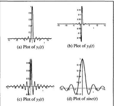
Figure 1 presents the different filters functions which are applied to the original signal and its derivatives. The plot of y\(t) shows that the filter has a high energy around the central point.

Even if some oscillations are noticeable, they are very damped in comparison to a sine function, and the filter function tends rapidly towards 0.

(a)Plotof;y,(0 (b)Plotof>2(r)

Figure 1: Plot of the filters functions.

Concerning the plot of the filter ^(O of the first derivative, we observe that it tends very rapidly towards 0 and the different contributions of the points around the central point are not high (less than 0.05). Thus, the influence of the first derivative seems to be smaller than that of the original signal during the resizing process. For calculation purposes, it is reasonable to consider a window of small half-width (5 for example) since the energy of the filter is concentrated in a small interval around 0.

The third plot in Figure 1 represents the filter function yi(t) applied to the second derivative. Here also, the contribution of the different points is very small (~ 10"3) compared to those of

the original signal and the first derivative. Thus, the influence of the second derivative is smaller than the original signal and the first derivative. The oscillations tends rapidly towards 0 but not as quickly as

y2(0-From Figure 1, it appears that our scaling algorithm may produce ringing effects due to the oscillations observed in the plot of the filters functions; however, they are quite unnoticeable because, unlike the sine filter, the contributions of the points causing these oscillations are not

significant to alter the rendered signal. Also, we observe that a small window can be considered for practical purposes since the filters have their energy mainly concentrated in small intervals around the central point.

5 Experimental Results

For implementation of the algorithm, we have T=\ and (T=3K. Also, we note that we have only considered ID signal in the previous section. In order to apply the algorithm to images, we use separability, that is we first compute only the columns of the image by using (10), and then we compute only the lines using the same formula. We also use a finite summation of (10). We have seen in the previous section that a small window could be used for the filters functions due to the concentration of their energies in small intervals around the central point. Generally, a window of half-width 5 gives good results (very few aliasing and blur) and there is no significant difference with windows of higher width.

Given a pixel located at (i,j), we use the following vertical derivatives (corresponding to lines):

[ lr n ( 1 2 )

jVJhfAiJh£f(i+W)-f(i-lJ)]

fVJ)=f~(iJ)=\[f(i+2Jh2f(iJ)+f(i-2j)]

The different steps of the scaling algorithms are as follows:

- Compute the first and second horizontal derivatives of the original image. - Use (10) to scale the image in the horizontal direction. This yields an image g. - Compute the first and second vertical derivatives of the image g.

- Use (10) to scale g in the vertical direction. This yields the original image scaled in the

horizontal and vertical directions.

The horizontal derivatives are computed in a similar way. The computational complexity of our algorithm depends on the size MxN of the original image, the scale factor R, and the width Wof the convolution filters y\, y2 and y*. The computation of the derivatives is O(MN) and the computation of the sum in (10) is 0(W2R2MN). Thus, the global computational

complexity of our algorithm is equivalent to that of the usual scaling algorithms based on convolution filters (for example, the algorithms of Lanczos and Hanning).

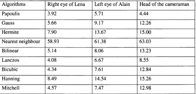
We have compared our algorithm to eight of the most popular resizing algorithms (nearest neighbour, bilinear algorithm, bicubic, Hermite, Mitchell, Hanning, Gauss and Lanczos interpolation). These algorithms are mainly based on polynomial or sinusoidal interpolation. Three images are used for the comparison between the different algorithms: "Lena", "Alain" and the "cameraman". The images are shown in Figure 2. For the experiments, the images are scaled up by a factor of 2, 4 and 8. For displaying purposes, the resized images have been adjusted to fit the page limits.

Figure 2: Images used in the experiments.

In Figure 3, we notice that the right eye of "Lena" is better observed in our model. The algorithms of Gauss and Mitchell produce noticeable blur. Images obtained using the Hanning algorithm, nearest neighbour or Hermite interpolation contain a lot of aliasing. The bicubic interpolation introduces little aliasing and the Lanczos algorithm yields a slightly blurred image.

Figure 4 illustrates the result for the left eye and cheek of the "Alain" image after resizing using our algorithm and the others presented previously for comparison. It clearly appears that our method gives the best results. There is fine contrast, less blur and unnoticeable aliasing while images obtained through Gauss and Mitchell algorithms produce visible blur. Images generated by Hermite, Hanning or bilinear interpolation are very aliased, and it is also the case for the nearest neighbour algorithm. Bicubic interpolation is slightly blurred but of good quality. The Lanczos algorithm also produces an image of good quality with few blur and aliasing.

Figure 3: Right eye of "Lena" after 2x scaling up.

In Figure 5, we show the result for the head of the "cameraman" using our algorithm and the eight other scaling algorithms. Here also, it is noticeable that our method gives the best results. There is less blur and few aliasing while images obtained through Gauss and Mitchell algorithms produce visible blur. Images generated by the nearest neighbour, Hermite, Hanning and bilinear interpolation are aliased. The Lanczos algorithm produces images of good quality comparable to our algorithm but with slight additional blur. Bicubic interpolation generates blur.

Table 1 presents the results of the computation of the standard deviation on some parts of the different images used for experiments: the right eye of "Lena" which is shown in Figure 3, the left eye and cheek of "Alain" which are shown in Figure 4 and the head of the "cameraman" which is shown in Figure 5. Standard deviation is a measure of the distance between pixels grey levels and their mean value. It's a dispersion criterion which can be used for estimating how blurred an image is: the more it has a high value, the less the image is blurred.

(a) Our algorithm

(g) Hanning

(b) Gauss (c) Bilinear

(h) Nearest neighbour (i) Lanczos

(g) Hanning (h) Nearest neighbour