Statistical Analysis of the time to publish clinical trial results

HAL Id: dumas-01059652

https://dumas.ccsd.cnrs.fr/dumas-01059652

HAL is a multi-disciplinary open access

archive for the deposit and dissemination of sci-entific research documents, whether they are pub-lished or not. The documents may come from teaching and research institutions in France or abroad, or from public or private research centers.

L’archive ouverte pluridisciplinaire HAL, est destinée au dépôt et à la diffusion de documents scientifiques de niveau recherche, publiés ou non, émanant des établissements d’enseignement et de recherche français ou étrangers, des laboratoires publics ou privés.

results

Rachel Heyard

To cite this version:

Rachel Heyard. Statistical Analysis of the time to publish clinical trial results. Methodology [stat.ME]. 2014. �dumas-01059652�

HEYARD Rachel

rachel.heyard@etu.unistra.fr

Université de Strasbourg

UFR de Mathématiques et d’Informatique

Master 1 Biostatistique

August 25, 2014

Statistical analysis

of the time to

publish clinical trial

results

Résumé

Dans ce rapport, on se consacre à l’analyse statistique d’un jeu de données constitué d’informations sur des essais cliniques sur les 53 nouveaux médicaments qui ont été approuvés par l’ « European Medical Agency » (EMA) entre 2009 et 2011. Ces données seront utilisées afin d’appliquer les utiles de l’analyse de la survie sur deux durées spécifiques. La première durée représente le temps entre l’achèvement d’une étude clinique et la publication des résultats qui en découlent. La seconde durée se définie comme la période entre la date où le médicament lié à l’essai clinique a été approuvé pour une première fois, soit par l’EMA, soit par la FDA (« Food and Drug Agency »), et la date de publication des résultats de l’étude clinique.

Après avoir expliqué le motif et les buts du projet dans le chapitre 1, le chapitre 2 s’intéresse à la théorie de l’analyse de survie. Par la suite, le chapitre 3 parle plus spécialement de la description de la base de données et de la résolution des problèmes rencontrés lors de l’importation des données dans le logiciel statistique R.

Le chapitre 4 a pour but l’illustration des résultats de l’analyse de survie sur les données. On commence par l’analyse de survie et la recherche d’un modèle de Cox pour la durée entre l’achèvement et la publication et on termine par l’analyse de survie et la recherche d’un modèle de Cox pour la durée entre l’autorisation de vendre un médicament particulier sur le marché et la publication des résultats d’essais cliniques liés à ce même médicament.

Finalement, le chapitre 5 tente de discuter les résultats, de tirer des conclusions et de vérifier les conditions d’applications des méthodes avant de passer à la bibliographie.

Remerciements

A cette occasion je voulais remercier mon maître de stage Pr. Stephen Senn pour m’avoir acceptée comme stagiaire et pour m’avoir offert la possibilité d’enrichir mes connaissances en statistique au sein de son centre.

Ensuite, je remercie aussi toute l’équipe du CCMS et du CES du CRP-Santé pour leur accueil chaleureux. Furthermore I would like to thank Bina Rawal and Bryan Dean for giving me access to their data and for their structural comments.

Table of Contents

Host Organisation ... 3

CRP-Santé ... 3

CCMS ... 3

Chapter 1: Introduction and objectives... 4

Chapter 2: Survival analysis ... 6

2.1.: General idea of the survival analysis ... 6

2.2.: The Kaplan-Meier estimator ... 8

2.3.: The log-rank test ... 9

2.4.: The cox proportional hazards model ... 10

2.5.: A package for survival analysis in R ... 10

Chapter 3: Data description and Handling ... 12

Chapter 4: Main results ... 17

4.1.: FIRST STUDY: Trial completion to publication ... 17

4.1.1.: Survival functions ... 17

4.1.2.: Comparison by covariates ... 19

4.1.3.: Cox regression ... 24

4.2.: SECOND STUDY: Regularity approval to publication ... 28

4.2.1.: Survival functions ... 28

4.2.2.: Comparison by covariates ... 30

4.2.3.: Cox regression ... 36

Chapter 5: Discussion and conclusion ... 38

Bibliography ... 40

Annexe I ... 41

H

OST

O

RGANISATION

CRP-Santé

The “Centre de Recherche Publique de la Santé” is located in Strassen, Luxembourg and was founded in 1988. Its main mission is to provide scientific, economic and societal knowledge by pursuing studies in biomedical research and public health. The research activities of the CRP-Santé are mainly conducted in the following five thematic research departments: Cardiovascular diseases, immunology, infection and immunity, oncology and public health.

For further information one can visit the website of the public research centre for health:

http://www.crp-sante.lu/.

CCMS

The “Competence Centre for Methodology and Statistics” (CCMS) was founded in March 2010 to satisfy the statistical needs of the other research centres of the CRP-Santé in Luxembourg. The activities of the competence centre include statistical support for project managers, developing statistical methodology of practical relevance to healthcare research, collaboration with external scientists working in fields of mutual interest and far more.

Head of the CCMS and supervisor of my traineeship that lasted 13 weeks is Prof. Stephen Senn. He is former Professor of Statistics at the University of Glasgow and former Professor of Pharmaceutical and Health Statistics at University College London. Moreover he worked as a statistician with the National Health Service in England and within the Swiss pharmaceutical industry.

C

HAPTER

1:

I

NTRODUCTION AND

O

BJECTIVES

There is now a common awareness of the importance of making clinical trial results publicly available. A failure in transparency in this domain conflicts with ethical duty towards patients which are involved in those clinical trials. Furthermore researchers should have at their disposal all available information before they take up further studies so that they prevent avoidable risks for patients.

One of the reason for this failure in transparency has been made out in an important number of studies as being the tendency of researchers and editors to prefer reporting positive trial results rather than negative trial results [1_,2_{]. In general reporting bias refers to a leaning to under-report depending on}

diverse characteristics of clinical trials, like the nature and direction of the results or the language of the publication.

In an interesting paper, Bina Rawal and Bryan Dean (R&D) [3_{] identified the proportion of clinical trials}

for which the results have been published within 12 months or by the end of the survey. In order to do this R&D searched the main clinical trial information sources for all sort of information on clinical trials related to the 53 new medicines approved by the European Medical Agency (EMA) in 2009, 2010 and 2011. Their main result was that 77% of the trials had results disclosed within 12 months of either the first regularity approval or the trial completion. This proportion had increased to 89% by the end of the survey period.

53 Excel spreadsheets – one for each medicine – have been sent to the CRP-Santé for further study. In this MSc project a survival analysis approach was used on the data from R&D in order to analyse the time to publish clinical trial results. During a first study of the data, it turned out that it would be best if two different survival analyses were made: One, analysing the time from trial completion to publication of trial results, and another, analysing the time between the first approval of the medicine by either the EMA or the Food and Drug Agency (FDA) and the publication of the trial results.

The US Food and Drug Agency Amendment Act (FDAAA) of 2007 says that it is compulsory for clinical trials’ summarized results to be posted on clinicaltrials.gov within one year of the study completion date. So, this MSc project tries to find out which proportion of clinical trials has failed to fulfil the requirements of the FDAAA.

1 _{Song, F., et al., (2009). BMC Med Res Methodol, p.79} 2 _{Senn, S., (2013). F1000Research, 1:59}

Then this project has as well the purpose to answer the question of which factors predict those times. Possible factors that might be associated with the time to publication are the study phase, the year of approval by the EMA as well as the size of the clinical trial. To know if these parameters are relevant for the time to public disclosure, Cox proportional hazard models were used.

C

HAPTER

2:

S

URVIVAL ANALYSIS

2.1.: General idea of the survival analysis

Survival analysis or analysis of lifetime deals with the study of a duration between a precise origin and the occurrence of an event. Usually this event is death, hence the name of this branch of statistics. The analysis of lifetime considers the evolution over time of the risk to die, it tries to find out what proportion of a population will still be alive after a certain time. This proportion is also called the population “at risk” to die.

T

:

Let X be the time until the event takes place.

 Cumulative distribution function: 𝐹(𝑡) = ℙ(𝑋 ≤ 𝑡)

It is the probability that the event takes place on or before time t.  Survival function: 𝑆(𝑡) = 1 − 𝐹(𝑡) = ℙ(𝑋 > 𝑡)

It is the probability that the event occurs after time t.

 Hazard function: 𝜆(𝑡) = lim

ℎ→0+

1

ℎℙ(𝑡 ≤ 𝑋 < 𝑡 + ℎ | 𝑋 ≥ 𝑡)

It is not really a probability but one can think of it as being the probability that the event occurs in an infinitesimally small period between t and t+1 given that the event did not occur before time t.

C

:

The survival time is often collected in an incomplete manner. An observation is called “censored” if the exact time until the event is unknown. For this observation we only have a partial information. For instance, when we know that the exact time is greater than a given value 𝑐 the observation is “right-censored”. If we know that the exact time is smaller than 𝑐 the observation is “left-“right-censored”.

Figure 1: time until event. Right-censored data.

In this illustration the three green lines represent right-censored observations. The first observation is for example right censored because this particular patient was alive during the whole study period. So, we only know that the lifetime of this patient is greater than the duration of the study. The second observation is right-censored because this subject has been lost to follow up before the event occurred. For the other three observations in blue we know the exact time until the event occurs. If X is the exact time until the event and if T is a censuring time we only observe the minimum of X and T.

2.2.: The Kaplan-Meier estimator

Definition: The Kaplan-Meier estimator is also known as the product limit estimator. It is commonly

used to estimate the survival function from lifetime data. More generally it is used to measure the length of the time until an event occurs. [In our study this estimator will measure the time until publication of results.]

Let 𝑇 be the length of time that an event needs to take place. The survival function 𝑆(𝑡) measures the probability that a certain individual requires a time greater than 𝑡 until the event takes place: 𝑆(𝑡) = ℙ(𝑇 > 𝑡).

If we have a sample of N observations, the observed times until the event of interest are: 𝑡1≤ 𝑡2≤ 𝑡3. . . ≤ 𝑡𝑁.

For each 𝑡𝑖, 𝑛𝑖 is the number of observations “at risk” shortly before 𝑡𝑖 and 𝑑𝑖 the number of events at 𝑡_𝑖. More precisely 𝑛𝑖 is the number of observations “at risk” at 𝑡𝑖−1 minus the number of events between 𝑡𝑖−1 and 𝑡𝑖 and minus the number of observations censored in this same time period. The maximum likelihood estimator of 𝑆(𝑡) is the Kaplan-Meier estimator 𝑆̂(𝑡):

𝑆̂(𝑡) = ∏ 𝑛𝑖−𝑑𝑖

𝑛𝑖

𝑡𝑖<𝑡 .

The Kaplan-Meier survival curve is graphically speaking a step function with a decline at each event time.

The estimated variance at time t is:

𝑉𝑎𝑟̂ (𝑆̂(𝑡)) = 𝑆̂(𝑡)2_∑ 𝑑𝑘

𝑛𝑘(𝑛𝑘−𝑑𝑘)

𝑘 ≤ 𝑡 .

Then, the confidence interval will be:

2.3.: The log-rank test

Definition: The log-rank test is a nonparametric hypothesis test that compares the survival distribution

of two or more samples. It is also called the Mantel-Cox test.

The test queries whether 𝐻0: no difference between survival curves, is verified or not.

In order to simplify the definition we only consider two sample groups, 1 and 2. Let 𝑑1𝑗 be the number of events in group 1 at time j and 𝑑2𝑗 be the number of events in group 2 at time j. Let 𝑛1𝑗 be the number of observations “at risk” in group 1 at time j and 𝑛2𝑗 be the number of observations “at risk” in group 2 at time j.

𝑑_𝑗= 𝑑_1𝑗+ 𝑑_2𝑗 ; 𝑛_𝑗= 𝑛_1𝑗+ 𝑛2𝑗

𝑑1𝑗 (as well as 𝑑2𝑗) has a hypergeometric distribution with as parameters ( 𝑛𝑗 , 𝑑𝑗 , 𝑛1𝑗 ). Then, 𝑈_𝐿= ∑𝑟 (𝑑_1𝑗− 𝑒_1𝑗) 𝑗=1 𝑤𝑖𝑡ℎ 𝑒1𝑗= 𝐸(𝑑1𝑗) = 𝑛_1𝑗 𝑑_𝑗 𝑛_𝑗 𝑉_𝐿= 𝑉𝑎𝑟(𝑈_𝐿) = ∑𝑟 𝑣_1𝑗 𝑗=1 𝑤𝑖𝑡ℎ 𝑣1𝑗= 𝑉𝑎𝑟(𝑑1𝑗) = 𝑛1𝑗 𝑛2𝑗 𝑑𝑗 (𝑛𝑗−𝑑𝑗) 𝑛_𝑗2 _(𝑛 𝑗− 1) → 𝑈𝐿 √𝑉𝐿 ~ Ɲ(0,1) 𝑊_𝐿 ≔ 𝑈𝐿 2 𝑉_𝐿 ~ 𝑥2(1)  𝐻₀ has to be rejected if 𝑊_𝐿≥ 𝑥_1−∝2 ₍₁₎

2.4.: The Cox proportional hazards model

Definition: The hazard function which calculates the instantaneous risk for the event to occur at time

t conditional on survival to that same time t is: ℎ(𝑡) = lim

𝛥𝑡→0

𝑃[(𝑡 ≤ 𝑇 < 𝑡 + 𝛥𝑡) ∣ 𝑇 ≥ 𝑡] 𝛥𝑡

where 𝑇 is the length of time that an event needs to take place.

Definition: Cox proportional hazards models are used to examine the relationship of a survival

distribution to covariates. This model was proposed by Cox in 1972.

Let 𝑥1, 𝑥2, … , 𝑥𝑚 be the 𝑚 covariates, 𝛽1, 𝛽2, … , 𝛽𝑚 be the 𝑚 coefficients and 𝛼(𝑡) = log(ℎ0(𝑡)) be the baseline hazard function.

The Cox model for the observation i is:

logℎ_𝑖(𝑡) = 𝛼(𝑡) + 𝛽₁𝑥_𝑖1+ 𝛽₂𝑥_𝑖2+. . . +𝛽_𝑙𝑥_𝑖𝑚 or equivalently,

ℎ_𝑖(𝑡) = ℎ₀(𝑡)exp(𝛽₁𝑥_𝑖1+ 𝛽₂𝑥_𝑖2+. . . +𝛽_𝑙𝑥_𝑖𝑚).

The hazard ratio for two observations i and i', _ℎℎ𝑖(𝑡)

𝑖′(𝑡)=

𝑒𝛽𝑋𝑖

𝑒𝛽𝑋𝑖′, is independent of the time t. Hence, the

2.5.: A package for survival analysis in R

To compute the survival analysis on the data the R package {survival} is used. This package has been written by Terry M. Therneau and ported to R by Thomas Lumley.

F

:

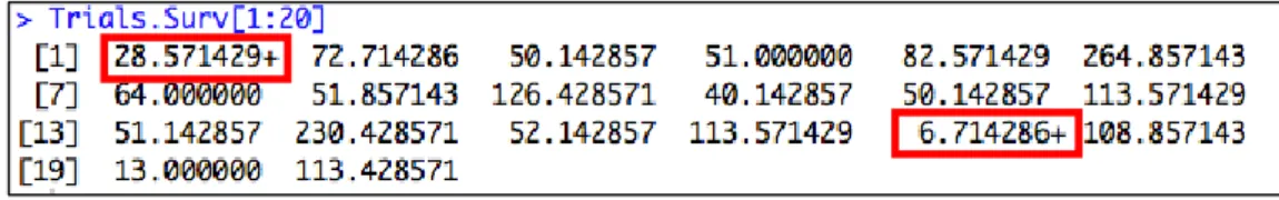
Surv( ): It is a so called ‘packaging function’ that creates a survival object. Furthermore, to transform

right censored data into a survival object Surv(time, status) is used, where time is the duration of interest and status an indicator of whether the observation is right censored or not. In R a survival object has the following appearance:

Figure 2: Survival object in R.

Censored observations are marked with a “+”. For instance, 28.571429+ means that the trial had no results published 28.57 weeks after his completion and was then unavailable. The results have not been published by the end of the study period.

Survfit( ): This function fits a survival curve – simple Kaplan-Meier (K-M) or several K-M curves split

by one or more covariates. The Kaplan-Meier estimator permits the calculation of an estimated survival function. It is a step function where each step means a decrease of (1 −_𝑛1

𝑡) of the estimated survival

if there is an event at time t and a number of 𝑛𝑡 trials are still unpublished.

…..

Figure 3: Summary of a survfit object in R. The panel displays for every event time

the value of the survival function as well as the number of events and the number of observations “at risk”.

Survdiff( ): Applied on a survfit object this function computes a log-rank test.

Coxph( ): This function, applied on a survfit object, creates a Cox proportional hazards model. Cox.zph( ): It computes a test of proportional hazards for a previously fitted Cox model.

C

HAPTER

3:

D

ATA DESCRIPTION AND

H

ANDLING

We have a dataset of 1007 completed clinical trials associated with medicines approved in 2009, 2010 and 2011 by the European Medicines Agency (EMA). During this 3 year period 53 new medicines were approved by the EMA. Rawal and Deane (R&D) collected the data on various publicly available information sources like http://www.clinicaltrials.gov during the study period, 27 December 2012 to 31 January 2013 inclusive.

53 Excel spreadsheets for every approved medicine were provided by B. Deane for further study. Only 52 medicines are retained because the medicine ‘Fridapse’ was approved on historical data and we received incomplete and not useful information for this particular medicine.

For every medicine we got all kinds of interesting data on the connected clinical trials like the phase in which the trial took place, the number of patients who participated in the trial, the trial completion date, the earliest date of posting summary results or the full publication date. Moreover, for all medicine the date of approval by the EMA as well as the date of approval by the Food and Drug Administration (FDA) – if the medicine has been approved in the US – was given.

In the interest of importing the data into the R software the format of all the dates was changed manually. As to the completion date, the Excel spreadsheets furnished sometimes a primary completion date and a study completion date. On www.clinicaltrials.gov I found the following definition of the two dates:

[Primary Completion Date: As specified in US Public Law 110-85, Title VIII, Section 801, with respect to an applicable clinical trial, the date that the final subject was examined or received an intervention for the purposes of final collection of data for the primary outcome, whether the clinical trial concluded according to the pre specified protocol or was terminated.

Study Completion Date: Final date on which data was (or is expected to be) collected.] [4]

R&D chose the study completion date in their analyses. If this study completion date is available R&D’s approach is used, else, for the sake of consistency, the trial completion date is left missing.

As for the publication date we took the earliest date of either posting of summary results or full publication. If no publication date has been given, the exact time to publication will not be observed.

To considerate these censored observations the publication date is set to 31 January 2013, the end of the study period and, in addition, a variable called status is added. It indicates by a value of 1 that the results of a certain clinical trial have been published by the end of the study period and by a value of 0 that the exact publication date is unknown. So, a status variable that equals zero indicates a right censored observation. Two publication dates are missing in the cohort because in the Excel spreadsheets received from R&D was indicated that those trial results have been published but the date is not given. Those two observations are excluded for the survival analysis.

A new variable called FirstApproval which contains the minimum of the dates of approval by the EMA and the FDA is created.

The variables used as time information for the survival analysis are time and time2 which represent the differences in weeks between two dates of interest. time is the number of weeks between the trial completion date and the publication date, time2 represents the number of weeks between the date of first approval and the publication date.

Concerning the study phase, since phase IV-studies are done after the drug has been put on the market we decided to exclude all phase IV trials as well as those classified as ‘other’ from the cohort. Then, because the frequency for phase I/II and for phase II/III is very low we decided to merge phase I/II with phase II and phase II/III with phase III.

Table 1: Features of the 1007 clinical trials:

Feature Number (percentage)

Phase Phase I 111 (11%) Phase II 401 (40%) Phase III 433 (43%) Phase IV 39 (4%) other 23 (2%)

Year of approval by the EMA 2009 521 (52%)

2010 223 (22%)

2011 263 (26%)

Median Mean Range Missing

Number of patients involved 163 480.5 1 – 18624 50

It is not shocking that the most important proportion of completed trials are linked to 2009 approvals. As R&D’s study period ended 31 January 2013 it appears that the results of some trails were not published by then. This does not mean that the results of those specific trials will never be published. It only means that the time to publish the results of those trials will be greater than the difference

between the completion date and the end date of the study period but we cannot know how much. This data is right-censored.

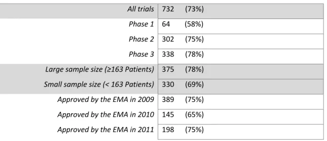
Table 2: Number of trials with published results by the end of the study period

All trials 732 (73%) Phase 1 64 (58%) Phase 2 302 (75%) Phase 3 338 (78%) Large sample size (≥163 Patients) 375 (78%) Small sample size (< 163 Patients) 330 (69%) Approved by the EMA in 2009 389 (75%) Approved by the EMA in 2010 145 (65%) Approved by the EMA in 2011 198 (75%)

I

Some dates – both, dates of completion and dates of publication – are incomplete. For an important proportion of dates the day of the month is missing. For consistency, we decided to take the 15th _{of the month.}

But there are also dates where even the month is missing; only the year of the trial completion respectively the publication of the results is furnished. To resolve this problem an R function has been written to simulate a random date between 1 January and 31 December of the particular year. [R code of the function to be found in Annexe II.]

In 2009 this issue occurred 30 times, in 2010 twice and in 2011 seven times.

In order to know if the fact of using a simulated date instead of the exact date has an impact on the results of our study three different datasets for 2009 are created where the respective dates are simulated independently. Afterwards three distinct Cox regressions try to explain the time between the completion of the trial and the publication of the related results by considering the phase of the trial.

Those three Cox regression models furnished different parameters for the hazard ratio between phase I and phase III:

Table 3: Test on hazard ratios Exp(Coef) = hazard ratio Confidence Interval

Dataset 1 1.475 [0.959 , 2.27]

Dataset 2 1.474 [0.959 , 2.27]

Dataset 3 1.471 [0.959 , 2.26]

The hazard ratios differ only very little as well as the confidence intervals for these hazard ratios. So, in conclusion, we can assume that the fact of using random dates for the survival analysis will have no effect on the results of a survival analysis.

P

Since we decided to only work on phase one to three trials, all the other observations are deleted form the cohort as well as the two observations with a missing publication date, leaving us with 943 leftovers.

Those observations with missing completion dates (165 of 943 clinical trials) are excluded for the first study, the one that takes the study completion date as origin. So, 778 trials are at the disposal for the first study.

For the second study, the one that takes the first date of approval as origin, 228 trials (24.18%) have their results published before the related medicine has been approved by the EMA or the FDA. To illustrate the Kaplan-Meier survival curves and to take into account this information we zeroed those 228 trials’ time2 variable. For this study I had 943 observations left.

V

“

”

The first study compares the study completion date to the earliest date of summary results posted on a registry or publication in the scientific literature.

We create the variable time which is the difference in weeks between the trial completion date and the results’ publication date. 45 time periods created by the difftime function in R are negative because first results of those trials were published before the data was collected completely. 45 trials represent 5.8% of all remaining trials. We suppose that most of those negative time values arise from

the fact that primary endpoint results have been published whereas the study completion date refers to a follow-up date a year or more after. Since a survival analysis has to be done using this variable time these trials cannot be used and have to be deleted from the cohort. We have 733 leftovers.

V

“

2”

The second study is a sort of conditional analysis. Here we compare the dates of first approval by either the EMA or the FDA and of publication of first results.

We create the variable time2 which is the difference in weeks between the two dates of interest. To do so, the R function difftime is used.

In order to take into account the fact that at time=0 24% of the trials have their results already published the time2 variable of those observations is set to zero in order to illustrate the survival curves. For the Cox regression those observations are excluded from the cohort. So, 943 trials are left for the survival curves and 682 trials are left for the Cox regression.

V

Drug – name of the medicine Year – year of approval by the EMA

Ph – phase of the trial, in (I, I/II, II, II/III, III, IV, other)

TotalPatients – total number of patients involved in the trial Cat – category a, b, c or d depending on the size of the trial D_of_completion – date of the trial completion

D_publication – date where the first result have been published

FirstApproval – date of the first approval by whether the EMA or the FDA Status – variable indicating whether the data is right-censored or not, in {0,1} Time – difference in weeks between d_of_completion and d_publication Time2 – difference in weeks between FirstApproval and d_publication

C

HAPTER

4:

M

AIN RESULTS

4.1.: FIRST STUDY: Trial completion to publication

4.1.1.: Survival functions

For this first survival analysis 733 trials are at our disposal. 542 trials – 74% – have achieved public disclosure of their results at the end of the study period. The remaining observations are right-censored.

The plot function applied on a survfit object allows a graphical representation of the Kaplan-Meier estimates.

Figure 4: Kaplan-Meier survival curve with all the data. The X axis indicates the number of

weeks from the study completion dates to the publication of results, the Y axis indicated the proportion of trials that did not achieve public disclosure of results.

Here, we have the proportion of trial results not published after a given number of weeks. So, after 200 weeks (approximately 3 years and 10 months) there are still about 20% of the trials which don't

see their results published. The sharpest decrease of the proportion of trials that are not published at a certain amount of weeks is to be found 52 weeks after the study completion. The markings on the curve indicate censoring time and the bands give the approximate confidence intervals.

The maximum of weeks that it takes to publish trial results is 1294 weeks. This large figure in weeks is due to the fact that this specific trial was terminated in 1988 and the results have not been published by 31 January 2013, the end of the study period.

In our study, a more clear representation would be the inverse survival function that is achieved by adding the option fun=‘‘event’’ to the plot of the survfit object.

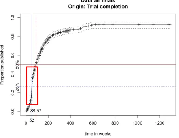
Figure 5: Inverse Kaplan-Meier survival curve with all the data. The X axis indicates the number

of weeks from the study completion dates to the publication of results, the Y axis indicates the proportion of trials that achieved public disclosure of results.

This graph shows the proportion of results published a certain amount of weeks after the study completion date. So, after 52 weeks 26% of all the trials related to medicine approved by the EMA in the three year period see their results published. 50% of the trial results are published 88.57 weeks (about 1 year an 8 months) after the trial completion. Again, the markings on the curve indicate censoring time and the bands give the approximate confidence intervals.

Moreover it seems that there is a lot of pressure to publish results within one year (52 weeks). The most important increase of the curve is visible shortly before and after 52 weeks → . This evolution is probably due the Food and Drug Administration Amendments Act (FDAAA) of 2007 which requires clinical trials to publish basic results to clinicaltrials.gov within one year of the study completion.

4.1.2.: Comparison by covariates

4.1.2.1: Split by year of approval by the EMA

So as to compare the survival functions for the three years three different survival functions are represented on the same plot, one for 2009, one for 2010 and one for 2011 approved medicines by the EMA.

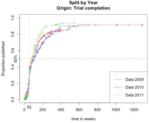
Figure 6: Inverse Kaplan-Meier survival curve split by year of approval by the EMA. Completion to publication.

We are in the presence of more or less the same curves until one year has passed after the study completion. Then trials for 2011 approved medicines have their results posted faster than 2010 and 2009 approvals.

To test whether the three survival curves split by year are identical or not I computed a log-rank test with the survdiff function in R.

Table 4:

Median weeks from

completion to publication p-value of the log-rank test Approved by the EMA in 2009 89

0.0946 > 0.05

Approved by the EMA in 2010 109.5

Approved by the EMA in 2011 80.5

Since a p-value of 0.0946 is not significant we cannot conclude that the three curves are significantly different. On the contrary, we have to accept the assumption of identical survival curves. This test says that the effect of the variable Year on the time to publication cannot be significant.

4.1.2.2.: Split by study phase

Likewise, a comparison of the survival function split by study phase can be done so as to see if there is a phase-effect on the time to publish clinical trial results after the completion of the trial.

Figure 6: Inverse Kaplan-Meier survival curves split by study phase.

From the graph we can tell that phase III trials have their results posted the fastest. After only 148 weeks, 80% of the results of phase III trials have been posted. Phase II trials need 324 weeks to publish 80% of the trial results and phase I trials even need 544 weeks.

Table 5:

Median weeks from completion to publication

p-value of the log-rank test

Estimated hazard ratio (95% CI)

𝝀𝑷𝒉𝒂𝒔𝒆 𝒊 𝝀𝑷𝒉𝒂𝒔𝒆 𝟏 ⁄ 𝒘𝒊𝒕𝒉 𝒊 = 𝟐, 𝟑 Phase I trials 143 < 0.001 1 Phase II trials 108.7 1.36 (1 - 1.87)

Phase III trials 69.1 2.1 (1.54 - 2.87)

The median of the weeks that it takes from completion to publication decreases a lot from phase I to III trials. The results of the log-rank test applied to the survival function split by phase show that we have to reject the null hypothesis which says that the survival curves for the 3 different phases are identical. So, it seems that there is a phase-effect. To find out if there really is a phase-effect a Cox model with as single regressor the study phase is used. The R output furnished the different hazard ratios, the one between phase I and phase II and the one between phase I and II; R took phase I as a reference. The third hazard ratio in the table is highly significant so that we can affirm that phase III trials have their results publicly disclosed 2.1 times faster than phase I trials.

To verify the assumption of an effect of the study phase on the time from completion to publication we apply the anova function on the Cox model in R.

Table 6: ANOVA output LN(Maximum likelihood) p-value

Null model -3114.9

Cox model with covariate Phase -3096.8 <0.001

It compares the null model with the Cox model. The Akaike Information Criterion (AIC) will be smaller for the Cox model since AIC = 2k – 2ln(L) where k is the number of parameters and L the maximized value of the likelihood function. The model that presents the smallest AIC coefficient best describes the data.

Moreover, the deviance between the two models is significant given that the p-value is much smaller than 0.05. This is why we can conclude that there exists a phase-effect on the time from completion to publication because the Cox model with phase as covariate has a significantly smaller deviance than the null model.

4.1.2.3.: Split by trial size

A last comparison we can process is the comparison of the survival curves for different numbers of patients participating in a clinical trial. The trials for whom no information on the amount of patients is given are excluded for the following confrontation of survival curves. To do so a new variable called Cat that takes the values a, b, c and d depending on the number of patients in a trial is created. The quantiles for the number of patients involved in a trial helped to make out the limits of the different groups.

The category 'a' regroups the trials with the fewest patients and category 'd' the trials with the most patients involved.

Figure 7: Inverse Kaplan-Meier survival curves split by category. Completion to publication.

Table 7: Quantiles of the number of patients

0% 25% 50% 75% 100%

At first sight, the four inverse survival curves seem identical until 52 weeks have past. After this moment they differ more and more, though the survival functions for categories 'a' and 'b' and for categories 'c' an 'd' are very similar. After all, one can say that clinical trials which include more than 164 patients see their results published much faster than those implicating less patients.

Table 8:

Median weeks rom completion to publication

p-value of the log-rank test

Estimated hazard ratio (95% CI)

A: ≤164 77

<0.001 0.72 (0.61 – 0.86)

B: >164 99.7 1

The median of weeks between the trial completion and the publication of the trial results for the two groups differs a lot. In addition, since the p-value of the log-rank test is highly significant the assumption of identical survival curves has to be rejected. It appears that there could be an effect of the number of patients on the time from completion to publication.

To receive certainty about this effect of the category a Cox model with as single regressor an indicator on whether there are more or fewer than 164 patients involved in the trial is fitted. R took the trials with more than 164 patients as a reference. The estimated hazard-ratio of 0.72 says that trials with fewer patients involved need more time to achieve public disclosure of results. Moreover, this hazard-ratio is highly significant since 1 is not included in the confidence interval.

In order to know if there is an overall effect of the number of patients on the time from completion to publication we apply the anova function on the Cox model.

Table 9: ANOVA output LN(Maximum likelihood) p-value

Null model -3007.4

Cox model with covariate (Number of patients > 164) -3000.6 < 0.001

The AIC coefficient will be smaller for the Cox model with a covariate indicating whether more or fewer patients are involved in a trial than the AIC for the null model. In addition the deviance between the two models is statistically significant due to a p-value smaller than 0.05. This demonstrates the existence of an effect of the number of participants in a clinical trial on the time from study completion to publication of the results.

C

We discovered an effect of the phase and of the number of patients but no year-effect on the time from study completion to public disclosure of results. Now we will try to find the best Cox regression model so that we can estimate the number of weeks from completion to publication by considering different covariates.

4.1.3.: Cox regression

We begin with a naïve model including all 3 covariates, meaning the year of approval by the EMA, the phase of the trial and the logarithm of the number of patients involved in the clinical trial. The logarithm is used because the amount of patients is very widespread.

T

Figure 8: R output of summary function applied on Cox model. R took the phase I trials for

In order to know if there are effects on the time between trial completion and publication of results by the covariates the anova function is applied on the newly fitted Cox model:

Figure 9: R output of anova function applied on Cox model.

The null model has the highest AIC coefficient. So whatever covariate chosen for the Cox regression this model will always be better than the null model. The most significant covariate is ph which indicates the phase of a clinical trial. The covariate TotalPatients shows no significant p-value even though an effect by the number of patients involved in a trial on the time to publication was discovered previously so that it can be concluded that when the covariate ph is present in the model TotalPatients is not needed to describe the time until publication. This is probably due to the fact that the number of patients is explained by the phase of the trial and vice-versa.

The covariate Year, which indicates the year of approval of the medicine by the EMA, seems to have no significant effect.

A way to find the best covariates for the Cox model is to use the stepAIC function of the package {MASS}:

Figure 10: StepAIC function applied on Cox model.

The function starts with a Cox model with as covariates Year, ph and the logarithm of TotalPatients. This model has an AIC coefficient of 5976.5. By dropping the logarithm of

TotalPatients the AIC would decline to 5975. Since the model that minimizes the AIC is the model with the most quality R continues with the Cox model without the number of patients. By dropping the variable ph or Year the AIC would increase.

The best Cox model is thereby the one with a covariate indicating the phase of the trial and the year of approval of the related medicine by the European authorities.

The summary of this Cox model found by the stepAIC function is:

Figure 11: R output Summary function applied on Cox model. R took phase I trials for

medicines approved in 2009 by the EMA as a reference.

Time from completion to publication for results emerging from phase III trials is statistically significantly lower than the time to publish results of phase I trials, for 2009 approved medicine. Phase II trial results’ chance to be published is 1.35 times greater than phase I trial results’ chance for 2009 approved medicines. For 2009 approved medicines by the EMA, phase III trial results are even posted more than 2 times faster than phase I trials. For phase I trials, those approved in 2011 have a 1.19 greater chance of being published than those approved in 2009.

Is this model better than the null model?

Table 10: ANOVA output LN (Maximum likelihood ) p-value

Null model -3007.4

Cox model with covariate Year -3004.9 0.077

Cox model with covariate Phase -2983.5 < 0.001

The AIC for the null model is significantly higher than for the other models. By adding the covariate indicating in which year the medicine was approved by the EMA the AIC coefficient decreases but this decrease is not very significant. So, there is no significant effect of the year of approval by the EMA on the time from completion to publication.

In the contrary, we made out a huge effect of the study phase on the time to publication since the third p-value is highly significant.

4.2.: SECOND STUDY: Regularity approval to publication

4.2.1.: Survival functions

For this second study we have 943 trials at our disposal. The work is done on the variable time2, the difference in weeks between the date of first approval of the medicine by one of the authorities and the date of publication of the results of the related clinical trial. 702 trials – 74.4% – have achieved public disclosure of their results by 31 January 2013. The other 241 observations are right censored. Graphically the Kaplan-Meier survival function has the following shape:

Figure 12: Kaplan-Meier survival curve with all the data. The X axis indicates the number

of weeks from the regularity approval to the publication of results, the Y axis indicated the proportion of trials that did not achieve public disclosure of results.

The proportion of trial results not published starts at approximately 0.76 because at the moment of the approval of the medicine 24% of the trials have their results already published.

A more appropriate representation to illustrate our data would be the inverse survival curve which is done by adding the option fun=‘‘event’’ to the plot function.

Figure 12: Inverse Kaplan-Meier survival curve with all the data. The X axis indicates the number

of weeks from the regularity approval to the publication of results, the Y axis indicated the proportion of trials that did achieve public disclosure of results.

Here, we have the proportion of trials with results published a given number of weeks after the connected medicine has first been approved by either the EMA or the FDA. Unlike the first study, we don’t see proof that there is pressure to publish the results 52 weeks after the medicine has first been approved. But, almost 50% of the trials have their results posted one year after the related medicine has been approved by the authorities.

4.2.2.: Comparison by covariates

4.2.2.1.: Split by year of approval by the EMA

Firstly, we compare the survival curves split by the year of approval by the EMA.

Figure 13: Inverse Kaplan-Meier survival curves split by year of approval by the EMA. Regularity approval to publication.

Approximately 60% of the trials related to medicines approved in 2011 by the EMA have their results posted one year after the connected medicine has first been approved by one of the authorities. The other trial results are published less fast. The data for 2009 and for 2010 approved medicines have a similar distribution, the distribution of the data for 2011, on the other hand, diverges a lot.

Table 11:

Median weeks from regularity approval to publication

p-value of the log-rank test

Estimated hazard ratio (95% CI)

Approved in 2009 by the EMA 103

< 0.001

1

Approved in 2010 by the EMA 99.1 1.09 (0.89-1.33)

Approved in 2011 by the EMA 23.7 2.02 (1.68-2.44)

The median weeks from regularity approval to publication for 2009 and 2010 approved medicines by the EMA does not differ a lot. Furthermore, the estimated hazard ratio between 2009 and 2010 is not significantly different from 1. Elsewise, the median weeks is much smaller for 2011 approvals. The hazard-ratio between 2009 and 2011 is significantly different from 1 so that one can say that trials for 2011 approved medicines are publicly disclosed two times faster than those approved in 2009. It seems like there is an effect of the covariate Year on the time from approval to publication. So, these results differ from the one of the first study. The variable Year had no proven effect on the time between the trial completion and the publication of its results.

To verify this assumption of the existence of an effect by Year we apply the anova function on the newly fitted Cox model.

Table 12: ANOVA output LN (Maximum Likelihood) p-value

Null model -4322.1

Cox model with covariate Year -4294.9 <0.001

This table demonstrates that there is an effect by the year of EMA approval on the time from regularity approval to publication of the results because firstly the AIC for the Cox model is smaller than the one for the null model and, secondly, this difference is significant due to a p-value smaller than 0.05.

4.2.2.2.: Split by study phase

The survival curves split by the phase of the trial have the following appearance:

Figure 14: Inverse Kaplan-Meier survival curves split by study phase. Regularity

approval to publication

Phase III trial results seem to be published the fastest: 202 weeks – nearly 4 years – after the first approval by the EMA or the FDA, 80% of the results are published. The other trials, phase II and I, need a lot more time in order to have published 80% of the trial results.

Table 13:

Median weeks from regularity approval to publication

p-value of the log-rank test

Estimated hazard ratio (95% CI) Phase I 150.4 0.00337 1 Phase II 61.8 1.37 (1.05 – 1.80) Phase III 64 1.52 (1.17 – 1.99)

The median of weeks from approval to publication for phase I and II trials is nearly the same. Due to a significant p-value of the log-rank test we can reject the assumption of identical survival curves. Moreover, phase II trials’ chance to achieve public disclosure of their results is 1.37 times greater than phase I trials’ chance to publication. Phase III trials are even 1.52 times faster published than phase I trials. The two hazard ratios are statistically significant since their confident intervals do not include 1. The anova function applied on the Cox model with as covariate the study phase has the following results:

Table 14: ANOVA output LN (Maximum likelihood) p-value

Null model -4322.1

Cox model with covariate phase -4316.8 0.0053

This table puts out the fact that the time from regularity approval is influenced by the study phase because the AIC is significantly lower for the Cox model due to a significant p-value.

4.2.2.3.: Split by trial size

The last comparison is the one of the survival curves split by the category indicating the size of a trial. We deleted the observations where the information on the number of patients is missing, then we created the four categories by making use of the following quantiles.

Table 15: Quantiles of the number of patients involved

0% 25% 50% 75% 100%

2 43.5 162 423 18624

We have 899 remaining observations to do the survival functions.

Figure 15: Inverse Kaplan-Meier survival curves split by trial size. Regularity

approval to publication.

One year, 52 weeks, after the approval of the medicine by the authorities the most important proportion of trial results published has to be found in the category 'd', the biggest trials. Categories 'a' and 'b' have more or less the same distribution, so that I decided to merge them for the log-rank test.

Table 16:

Median weeks from regularity approval to publication p-value of the log-rank test Estimated hazard ratio (95%) Small trials: [2,162[ 95.3 < 0.001 1 Intermediate trials : [162,423[ 64.4 1.31 (1.09 – 1.58) Big trials: >423 29.3 1.72 (1.43 – 2.07)

The median of weeks from regularity approval to the publication of results decreases a lot from small to big trials. The p-value of the log-rank test is highly significant so that we have to reject the null hypothesis of identical survival curves. Furthermore the significant estimated hazard ratio between small and intermediate trials means that intermediate trials have a 1.31 times bigger risk of being published than small trials. The publication risk for big trials is 1.72 times bigger than the one for small trials.

By applying the anova function on the Cox-model with as covariate the three categories we get the following result:

Table 17: ANOVA output LN (Maximum likelihood) p-value

Null model -4130.1

Cox model with covariate size of trial -4113.5 < 0.001

Since the AIC coefficient is smaller for the Cox model with a covariate indicating the size of the trial and this deviance is significant we can conclude that there is an effect of the number of patients on the time from approval to completion.

C

Three effects on the time from regularity approval to public disclosure of results are made out by the second survival analysis. Now we will try to find the best Cox regression model so that the number of weeks from approval to publication can be deviated by considering the study phase, the year of approval of the related medicine by the EMA and the number of patients involved in the trial.

4.2.3.: Cox regression

A naïve Cox model would be a model containing the three possible covariates, Year, ph and TotalPatients. In order to have less parameters we use the number of patients in a continuous way instead of the categories. However we have to use the logarithm of the number of patients in a trial since this amount is very widespread.

T

C

:

Figure 16: R output summary function applied on naïve Cox model. R took phase I trials for

medicines approved in 2009 by the EMA as a reference.

A phase III trial related to medicine approved in 2009 has a 2.744 times bigger risk of achieving public disclosure than a phase I trial related to 2009 approved medicine. A phase I trial’s publication risk is 1.5 times bigger if the related medicine is approved in 2011 instead of in 2009.

In order to know if this Cox model is better than the null model we apply the anova function on the newly fitted Cox model:

Table 18: ANOVA output LN (Maximum likelihood ) p-value

Null model -2682.6

Cox model with covariate Year -2653.5 <0.001

Cox model with covariate Phase -2637.7 < 0.001

Cox model with covariate log(Total Patients) -2635 0.01928

So, the time until publication depends on the year of approval of the medicine, the phase of the trial and the number of patients involved.

After having applied the Cox model on the stepAIC function to find the covariates which best predict the number of weeks between the regularity approval and achievement of public disclosure we find out that the naïve Cox model is the one presenting the smallest AIC coefficient.

C

HAPTER

5:

D

ISCUSSION AND CONCLUSION

In order to summarize the results we can highlight the following conclusions:

First of all the time from study completion to result publication is particularly influenced by the study phase. So that if we are aware of the study phase we are capable of making assumptions on how long it will take the clinical trial to achieve public disclosure of its results. However there are other factors predictive of this time from completion to publication which could not be treated in this survival analysis. It has suggested in lots of studies that the nature of the outcome of a clinical trial has an important effect on the publication of the results [5_{]. Another study even discovered an effect of the}

Impact-Factor of the journal on the reporting of clinical trial results [6_].

It has been point out by the first study of this project that one year after the study completion 26% of the clinical trials have achieved public disclosure of their results.

Secondly, the time from regularity approval to publication is influenced by more covariates. Being aware of the study phase, the size of the study and the year in which the related medicine has been approved by the European authorities reveals a lot on how long it will take a clinical trial to achieve public disclosure of results after the first regularity approval of the authorities in the US and the EU. In the second study of the project we took as origin date for the survival analysis the first date of regularity approval instead of the study completion and can now declare that 52 weeks after first approval of the medicine almost 50% of the linked clinical trial results have achieved public disclosure. Those outcomes are really promising because we found as well that the publication of trial results has been quicker for 2011 approvals than for 2009 approvals even though this decrease of time has not been significant for the first study. The latter evolution may well be as a consequence of the FDAAA of 2007.

S

Since Cox made the assumption that the hazard ratios in his models are independent of the time we have to verify if our fitted Cox models present proportional hazards. To do so the R function cox.zph is used.

5 _{Song, F., et al., (2009). BMC Med Res Methodol, 9: p. 79} 6 _{Kanaan, Z., (2011). Ann Surg ; 253 : p. 619}

The R output of the test for proportional hazards on the Cox regression of the second study does not present a significant p-value so that we have to accept the assumption of proportional hazard.

Figure 18: R output of cox.zph function applied on Cox model. First study.

On the contrary, in the first study, the assumption of proportional hazards is rejected. However the covariate Year has no real effect on the time from completion to publication and a Cox regression with as single regressor the study phase does verify the needed assumption, so that we dropped the covariate Year:

Figure 19: R output of cox.zph function applied on Cox model. Second study.

TEST FOR NORMALITY AND HOMOSCEDASTICITY OF RESIDUALS:

To use the anova function on a fitted Cox regression model, the residuals of this same regression model have to follow a normal distribution. Moreover the variances of all errors of the model have to be equal to each other; this assumption is the assumption of homoscedasticity of residuals. To check for normality of residuals we used the shapiro.test function on R. This function performs a Shapiro-Wilk test of normality. The R function leveneTest of the package {car} computes Levene’s test for homogeneity of variance across groups. Both tests manifest significant p-values for the Cox regression models for both studies so that the conditions for the analysis of variance are verified.

R

It would be interesting to have a closer look at the 45 observations which presents negative time variables in the first study. One could try to find the first study completion date and incorporate those trials in the cohort for the survival analysis.

B

IBLIOGRAPHY

Collett, D., Modelling Survival Data in Medical Research Second ed. 2003, Bocha Raton: Chapman & Hall/CRC.

Dalgaard, P., (2008). Introductory Statistics with R, Statistics and Computing, Springer. Fox, J. (2002). Cox Proportional-Hazards Regression for Survival Data.

Kanaan, Z., Galandiuk, S., Abbby, M., Shannon, V., Dajani, D., Hicks, N., Rai, S., (2011). The Value of Lesser-Impact-Factor Surgical Journals As a Source of Negative and Inconclusive Outcomes Reporting.

Annals of Surgery, 253(3), 619-623.

Kaplan, E., & Meier, P. (1958). Nonparametric Estimation from Incomplete Observations. Journal of the

American Statistical Association, 53(282), 457–481.

Rawal, B., & Deane, B. R. (2014). Clinical trial transparency: an assessment of the disclosure of results of company-sponsored trials associated with new medicines approved recently in Europe. Current

Medical Research and Opinion, 30(3), 395–405. doi:10.1185/03007995.2013.860371

Riveros, C., Dechartres, A., Perrodeau, E., Haneef, R., Boutron, I., Ravaud, P.,(2013). Timing and completeness of trial results posted at ClinicalTrials.gov and published in journals. PLoS medicine,

10(12): p.e1001566

Senn, S., (2013). Misunderstanding publication bias: editors are not blameless after all. F1000Research. 1:59.

Senn, S., (2013). Authors are also reviewers: problems in assigning cause for missing negative studies.

F1000Research. 2:17.

Therneau, T. M. (1999). A package for Survival Analysis in S. Technical Report <http://www.mayo.edu/research/documents/tr53pdf/doc-10027379> Mayo Foundation.

Song, F., Parekh-Burke, S., Hooper, L., Loke, Y., Ryder, J. Sutton, A., Hing, C., Harvey, I., (2009). Extent of publication bias in different categories of research cohorts: a meta-analysis of empirical studies.

BMC Medical Research Methodology, 9: p.79.

A

NNEXE

I

E

T

,

2

:

registry.identifier Phase TotalPatients d_of_completion d_publication ApprovalEU ApprovalUSA Status Drug Year

Study ID: 01 I 38 NA 15.10.1990 06.03.2009 NA 1 Mepact 2009

Study ID: 07 I/II 30 NA 06.05.1992 06.03.2009 NA 1 Mepact 2009 Study ID: 08 I 33 16.07.1992 15.08.1992 06.03.2009 NA 1 Mepact 2009

BR/MA1 I 14 NA 22.10.1993 06.03.2009 NA 1 Mepact 2009

Study ID: 10 II 12 08.11.1992 15.04.1995 06.03.2009 NA 1 Mepact 2009

Study ID: 09 II 20 NA 15.10.1998 06.03.2009 NA 1 Mepact 2009

NCT00631813 PRU-INT-2 II 253 15.04.1997 30.04.1999 15.10.2009 NA 1 Resolor 2009 NCT00617513 PRU-INT-1 II 174 15.03.1996 13.09.1999 15.10.2009 NA 1 Resolor 2009 NCT01674166 PRU-USA-12 I 38 15.05.1999 15.02.2001 15.10.2009 NA 1 Resolor 2009 Study id: CDP870-004 II 203 NA 15.06.2001 01.10.2009 22.04.2008 1 Cimzia 2009 VFL 991 L00070 IN 99 101 I 40 NA 15.06.2001 21.09.2009 NA 1 Javlor 2009 TED6188 I 21 10.07.2001 08.11.2001 21.03.2011 17.06.2010 1 Jevtana 2011 NCT01507311 NN2211-1219 I 11 15.12.1999 15.02.2002 30.06.2009 25.01.2010 1 Victoza 2009 NCT01507285 NN2211-1189 I 24 15.12.1999 15.02.2002 30.06.2009 25.01.2010 1 Victoza 2009 V-15-11 I NA NA 01.05.2002 24.06.2009 02.05.2003 1 Iressa 2009 D7913C0005 I NA NA 15.05.2002 24.06.2009 02.05.2003 1 Iressa 2009 D7913C00011 I NA NA 15.05.2002 24.06.2009 02.05.2003 1 Iressa 2009 D7913C00012 I NA NA 15.05.2002 24.06.2009 02.05.2003 1 Iressa 2009 L0070 99 IN 103 Q0 I 5 NA 15.06.2002 21.09.2009 NA 1 Javlor 2009 NCT00575614 GBR-4 II 74 15.03.1999 15.07.2002 15.10.2009 NA 1 Resolor 2009 CFTY720A0121 II 269 15.01.2003 27.08.2002 17.03.2011 22.09.2010 1 Gilenya 2011 NCT00260429

DUPY 303 III 38 15.04.2008 15.09.2002 28.02.2011 02.02.2010 1 Xiapex 2011

CL2-014 II 711 NA 15.09.2002 19.02.2009 NA 1 Valdoxan 2009 NCT00004409 DUPY-202 II 36 NA 15.09.2002 28.02.2011 02.02.2010 1 Xiapex 2011 Study id: CDP870-002 II 36 NA 15.10.2002 01.10.2009 22.04.2008 1 Cimzia 2009 CFTY20A2202 II NA 15.11.2002 24.02.2003 17.03.2011 22.09.2010 1 Gilenya 2011 CL2-007 II NA NA 15.03.2003 19.02.2009 NA 1 Valdoxan 2009 VFL 981 L00070 IN 98 101 I 31 NA 15.04.2003 21.09.2009 NA 1 Javlor 2009 NCT01509742 NN2211-1224 I 19 15.11.2001 16.04.2003 30.06.2009 25.01.2010 1 Victoza 2009 IDEAL I 0016 II 203 22.05.2001 14.05.2003 24.06.2009 02.05.2003 1 Iressa 2009 12775734 II 24 NA 01.06.2003 24.06.2009 02.05.2003 1 Iressa 2009 NCT00576511 PRU-BEL-6 II 53 15.02.1996 06.06.2003 15.10.2009 NA 1 Resolor 2009

A

NNEXE

II

R

.

The following function makes a simulation of a random date between an end and a start date.

rand.date=function(start.day,end.day){

days=seq.Date(as.Date(start.day),as.Date(end.day),by="day") pick.day=runif(1,1,length(days))

date=days[pick.day]

date

}

If, for an observation, the publication has for instance been in 2008 but the exact date was not furnished we put 31-Dec-08 into the Excel cell. Then we apply the rand.date function like this: “Random date in 2008” = rand.date( start.day = as.Date(“31-Dec-08”) - 365 , end.day = 31-Dec-08 )