HAL Id: hal-00940570
https://hal.inria.fr/hal-00940570
Submitted on 1 Feb 2014
HAL is a multi-disciplinary open access
archive for the deposit and dissemination of
sci-entific research documents, whether they are
pub-lished or not. The documents may come from
teaching and research institutions in France or
abroad, or from public or private research centers.
L’archive ouverte pluridisciplinaire HAL, est
destinée au dépôt et à la diffusion de documents
scientifiques de niveau recherche, publiés ou non,
émanant des établissements d’enseignement et de
recherche français ou étrangers, des laboratoires
publics ou privés.
Simulation
Carl-Johan Jorgensen, Fabrice Lamarche
To cite this version:
Carl-Johan Jorgensen, Fabrice Lamarche. Space and Time Constrained Task Scheduling for Crowd
Simulation. [Research Report] PI 2013, 2014, pp.14. �hal-00940570�
Space and Time Constrained Task Scheduling for Crowd Simulation
Carl-Johan Jorgensen* , Fabrice Lamarche**
[email protected], [email protected]
Abstract: Crowd simulation, through the generation of realistic pedestrian flows and densities, has a great potential as a validation tool for urban planning or design of public buildings. In macroscopic simulations approaches, agents are modelled such as their behaviour mimics human’s one in similar situations. As a consequence, realistic macroscopic phenomena are expected to emerge from the sum of all agents decisions. When performing an intended activity, people decisions and behaviour mainly consist in scheduling tasks that compose this activity, planning paths between locations where these tasks should be performed, navigating along the planned paths and performing the scheduled tasks. In this paper, we focus on the task scheduling process. This task scheduling process aims at selecting where, when and in which order several tasks, representing the intended activity, should be performed. The proposed model handles spatial and temporal constraints relating to the environment and to the agent itself. Personal preferences, characterizing the agent, are also taken into account. Produced task schedules are optimized on the long term and exhibit adequate choices of locations and times with respect to the agent intended activity and its environment. We conducted an experiment that shows that our algorithm produces task schedules which are representative of human’s ones. Once computed, these task schedules are relaxed and used to drive a microscopic crowd simulation in which observable flows of pedestrians emerge from the scheduled individual activities. Such simulations are easy to produce and do not require the use of a complex decisional model.
Key-words: Activity scheduling, Spatial constraints, Temporal constraints, City population.
R´esum´e : La simulation de foule, `a travers la g´en´eration de flux et de densit´es de pi´etons r´ealistes, poss`ede un grand potentiel en tant qu’outil de validation d’am´enagements urbains. Les approches microscopiques visent `a mod´eliser des agents virtuels dont le comportement imite celui d’humains se trouvant dans des situations similaires. En cons´equence, l’apparition de ph´enom`enes macroscopiques doit r´esulter de la somme des d´ecisions des agents. Les d´ecisions et com-portements des personnes effectuant une activit´e consistent principalement `a ordonnancer les tˆaches qui constituent cette derni`ere, planifier des chemins entre les lieux o`u les tˆaches doivent ˆetre effectu´ees, naviguer le long de ces chemins et effectuer ces tˆaches. Dans cet article, nous nous focalisons sur le processus d’ordonnancement de tˆaches. Ce processus vise `a s´electionner o`u, quand et dans quel ordre des tˆaches, repr´esentant une activit´e d´esir´ee, doivent ˆetre effectu´ees. Le mod`ele propos´e g`ere les contraintes temporelles et spatiales associ´ees `a l’environnement et `a l’agent lui-mˆeme ainsi que les pr´ef´erences personnelles qui caract´erisent l’agent. Les ordonnancements de tˆaches calcul´es sont optimis´es sur la dur´ee et d´emontrent des choix de lieux et d’horaires en ad´equation avec l’activit´e de l’agent et son environnement. Nous avons effectu´e une exp´erience qui a d´emontr´e que notre algorithme produit des ordonnancements de tˆaches repr´esentatifs de ceux effectu´ees par des humains. Apr`es une phase de relaxation des contraintes temporelles associ´ees `a l’ordonnancement, ce dernier est utilis´e pour diriger un mod`ele microscopique de simulation de foule. Des flots et densit´es de pi´etons r´ealistes ´
emergent des activit´es individuelles. Ces simulations sont ais´ees `a produire et ne n´ecessitent pas d’utiliser de mod`ele d´ecisionnel complexe, permettant ainsi de peupler rapidement et de mani`ere r´ealiste des environnements complexes. Mots cl´es : Ordonnancement d’activit´e, Contraintes spatiales, Contraintes temporelles, Peuplement de villes.
Acknowledgments: This work has been supported by the Frenche National Research Agency through CONTINT program (iSpace&Time project, ANR-10-CORD-023).
*MimeTIC team, IRISA, Rennes **MimeTIC team, IRISA, Rennes
1
Introduction
Human crowd simulation is central in several research areas regarding urban planning and design of public buildings such as railroad stations, airports or shopping malls. In these domains, the aim is to obtain realistic pedestrian flows. A realistic simulation implies that the generated crowd reflects how a real crowd would behave in the same situation. Microscopic simulation approaches tend to endow every agent with a human-like behaviour so that macroscopic phenomenon emerges during the simulation. Pedestrian flows in a city mainly result from people moving from one location to another in order to perform their daily activity. When performing an intended activity, people decisions and behaviour mainly aims at scheduling tasks that compose this activity, planning paths between locations, navigating along these paths and performing the scheduled tasks. In this paper, we focus on endowing agents with a task representative scheduling model. By ”representative”, we mean that the task schedules are statistically consistent with the ones humans would choose in the same situation.
When scheduling their daily activity, people take the configuration of their environment into account in order to choose a route that tends to reduce the navigation distance and energy consumption while maximizing its utility and preference [Kit04, HB04]. It implies that people do not simply go from nearest to nearest places but tend to maximize the long term efficiency of their itinerary. This itinerary is spatially constrained. These spatial constraints can be a location typology (one can go to any bakery) or a specific location (one do not go to any workplace, but the one where he works). Almost everybody is also subject to strong temporal constraints such as work hours, appointments times or shop closing times. People’s activity heavily depends on these temporal constraints. Given a similar situation, different people do not behave the same way. This is due to personal characteristics, like navigation speed or preferences over tasks or locations which are taken into account during the task scheduling process. Classical approaches used in behavioural animation do not strongly focus on the relation between the agent’s activity, spatial and temporal constraints applied to this activity, and agent’s personal preferences.
In this paper, we propose a model that has been designed to endow virtual agents with representative long-term task scheduling capabilities. Given an environment and an intended activity descriptions, this model computes a task sequence respecting temporal and spatial constraints while selecting the locations where these tasks must be performed and a time interval when they have to be performed. The produced task schedule minimizes an effort function that combines navigation speed, distances, waiting times and personal preferences. From this output, agents endowed with a path planning and a reactive navigation processes are used to populate the virtual environment. The main benefit of our model is that agents take more consistent decisions as they better handle the fundamental relationship which exists between the environment, the agent and time constraints in activity scheduling. For instance, some non-trivial behaviour such as interlacing daily activities with one or several appointments can be easily described and efficiently carried out by the agents. This model can be used to easily populate a city with crowds of several thousands of agents that individually exhibit representative long-term task scheduling abilities. We validated our task scheduling model through an experiment, by comparing the obtained schedules to human-determined ones. We also obtained hints of our crowd simulation model validity by comparing our model output with real-life situations.
The paper is organized as follows. The next section presents the related works. We then give an overview of the model and compare it to previous works. Section 4 is dedicated to the modelling of the inputs of the proposed algorithm, namely the environment description, the agent characteristics and the intended activity description. Section 5 presents the proposed algorithm that schedule tasks under spatial and temporal constraints. Finally, the result section discusses the interesting properties of our system and describes our validation experiment.
2
Related work
Microscopic approaches tend to endow each agent with an individual decision process, which models interactions between the agents and their surroundings [ST05]. In such systems, an emergent behaviour appears from the sum of all individual behaviours. Some proposed microscopic approaches focus on the variability of personal behaviour to generate credible crowds. This variability may be obtained through embedding agents with social roles [LA11] or high-level psychological profiles [DAPB08]. Crowds credibility has also been enhanced using group behaviours [SGG∗07, LCHL07], describing influences between agents [YCP∗08] or taking location preferences into account [LDA12].
Human navigation behaviour relies on high level representation of the environment. Techniques have been proposed to analyse the environment geometry and create topological representations that are used to plan paths at different levels of abstraction [TD07, LD04, JL11, vTIG11]. Approaches using space syntax have demonstrated the impact of the environment geometry on the navigation process [TDOP01]. However, purely geometric aspects are not sufficient; the nature of navigation zones is important [JIG13]. This led researchers to propose models of informed virtual environments
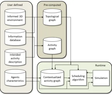
Figure 1: Structure of the scheduling model.
[FBT99, TD00, MM10] which have been extended to associate crowd behaviours with parts of the environment [SGC04]. In such approaches, the topology and the nature of the environment are taken into account but there is no explicit relation with activity scheduling.
Crowd distribution in cities depends on the way people schedule their daily tasks. In the field of geosimulation, the MAGS project [MCP∗03] and extensions [ML10] use multi-agent systems to model crowds activity. In this approach, each agent has a given set of goals to satisfy and the whole simulation can be driven by a user specified scenario [KSRF11]. Paris et al. use the concept of affordance [Gib79] in order to generate activity driven navigation [PD09]. But this action selection process relies on a purely symbolic scheme and does not account for spatial knowledge. In this case, the decisional process drives the path planning process but does not model the interrelation between path planning, action selection and scheduling.
In the field of robotics, mixing navigation and mission fulfilment is fundamental. Williams et al. use Temporal Plans Networks to drive a Rapidly exploring Random Tree path planning [WKH∗01]. In his work, Smith et al. generates optimal robot paths satisfying high level mission specifications [STBR11]. His model plans a path in a graph which is the product of a roadmap that represents the environment and a linear Temporal Logic Graph that specifies the mission parameters. This approach focuses on shortest path computation and does not take into account explicit time constraints or any criteria specific to human behaviour such as individual preferences.
At last, in the field of combinatorial optimization, the traveling salesman problem has been extensively studied [Kru56]. This problem emphasizes on the complexity of determining an optimized path that visits a set of positions in a graph. This problem is quite similar to the one we address in this paper. However, in our approach, we add more constraints such as explicit temporal constraints, activity scheduling, and take into account agent personal preferences.
Comparison with previous work. Compared to previous work, our model better handles the tight relationship between intended activity, time and space. An agent intended activity can be described independently of the environment. Indeed, the proposed scheduling algorithm will automatically choose adequate locations where tasks should be performed. For people interested in evaluating flows of pedestrians inside a virtual prototype of an environment layout, a complex behaviour model is not required as our algorithm produces sufficient information to run a simulation based on our scheduling model coupled with a reactive navigation process. We also confronted our algorithm to human produced schedules. Results show that our model produces tasks schedules that mostly reflect human ones.
3
Model overview
Knowing what an agent intends to do within a given time interval, our model aims at scheduling a set of tasks and choosing locations where those tasks will be performed. The proposed scheduler produces a task schedule that optimizes
an effort function and respects spatial and temporal constraints that have been provided. Our model relies on three inputs:
• An informed environment description is used for three purposes. First, it aims at describing the environment topology. It qualifies the accessibility between different locations and is used to estimate travel distances between locations. Second, it contains information about tasks that can be performed by the agents and their location. Last, the same representation is used to handle the simulation phase and more precisely the navigation of the agents. • An agent description depicts characteristics specific to this agent, such as its accepted navigation speeds, estimated
effort associated to these speed and to waiting time.
• An intended activity description, which describes a set of tasks, the possible orderings of these tasks, as well as spatial and temporal constraints relating to these tasks.
Based on these environment description, agent characteristics and intended activity description, a scheduling algorithm computes a valid task schedule. This task schedule respects spatial and temporal constraints imposed by the intended activity description. A location and an estimated starting time are associated to each task. The location is either the location provided in the intended activity description or a location that has been chosen by the scheduling algorithm. Tasks estimated starting times respect temporal constraints imposed by the opening hours of the chosen locations as well as those provided in the intended activity description. Finally, this task schedule optimizes an effort function that is used to guide the search for a solution. This effort function valuates the effort relating to predicted navigation speeds, travelled distances, waiting times and task realization and consequences. Temporal constraints associated to the produced task schedule are finally relaxed into time intervals. This relaxation is based on the intended activity temporal constraints and opening hours associated to the different tasks locations. The simulated agent is then provided with this relaxed task schedule. During the simulation phase, the agent moves from place to place to perform its activity and uses the relaxed temporal constraints to estimate if it is late or not and possibly adapt its navigation speed accordingly . In this article, we mainly focus on the proposed scheduler and on the task schedule relaxation.
4
The agent and the environment
In this section, we discuss the environment representation, the agent characteristics and the description of an intended activity. Those three components are the input of the proposed scheduling algorithm that is presented in the next section. In this section, we focus on the pieces of information required by our scheduling algorithm and voluntarily omit some simulation-related informations.
4.1
Informed environment
Information process and associated data. To ease the environment design process, the environment representation is computed from an informed 3D geometry of the environment in which the simulation will occur. The information process is achieved by assigning a unique identifier to groups of geometries that share the same functionalities from the simulation point of view. These identifiers refer to a database that describes the properties associated with the groups of geometries: a location type and opening hours. The location type refers to a set of tasks that can be performed at the associated location. For instance, the location type can be a bakery in which tasks ”buy bread” and ”buy dessert” can be performed. The opening hours characterize time intervals during which tasks can be performed at the given location. A second part of the database is dedicated to the description of tasks characteristics: an estimated duration, an effort cost and an effort penalty. The estimated duration is a function of time that models the common knowledge about attendance. The effort cost expresses the effort spent in performing the task. The effort penalty acts as a modifier of the effort related to navigating and performing the remaining tasks. For instance, if somebody buys goods, he has to carry some bags, which implies a greater effort during navigation as well as a discomfort when performing other tasks.
Environment precomputation. The environment representation is automatically extracted from the geometry by using a spatial analysis process similar to the one presented in [Lam09]. An exact 3D subdivision of the geometry is computed and a 2D map of the environment (a constrained Delaunay triangulation [Kal05, LD04]) is extracted. During the whole process, the links to the information database are kept. That way, the navigation area of each location of interest is identified in the 2D map. A roadmap, which is a coarse approximation of the generalized Vorono diagram of the 2D map, is also extracted. An abstraction of this roadmap will be used to estimate travel distances between different locations in the environment.
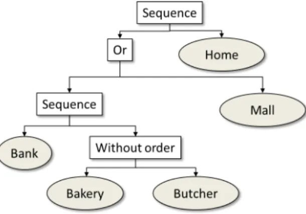
Figure 2: A hierarchical description of an intended activity.
4.2
Agent characteristics
A set of paces (walking, hurrying and running for instance) is associated to each agent. A pace is characterized by a navigation speed and a cost. The cost symbolizes the effort implied by using the corresponding navigation speed. The higher the cost, the less likely the agent uses the pace in a task schedule. A waiting cost is also assigned to the agent. It allows evaluating if the agent is prone to wait (low value) or on the contrary is prone to do other things instead of waiting, even if it implies that it will have to hurry to be on time (high value). A wide variety of agents archetypes, representing categories of population, can be described with those parameters.
A set of agent specific locations is also associated with each agent. The purpose of these locations is to constrain the intended activity description in order to follow some logic related to the agent ”life”. For instance, an agent is especially associated with one home: the one he inhabits. To decouple the agent description and the simulation environment, locations are randomly chosen accordingly to their type (workplace, dwelling place). Some statistical data can be used to favour some locations choices to others depending on the agent. For instance, it can reflect the fact that, by contrast with flats, houses are more likely to be populated with families or elderlies than with students.
4.3
Modelling agent intended activity
The aim of our model is to intelligently schedule tasks that an agent intends to perform. The agent intended activity is modelled by using a hierarchical description based on the notions of tasks, activities and constructors (operators that describe how tasks and activities can be combined). It focusses on what the agent intend to do and the possibly associated constraints (ordering, locations and dates). In our model, a task is atomic and can be performed in an appropriate place at an appropriate time. Activities are combinations of tasks or activities. An activity description aims at describing all possible realization variants in terms of valid tasks sequences. To ease the description of all those variants, we use the following constructors: sequence, either (choice of one sub-activity), without order and interlace that combines activities by interlacing them at the task level. Those constructors provide the user with an expressive tool that can be used to describe very complex activities. For instance, without order and interlace operators enable to describe an activity that can be achieved in many possible ways. An example of such description is provided Fig. 2.
When used to describe an agent intended activity, tasks can be constrained with a location and a time interval. If no location constraint is provided, the place will be automatically chosen among all appropriate ones. Otherwise, the provided one will be used. The time interval constraint implies that the associated task must start within the given time interval. This can be used to model working hours or appointments for instance. If no temporal constraint is given, the task can be performed anytime during the opening hours of the provided / chosen location. Temporal constraint can also be applied to an activity. This implies that all tasks compounding this activity will have to start within the associated temporal constraint.
5
Task scheduling algorithm
The proposed task scheduling algorithm combines the topology of the environment with the intended activity description in order to compute a sequence of instantiated tasks (tasks with associated location and starting time) that respects
n0 n1 n2
n3 n4 n5
n6
work bank butcher
mall
bakery home
Figure 3: Example of a topological graph.
s0 s1 s2 s3 s4 –S–sf bank mall bakery butcher butcher bakery home
Figure 4: The activity graph built from the description given in Fig. 2.
spatial and temporal constraints provided by the intended activity description. The produced tasks sequence minimizes an effort function that takes into account the estimated distance between the different locations, the estimated navigation speeds, the waiting time and the effort associated to performing a task. The exploration space associated to the algorithm is the product of the locations in the environment, the progress in the intended activity, the time and the speeds used to navigate from one place to another. To lower the size of this exploration space, we compute optimized data structures: the topological graph and the activity graph. After presenting these data structures, we describe the main steps of our algorithm. Finally, the relaxation of the time constraints associated to the computed task sequence is discussed.
5.1
Topological graph
The topological graph aims at combining the characterization of accessibilities and the identification of locations where tasks can be performed. Its structure is a simplification of the roadmap associated with the environment, augmented with information concerning tasks (see Fig. 3).
The set V of vertices in the topological graph is a subset of the waypoints belonging to the original roadmap. In V , only one waypoint per location where a task can be performed is is kept. Furthermore, among all waypoints belonging to the roadmap and not belonging to a location, only those characterizing crossings (having strictly more than two edges) are kept. Two types of edges are used in the topological graph: navigation edges and task edges. The navigation edges link vertices belonging to V if they were linked with a direct path (a path with no crossings) in the original roadmap; these edges are labelled with the distance (estimated from the original roadmap) between waypoints. Task edges loop on a waypoint symbolising a location and are labelled with the tasks that can be performed at the associated location.
The topological graph is an abstraction of the environment roadmap that only contains useful information: waypoints model either a route choice implied by a crossing or locations where tasks can be performed. This topological graph is used for two different purposes: locating tasks in the environment and estimating the distance between locations where tasks can be performed.
5.2
Building the activity graph
In our model, an activity graph is a state machine which aims at recognizing any sequence of tasks that can be used to perform an intended activity. In this activity graph, states are situations (in term of execution state of an activity) and each transition is labelled with a task that implies the associated situation change. This activity graph is automatically built from the intended activity description. This building process uses two passes: a pre-computation that only depends on the intended activity and a contextualization process that propagates environmental constraints in the activity graph. Pre-computation. During the pre-computation pass, time constraints are propagated in the hierarchical description of the intended activity. Thus time constraints associated with the tasks are the intersection between their own time constraints and those of the constructors belonging to the branch leading to the root of the tree. The activity graph
04. S = best(OP EN ED) 05. if goal(S) then break
06. OP EN ED = OP EN ED n S 07. N = successors(S)
08. f or each S0 ∈ N
09. if !f ilter(S0, CLOSED)∧ !prune(S0) then 10. update(S0, CLOSED)
11. OP EN ED = OP EN ED ∪ S0
12. if OP EN ED = ∅ then F AILU RE 13. Construct schedule f rom best(OP EN ED) 14. Relax constraints on schedule
Figure 5: Task scheduling algorithm.
is then built by translating the intended activity description into a state machine (see Fig. 4). Each constructor used in the intended activity description has its equivalent in terms of state machine construction. For instance, a sequence operator concatenates two state machines; the interlace operator computes a product of several state machines. As the description of the intended activity may not produce an optimal state machine, a minimization algorithm [Hop71] is used. This algorithm guarantees that the computed state machine contains a minimal number of states and paths linking the entry state to the end state.
Contextualization of the activity graph. This second pass aims at propagating constraints related to the envi-ronment in the activity graph. For each task t labelling a transition, the union of opening hours of the associated locations is computed and intersected with the time interval assigned to t. The envelope of the resulting set of time intervals is then assigned to t. This new time interval represent all possible starting dates of the task. Finally, for each situation, we compute a time interval characterizing the possible feasibility of the activity from this situation. Being in this situation but out of this time interval implies that no solution can be found. To compute those intervals, an interval [start time of simulation; maximum time] is associated to the end situation of the activity graph. Other situations are marked as not constrained. Then for each non constrained situation S with transitions leading to constrained situations, the associated time interval is computed. First, for each transition starting from S, the intersection between the time interval associated with the task and the time interval associated with the ending situation is computed. Then, the union of these intervals is computed and the lower bound is replaced by the starting time of the simulation. This final interval is associated to S. To sum up, the built activity graph is minimal. Therefore, two different descriptions of the same activity will lead to the same minimal activity graph structure. This implies that our algorithm is not sensitive to the intended activity description but only to the intrinsic nature of this activity. Time intervals associated to the situations of the activity graph characterize the possible feasibility of the remaining activity and take into account the intended activity constraints coupled with environmental constraints. Those intervals will be used to efficiently prune solution search during scheduling.
5.3
Task scheduling algorithm
Our scheduling algorithm is depicted Fig. 5. It is a variant of the A* algorithm []. It explores a search space that is the product of the nodes in the topological graph, the situations in the activity graph, the paces and the time. In this A* variant, the closed node structure (CLOSED) is not the usual set of exploration states but a dedicated data structure. The algorithm also uses a pruning function which relies on time constraints. In the following, we explain the main aspects of this algorithm. An exploration state contains the node in the topological graph, the situation in the activity graph, the time, the pace, an effort penalty, the effort accumulated form beginning of the activity and an estimation of the remaining effort (heuristic function). The OPENED data structure contains opened exploration states. The best function is used to get the exploration state in OPENED that minimizes the effort summed to the remaining effort.
Successor state generation. In the algorithm, the successors function generates all successor states of the provided state S. A successor state S0 is possibly generated for each edge e connected to the node of the topological graph in S. In the following, we assume that S0is initialized as a copy of S and only describe the modifications. In S0, the node is set to the other extremity of e. The estimated remaining effort is estimated based on the node, the situation and the pace in S0. The computation of other data is handled as follows.
• If e is a navigation edge, time in S0is increased by the time needed to navigate along the path symbolized by e. The effort is increased by the effort spent in navigating along the path. This effort is equal to (l/sp) × (c + p) in which l
is the length of the path, c is the cost associated to the current pace, sp is the speed associated to the current pace and p is the effort penalty in S.
• If e is a task edge, a state S0is created for each available pace. The effort penalty is increased by the effort penalty associated to the task labelling e. Time is increased by the time needed to perform the task. The effort is increased by the effort relating to performing the task. This effort is equal to dt× (et+ p) + dw× ewin which dtis the duration of the task, et is the effort cost of the task, p is the effort penalty in S, dw is the waiting duration and ew is the effort associated with waiting.
During the successor state generation, the agent’s pace cannot change if using navigation edges but only after performing a task. There are at least two reasons for this choice. First, the length of navigation edges is not constant but varies from place to place. Therefore, among two locations at almost equal distance, one location could be favoured just because the agent could better adapt its average speed by using more navigation edges. Second, if a change of pace is allowed each time a navigation edge is used, the number of successor states increases drastically. This leads to higher memory requirements as well as a higher computation time.
Closed nodes structure and filtering. The closed node structure is a three dimensional table (node of the topological graph × situations × pace). Each cell contains a sorted table storing couples (time, effort). In the following, we consider a state S and the table T stored in the cell corresponding to the node, situation and pace in S. In the algorithm, the filter function prunes a state S if ∃C ∈ T such as time(C) ≤ time(S) ∧ ef f ort(C) < ef f ort(S). If S is not pruned, the table T is updated by removing all couple C ∈ T such as time(C) ≥ time(S) ∧ ef f ort(C) < ef f ort(S). The couple (time(S), ef f ort(C)) is then inserted in T .
Exploration state pruning. The prune function used in the algorithm uses the time constraints to filter states characterizing situations that lead to infeasible task schedules. To do so, the time associated to the tested exploration state is compared to the time constraints associated to the current situation in the activity graph. If this time does not lie in the time interval associated to the situation, the state is pruned as the situation cannot lead to a feasible task schedule. Estimation of the remaining effort. The estimation of the remaining effort is used as a heuristic function to guide the search for a solution. The remaining effort is estimated by estimating the effort associated to performing the remaining tasks and the effort associated to navigating from one place to another.
The estimated effort related to performing the remaining tasks is computed once for all and the estimation is associated to each situation of the activity graph. First, a minimal effort value is associated to each task labelling a transition of the activity graph. This minimal effort value is computed from the original task description. Then the estimation of the remaining effort is computed for each situation as follows. The ending situation of the activity graph is associated an effort value equal to zero (there is no remaining task). For a situation s and for each transition starting from s, an effort value equal to the estimated effort associated to the task labelling the transition summed with the estimated effort value of its ending situation is computed. The situation s is then associated the minimal value among all efforts computed for the transitions.
The estimated remaining effort relating to navigating between different locations where tasks can be performed depends on two factors: the node in the topological graph and the situation in the activity graph. Let note e(p) the effort value associated to pace p and emthe minimal effort associated to the paces. For a given node n of the topological graph and a given situation s of the activity graph, we define a function D(n, s). This function returns a set of couples (d1, d2), one per task t labelling a transition starting from s. In a couple (d1, d2), d1is the minimal distance to a location where t can be performed and d2 is the shortest distance that must be travelled whichever the sequence of tasks performed after t is. The estimated effort value is then computed as follows:
E(n, s, p) = min(d1,d2)∈D(n,s)d1∗ e(p) + (d2− d1) ∗ em
The distance d2is computed as follows. Let Q(s) be the set of all possible remaining tasks sequences when in situation s, T (q) be the set of all tasks in the sequence q and d(t) the distance to the nearest place where task t can be performed. Given a situation s, d2 is computed as follows:
d2= minq∈Q(s)(maxt∈T (q)(d(t)))
In order to lower the computation cost, d(t) is pre-computed for every node of the planning graph and for any possible task t. Furthermore, when evaluating d2, we store intermediate results in a cache for later use. This cache associates a d2 value to each couple (s, n) for which this value has been computed. This greatly enhances the performances of the heuristic computation.
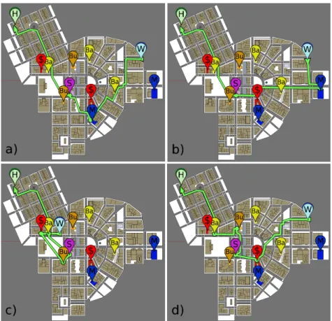
Figure 6: Intended localised task sequence for a parent worker leaving work at 4:15 pm, (a) with our model and (b) with a reactive model, (c) when changing home location or (d) leaving at 4:25pm.
Task schedule and constraint relaxation. From the sequence of states from best(OPENED) to the initial state, the task schedule {t0, ..., tN} is extracted. In this task schedule, tasks t0 is a zero duration task symbolizing the initial state of the agent. Tasks t1 to tN are the tasks selected from the intended activity description. Starting times associated to each task are the earliest given the chosen navigation paces. However, as this schedule will be performed by an agent navigating in a crowded environment, dates are indicative but will not be precisely respected. To give more freedom to the agents, time constraints are relaxed by assigning starting time intervals to each task. Let S(t) be the start time of task t, F(t) be the finish time of t, d(t) be the duration of t (without waiting time), O(t) be the set of opening time intervals of the location where t is performed and E (I) be the envelope of a set of intervals I. We define the relaxed time constraint (a.k.a. the interval during which the task can be started) R(tk) = [R(tk); R(tk)] of a task tk in {t0, ..., tN} as follows:
R(tN) = E(O(tN) ∩ [S(tN); +∞])
R(tk) = E(O(tk) ∩ [S(tk); R(tk+1) + S(tk+1) − F (tk) − d(tk)])
If a task is started within its associated time interval, the agent will normally be able to perform the remaining tasks in time. We use the term normally because, as in real life, external factors may prevent the agent from correctly performing the scheduled tasks.
6
Results
To test our model and its correlation with humans decisions, we created a 3D model of a city centre. This 3d model features an elementary school, two malls, two banks, three bakeries, two butchers as well as several houses and workplaces. Agents and humans were given three different paces: walking, hurrying and running. The agents and humans were assigned the following activity: leave work and go back home. On the way to home, some food must be bought, either by going to the mall or by getting some money at a bank and then going, in any order, to the bakery and the butcher.
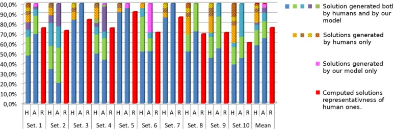
Figure 7: Statistical repartition of different localised task sequences provided by the experiment participants (H) and automatically generated by our algorithm (A) for ten setups. Computed representativeness of computed results (R). (note that identical task sequences are represented by the same colour between columns H and A of one setup, not between different setups.
Moreover, children must be picked at school at 4:30pm. At any time, agents or humans can go home to get rid of all the shopping bags. In the following, we discuss the properties of our scheduling algorithm and compare its results to tasks schedules produced by humans.
6.1
Activity scheduling properties
Fig. 6 depicts task schedules obtained in different situations.
In cases (a) and (b), we compare our algorithm (a) to a reactive algorithm that does not use look-head capabilities (b). In this example, the agent leaves work at 4:15pm. In both cases, the agents choose to visit a mall before going to the school. However, our algorithm chooses the mall closest to the school, even if the path is longer. Indeed, the agent spends less time carrying goods. Such an example demonstrates the impact of a long term decision and the effort penalty associaed to tasks description.
In Fig. 6(c), compared to case (a), we only changed the initial location of the agent. This change does not only impact the choice of locations but also the performed tasks. In that case, the task sequence has been optimized, allowing the agent to visit the bank and butcher before going to school and without being late. Such a result results from the combination of spatial and temporal constraints with long term scheduling.
Finally, in Fig. 6(d), we show the impact of time constraints. In this case, the agent leaves work at 4:25pm instead of 4:15pm. Our algorithm detects that there is not enough time to go to the mall. However, the agent, if hurrying, can to the bank to get some cash before taking is children at school. Finally, it visits the bakery and butchery. Indeed, even if a faster pace implies a greater immediate cost, the agent avoids a later detour which would have increased the global cost of the task schedule.
6.2
Task scheduling model evaluation
In order to validate the representativeness of our task scheduling model, we carried out an experiment aiming at comparing the output of our algorithm to human-generated schedules. To do so, we provided 31 participants with 10 maps describing 10 activity scheduling setups with different starting time, workplace and home location. The provided environment and activity where the same as in the previously discussed examples. In each setup, when combining possible task sequences with locations, we obtain 438 potential solutions. We provided the participants with three rulers indicating the approximate time needed to travel given distances if walking, hurrying or running. Participants were asked to indicate the locations they would intend to visit in order to perform the activity if in a similar real-life situation.
For each setup, the experiment results were grouped by intended task schedules. In Fig. 7, the ”H” columns depicts the statistical repartition of human task schedules for every setup. In the general case, one main solution could be identified, as well as few secondary ones. The remaining answers were scattered. Among our 10 setups, the percentage of main solutions ranges from 34.6% to 91.7 % of the total answers, with a mean of 58.4%. The two principal solutions reach
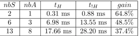
6 3 6.98 ms 13.55 ms 48.5%
13 8 17.66 ms 28.20 ms 37.4%
Table 1: Performance of our algorithm for three activity graphs consisting of nbS situations and nbA possible task sequences: tH with estimated effort and t!H without; gain, mean gain for using the estimated effort.
75.6% of the answers, and goes up to 87.1% for the three principal ones. However, in every case, some alternative solutions were proposed. These solutions represent a mean of 12.9% of participants’ answers. This demonstrates a variability in humans’ activity scheduling. However some shared tendencies can be observed.
After the experiment, we asked the participants to answer some questions about their global preferences (Do you prefer shopping in malls or in small shops? How do you feel about waiting for ten minutes?...). From the set of fulfilled forms, a statistical repartition of agents’ parameters values (cost associated with tasks, pace cost, waiting time cost and effort penalty) has been computed (independently of human provided tasks schedules). We then created a set of 1000 agents parameterized by values randomly picked with a probability distribution matching those statistics. This set was used as an input to our algorithm in order to schedule the activity in the 10 setups provided to participants. The generated solutions were grouped and matched with the group of human-planned ones, see columns ”A” in Figure 7.
The statistical repartition of computed solutions is very similar to the observed one. In most of the setups (except setup 2), the main solution provided by our algorithm is the same as the main solution provided by the participants. We can also observe that most of secondary solutions were also generated: only a mean of 19.3 % of human-generated solutions were never generated by our algorithm. Those non-generated solutions imply a greater effort whatever the parameters of our algorithm are. This can be explained by the fact that people tend to use a path globally directed to the goal, even if this path is longer. On the opposite, less than 4% of generated solutions corresponded to no human-planned solutions. In column ”R” of Fig. 7, a representativeness value is depicted. This value is defined by the intersection of statistical distributions of tasks schedules generated by humans and those generated by our algorithm. This value represents the capability of our algorithm to generate populations with tasks schedules corresponding to humans ones. Over our 10 test setups, we obtained between 64.0% and 95.4% of representativeness, with a mean of 76.4%. This demonstrates that, given a coherent distribution of personal preferences, our algorithm is capable of generating representative tasks schedules that take into account human variability through parameterization.
6.3
Performance evaluation.
As we intend to use this algorithm in real-time applications, it is essential to keep the computation times reasonable. The Table 1 sums up the mean computation time average for 1000 planning calls in a 5754 nodes planning graph, using activity graphs of increasing complexity. Columns tH and t!H show the algorithm performances with and without the proposed heuristic. We observe that the performances are highly correlated to the number of possible arrangements nbA in the activity graph. These values are acceptable for real-time applications, but can become a problem with a more complex activity graph.
6.4
Crowd simulation
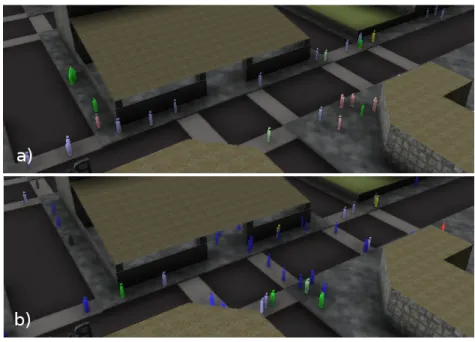
We used this model to populate our virtual urban environment with 10000 agents embedded with activities randomly selected from a small set of activity graphs. These agents were generated in real-time from 4 pm to 4.20 pm and animated along the planned path using a path optimization and a collision avoidance system inspired by the work in [LD04, vdBLM08, OPOD10]. By using the relaxed constraints on the computed activity schedules and possibly a partial rescheduling in case of detected potential failure, the agents were able to perform their activity. Some macroscopic crowd phenomenon emerged in the city. For instance, we could observe some flows going from the work areas to the housing areas, and higher densities of pedestrians appearing in front of the school around 4.30 pm. As an example, Figure 8 shows the difference between obtained flows in front of the school at 4.10 pm and 4.20 pm. This shows how our model can be used to populate virtual environment with consistent densities of pedestrians.
Figure 8: Population in front of the school at 4.10 pm (a) and 4.20 pm (b). In b, a strong flow of people going to the school appears, that did not exist in a.
Conclusion
In this paper, we presented an original task scheduling process taking into account a description of an environment, of an agent characteristics and of its intended activity. This process aims at selecting where, when and in which order several tasks, representing an intended activity, should be performed. The proposed model handles spatial constraints as well as temporal constraints. The agent’s personal preferences are also taken into account in the scheduling process. Produced task schedules are optimized on the long term and exhibit adequate choices of locations and times with respect to the agent intended activity and its environment. We validated our scheduling algorithm results with an experiment. This experiment showed variability in human’s generated schedules. However, our scheduler was able to produce tasks schedules that are representative of humans’ ones in 76.4% of our test cases.
Future work will focus on three aspects. First, we intend to extend the model to handle hierarchical representations of environments and activities. This will enhance the algorithm performances while enabling a more precise description of activities. Second, we plan to make our algorithm reactive to unexpected failures (missing an appointment for instance) or opportunities (finding an unknown bakery for instance). Finally, we plan to enhance our validation process through the comparison with measured flows and densities in a real city. However, given the nature of our problem, designing such a validation process is a research issue on its own. It requires gathering data on a large population (activities, agendas, paths) during long time periods in a large environment. It also implies to deal with privacy issues related to such an experiment.
References
[DAPB08] Durupinar F., Allbeck J., Pelechano N., Badler N.: Creating crowd variation with the ocean personality model. In AAMAS (2008), pp. 1217–1220.
[FBT99] Farenc N., Boulic R., Thalmann D.: An informed environment dedicated to the simulation of virtual humans in urban context. CGF 18, 3 (1999), 309–318.
[Gib79] Gibson J. J.: The Ecological Approach to Visual Perception. Lawrence Erlbaum Associates, 1979, ch. The Theory of Affordances, p. 127 143.
[HB04] Hoogendoorn S. P., Bovy P. H. L.: Pedestrian route-choice and activity scheduling theory and models. Transportation Research Part B: Methodological 38, 2 (February 2004), 169–190.
[JIG13] Jaklin N. S., IV A. F. C., Geraerts. R.: Real-time path planning in heterogeneous environments. In CASA (2013).
[JL11] Jørgensen C. J., Lamarche F.: From geometry to spatial reasoning: automatic structuring of 3d virtual environments. Motion In Games (2011).
[Kal05] Kallmann M.: Path planning in triangulations. In Workshop on Reasoning, Representation and Learning in Computer Games (2005).
[Kit04] Kitazawa K.and Batty M.: Pedestrian behaviour modelling. In Proc. of International Conference on Design and Descision Support Systems in Architecture and Urban Planning (2004).
[Kru56] Kruskal J. B. J.: On the shortest spanning subtree of a graph and the traveling salesman problem. In American Mathematical Society (1956).
[KSRF11] Kapadia M., Singh S., Reinman G., Faloutsos P.: A behavior-authoring framework for multiactor simulations. Computer Graphics and Applications 31, 6 (2011), 45–55.
[LA11] Li W., Allbeck J.: Populations with purpose. Motion in Games (2011), 132–143.
[Lam09] Lamarche F.: Topoplan: a topological path planner for real time human navigation under floor and ceiling constraints. In CGF (2009), vol. 28, pp. 649–658.
[LCHL07] Lee K., Choi M., Hong Q., Lee J.: Group behavior from video: a data-driven approach to crowd simulation. In SCA (2007), pp. 109–118.
[LD04] Lamarche F., Donikian S.: Crowd of virtual humans : a new approach for real time navigation in complex and structured environments. CGF 23 (2004), 3.
[LDA12] Li W., Di Z., Allbeck J.: Crowd distribution and location preference. Computer Animation and Virtual Worlds (2012).
[MCP∗03] Moulin B., Chaker W., Perron J., Pelletier P., Hogan J., Gbei E.: Multi-agent geosimulation and crowd simulation. In Conf. On Spatial Information Theory (2003).
[ML10] Moulin B., Larochelle B.: Modelling, Simulation and Identification. InTech, 2010, ch. CrowdMAGS: Multi-agent geo-simulation of the interactions of a crowd and control forces, pp. 213–237.
[MM10] Mekni M., Moulin B.: Motion planning of autonomous agents situated in informed virtual geographic environements. Int. Conf. on Advanced Geographic Information Systems, Applications and Services (2010). [OPOD10] Ondrej J., Pettr J., Olivier A.-H., Donikian S.: A synthetic-vision-based steering approach for
crowd simulation. In SIGGRAPH ’10 (2010).
[PD09] Paris S., Donikian S.: Activity-driven populace: a cognitive approach for crowd simulation. Computer Graphics and Applications 29 (2009), 34–43.
[SGC04] Sung M., Gleicher M., Chenney S.: Scalable behaviors for crowd simulation. In CGF (2004), vol. 23, Wiley Online Library, pp. 519–528.
[SGG∗07] Sud A., Gayle R., Guy S., Andersen E., Lin M., Manocha D.: Real-time Simulation of Heterogeneous Crowds. Tech. rep., University of north california, 2007.
[ST05] Shao W., Terzopoulos D.: Autonomous pedestrians. In SCA (2005), pp. 19–28.
[STBR11] Smith S., Tumova J., Belta C., Rus D.: Optimal path planning for surveillance with temporal-logic constraints. Int. Journal of Robotics Research 30, 14 (2011), 1695–1708.
[TD00] Thomas G., Donikian S.: Modelling virtual cities dedicated to behavioural animation. CGF 19, 3 (2000), 71–80.
[TD07] Thomas R., Donikian S.: A spatial cognitive map and a human-like memory model dedicated to pedes-trian navigation in virtual urban environments. Spatial Cognition V Reasoning, Action, Interaction (2007), 421–438.
[TDOP01] Turner A., Doxa M., O’Sullivan D., Penn A.: From isovists to visibility graphs : a methodology for the analysis of architectural space. Planning and Design 28 (2001).
[vdBLM08] van den Berg J., Lin M. C., Manocha D.: Reciprocal velocity obstacles for real-time multi-agent navigation. In ICRA (2008).
[vTIG11] van Toll W. G., IV A. F. C., Geraerts R.: Navigation meshes for realistic multi-layered environments. In ICRA (2011).
[WKH∗01] Williams B., Kim P., Hofbaur M., How J., Kennell J., Loy J., Ragno R., Stedl J., Walcott A.: Model-based reactive programming of cooperative vehicles for mars exploration. In Int. Symp. Artif. Intell., Robotics, Automation Space (2001).
[YCP∗08] Yeh H., Curtis S., Patil S., van den Berg J., Manocha D., Lin M.: Composite agents. In SCA (2008), pp. 39–47.