On the most imbalanced orientation of a graph

HAL Id: hal-01497825

https://hal.archives-ouvertes.fr/hal-01497825

Submitted on 29 Mar 2017

HAL is a multi-disciplinary open access

archive for the deposit and dissemination of

sci-entific research documents, whether they are

pub-lished or not. The documents may come from

teaching and research institutions in France or

abroad, or from public or private research centers.

L’archive ouverte pluridisciplinaire HAL, est

destinée au dépôt et à la diffusion de documents

scientifiques de niveau recherche, publiés ou non,

émanant des établissements d’enseignement et de

recherche français ou étrangers, des laboratoires

publics ou privés.

On the most imbalanced orientation of a graph

Walid Ben-Ameur, Antoine Glorieux, José Neto

To cite this version:

Walid Ben-Ameur, Antoine Glorieux, José Neto. On the most imbalanced orientation of a graph.

COCOON 2015 : 21st International Conference on Computing and Combinatorics, Aug 2015, Beijing,

China. pp.16 - 29, �10.1007/978-3-319-21398-9_2�. �hal-01497825�

On the most imbalanced orientation of a graph

Walid Ben-Ameur, Antoine Glorieux, and Jos´e Neto

Institut Mines-T´el´ecom, T´el´ecom SudParis, CNRS Samovar UMR 5157 9 Rue Charles Fourier, 91011 Evry Cedex, France

walid.benameur@telecom-sudparis.eu,antoine.glorieux@telecom-sudparis.eu, jose.neto@telecom-sudparis.eu

Abstract. We study the problem of orienting the edges of a graph such that the minimum over all the vertices of the absolute difference between the outdegree and the indegree of a vertex is maximized. We call this minimum the imbalance of the orientation, i.e. the higher it gets, the more imbalanced the orientation is. We study this problem denoted by MAXIM. We first present different characteriza-tions of the graphs for which the optimal objective value of MAXIMis zero. Next we show that it is generally NP-complete and cannot be approximated within a ratio of1₂+ ε for any constant ε > 0 in polynomial time unless P = NP even if the minimum degree of the graph δ equals 2. Finally we describe a polynomial-time approximation algorithm whose ratio is almost equal to1₂.

Introduction and notation

Let G = (V, E) be an undirected simple graph, we denote by δG the minimum degree

of the vertices of G. An orientation Λ of G is an assignment of a direction to each undirected edge {uv} in E, i.e. any function on E of the form Λ ({uv}) ∈ {uv, vu}, ∀{uv} ∈ E. For each vertex v of G we denote by d_G(v) or d(v) the unoriented degree of vin G and by d+

Λ(v) or d

+_{(v) (resp. d}− Λ(v) or d

−_{(v)) the outdegree (resp. indegree) of v}

in G w.r.t. Λ . Graph orientation is a well studied area in graph theory and combinatorial optimization and thus a large variety of constrained orientations as well as objective functions have been considered so far.

Among those arise the popular degree-constrained orientation problems: in 1976, Frank & Gy´arf´as [12] gave a simple characterization of the existence of an orientation such that the outdgree of every vertex is between a lower and an upper bound given for each vertex. Asahiro et al. in [1,2,3] proved the NP-hardness of the weighted version of the problem where the maximum outdegree is minimized, gave some inapproxima-bility results, and studied similar problems for different classes of graphs. Chrobak & Eppstein proved that for every planar graph a 3-bounded outdegree orientation and a 5-bounded outdegree acyclic orientation can be constructed in linear time [6].

Other problems involving other criterion on the orientation have been studied such as acyclicity, diameter or connectivity. Robbins’ theorem (1939) for example states that the graphs that have strong orientations are exactly the 2-edge-connected graphs [18] and later (1985), Chung et al. provided a linear time algorithm for checking whether a graph has such an orientation and finding one if it does [7]. Then in 1960, Nash-Williams generalized Robbin’s theorem showing that an undirected graph has a k-arc-connected orientation if and only if it is 2k-edge-k-arc-connected [17]. The problem called

oriented diameter that consists in finding a strongly connected orientation with mini-mum diameter was introduced in 1978 by Ch´vatal & Thomassen: they proved that the problem is NP-hard for general graphs [8]. It was then proven to be NP-hard even if the graph is restricted to a subset of chordal graphs by Fomin et al. (2004) who gave also approximability and inapproximability results [10].

For an orientation Λ of G = (V, E) and a vertex v we call |d_Λ+(v) − d_Λ−(v)| the im-balanceof v in G w.r.t Λ and thus we call minv∈V|d_Λ+(v) − d_Λ−(v)| the imbalance of Λ .

Biedl et al. studied the problem of finding an acyclic orientation of unweighted graphs minimizing the imbalance of each vertex: they proved that it is solvable in polynomial time for graphs with maximum degree at most three but NP-complete generally and for bipartite graphs with maximum degree six and gave a 13₈-approximation algorithm [5]. Then K´ara et al. closed the gap proving the NP-completeness for graphs with maximum degree four. Furthermore, they proved that the problem remains NP-complete for planar graphs with maximum degree four and for 5-regular graphs [14].

Landau’s famous theorem [15] gives a condition for a sequence of non-negative in-tegers to be the score sequence or outdegree sequence of some tournament (i.e. oriented complete graph) and later, Harary & Moser characterized score sequences of strongly connected tournaments [13]. Analogous results for the “imbalance sequences” of di-rected graphs are were given by Mubayi et al. [16]. In 1962, Ford & Fulkerson charac-terized the mixed graphs (i.e. partially oriented graphs) which orientation can be com-pleted in a eulerian orientation, that is to say, an orientation for which the imbalance of each vertex equals zero [11]. Many other results related to orientation have been proposed. Some of them are reviewed in [4].

Let us denote by−→O(G) the set of all the orientations of G, we consider the problem of finding an orientation with maximized imbalance:

(MAXIM) MAXIM(G) = max Λ ∈−→O(G) min v∈V|d + Λ(v) − d − Λ(v)|

and we call MAXIM(G) the value of MAXIMfor G. The minimum degree δGof a graph

Gis a trivial upper bound for MAXIM(G).

The rest of this paper is organized as follows. In the first section, we give several characterizations of the the graphs verifying MAXIM(G) = 0. In section 2, we will show that MAXIMis generally NP-complete even for graphs with minimum degree 2 and inapproximable within a ratio 1₂+ ε for any constant ε > 0 and then will give an approximation algorithm whose ratio is almost equal to 1₂. Since the value of MAXIM

for a graph is the minimum of the values of MAXIMon its connected component, from here on in, all the graphs we consider are assumed to be connected. For any graph G we will use the notations V (G) and E(G) to refer to the set of vertices of G and the set of edges of G respectively.

1

Characterizing the graphs for which M

I

(G) = 0

Now we ask ourselves which are the graphs verifying MAXIM(G) = 0. We will start by unveiling several necessary conditions and properties of such graphs. First we can show

that concerning such a graph, we can find an orientation satisfying several additional properties.

Proposition 1 Let G be a graph such that MAXIM(G) = 0 and u ∈ V . Then there exists an orientation Λ ∈−→O(G) such that u is the only vertex of G with imbalance equal to zero w.r.t. Λ .

Proof. Let Λ ∈−→O(G) be an orientation minimizing |{v ∈ V /|d_Λ+(v) − d−

Λ(v)| = 0}|. We

suppose that |{v ∈ V /|d+

Λ(v) − d −

Λ(v)| = 0}| ≥ 2. We choose two distinct vertices v and

win {v ∈ V /|d+

Λ(v) − d −

Λ(v)| = 0} and a path p = (v = u0, · · · , un= w) between v and

w. If we switch the orientation of the edge {u0u1}, then the imbalance of u0becomes

positive and necessarily the imbalance of u1becomes zero otherwise the resulting

ori-entation would contradict the minimality of Λ . Using the same reasoning, if we switch the orientation of all the edges {u0u1}, · · · , {un−2un−1}, we obtain an orientation where

both un−1and unhave an imbalance equal to zero while the imbalance is positive on all

the vertices u0, · · · , un−2and unchanged on all other vertices. So now if we switch the

orientation of the edge {un−1un} as well, then the resulting orientation contradicts the

minimality of Λ . Hence, |{v ∈ V /|d_Λ+(v) − d−

Λ(v)| = 0}| = 1.

Now let v be this unique vertex of G such that |d_Λ+(v) − d−

Λ(v)| = 0. Let u 6= v be an

arbitrary vertex and let p = (v = u0, · · · , un= u) be a path between v and u. By switching

the orientation of all the edges {u0u1}, · · · , {un−2un−1}, we obtain an orientation Λ0

where u has an imbalance equal to zero while the imbalance is positive for u0 and

unchanged on all other vertices. ut

This yields the following necessary condition: if G is a graph such that MAXIM(G) = 0, then G is eulerian. For let u ∈ V , we know there exists Λ ∈−→O(G) such that {v ∈ V/|d_Λ+(v) − d_Λ−(v)| = 0} = {u}. Then d_Λ+(u) = d_Λ−(u), hence d(u) = d_Λ+(u) + d_Λ−(u) = 2d_Λ+(u) is even. The following lemma about eulerian graphs will prove useful for the proof of our characterization.

Lemma 2 If G is an eulerian graph, then there exists an elementary cycle (hereafter just called cycle) C of G such that G − E(C) has at most one connected component that is not an isolated vertex.

Proof. Being G eulerian and connected, it can be decomposed into edge-disjoint cycles that we can order C1, · · · ,Cnaccording to the following condition: ∪ik=1Ciis connected,

∀i ∈J1, nK. Then Cnis the cycle we are looking for. ut Now let us define a certain family of graphs which will prove to be exactly the graphs for which the optimal objective value of MAXIMis zero. Intuitively they are the graphs for which every block is an odd cycle.

Theorem 3 We define the class of graphsCoddas follows: a simple graph G is inCodd if there exists C1, · · · ,Cnodd cycles (n≥ 1) such that:

• ∪n_i=1Ci= G,

• |V (∪i−1_k=1Ck) ∩V (Ci)| = 1, ∀i ∈J2, nK.

(1)

Proof. • ⇐ We will work by induction on the number of cycles n contained in the graph. Nothing is required for these cycles except that they must be elementary. If n= 1, then our graph is an odd cycle which implies MAXIM(G) = 0. Let n ≥ 2, we assume that all graphs ofCodd _{with k ≤ n − 1 cycles verify MAXIM(G) = 0.}

Let G ∈Codd with n cycles C1, · · · ,Cnas in (1). Suppose there exists Λ ∈

− →

O(G) with strictly positive imbalance. Let us call G0= ∪n−1_i=1Ci the graph obtained from

Gafter removing Cnand let us take a look at Λ|E(G0₎ the orientation of the edges

of G0obtained from Λ as its restriction on E(G0). As G0is a graph of n − 1 cycles inCodd, our inductive hypothesis implies that we have a vertex u ∈ V (G0) such that |d_Λ+

|E(G0)(u) − d

−

Λ_|E(G0)(u)| = 0. Necessarily, u = V (G 0_{) ∩ V (C}

n). Thus |dΛ+(u) −

d_Λ−(u)| = |d+

Λ_|E(Cn)(u) − d −

Λ_|E(Cn)(u)| > 0 implying that MAXIM(Cn) > 0 which is

absurd because Cnis an odd cycle.

• ⇒ Since MAXIM(G) = 0, we know that G is eulerian. We will again work by

induction on the number of cycles n. If n = 1, then our graph is eulerian with a unique cycle, hence it is a cycle. Now as MAXIM(G) = 0, necessarily it is an odd

cycle and is therefore inCodd_{. Let n ≥ 2, we assume that all graphs with k ≤ n − 1}

cycles verifying MAXIM(G) = 0 are inCodd_{. Let G be a graph with n cycles such}

that MAXIM(G) = 0. Thanks to Lemma 2, there exists an cycle C of G such that G− E(C) has at most one connected component G0_{that is not an isolated vertex.}

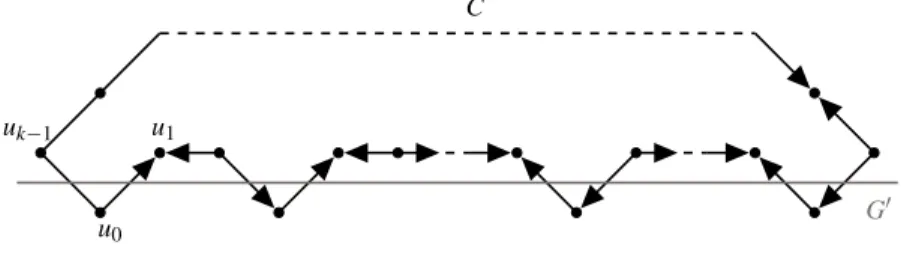
Suppose that MAXIM(G0) > 0, let Λ ∈−→O(G0) with strictly positive imbalance. Let u0∈ V (G0) ∩ V (C), we name the vertices of C as follows: u0, u1, · · · , uk= u0.

Without loss of generality, we can assume that d_Λ+(u0) − dΛ−(u0) > 0; if it was not

the case, replace Λ by its reverse. We complete Λ in an orientation of G by orienting the edges of C: we orient u0u1from u0to u1and go on as follows:

∀i ∈_{J1, k − 1K,} (

if ui∈ V (G0), we orient {uiui+1} as {ui−1ui},

otherwise, we orient {uiui+1} as {uiui−1}.

Where orienting an edge {ab} as another edge {cd} means orienting it from a to bif {cd} was oriented from c to d and from b to a otherwise. Let us have a look at the resulting orientation Λ0 (cf Figure 1): when completing Λ in Λ0, the im-balance of the vertices in V (G0)\{u0} was left unchanged, the imbalance of the

vertices in V (C)\V (G0) equals 2 and the imbalance of u0was either left unchanged

or augmented by two. Hence Λ0has strictly positive imbalance which contraditcts MAXIM(G) = 0, therefore, MAXIM(G0) = 0.

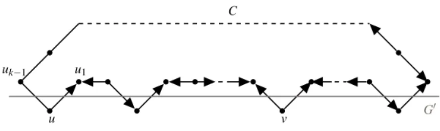
Suppose |V (G0) ∩V (C)| ≥ 2 and let u and v be 2 distinct vertices in V (G0) ∩V (C)) such that u 6= v. Thanks to proposition 1, we know that there exists an orien-tation Λ ∈−→O(G0) such that {w ∈ V /|d_Λ+(w) − d−

Λ(w)| = 0} = {v} and without

loss of generality, d_Λ+(u) − d_Λ−(u) > 0. We name the vertices of C as follows: u= u0u1· · · uk= u0, v = uland we complete Λ in an orientation of G by orienting

the edges of C: we orient {u0u1} from u0and u1and go on as follows:

∀i ∈_{J1, k − 1K \ {l },} (

if ui∈ V (G0), we orient {uiui+1} as {ui−1ui},

And we orient {ulul+1} as {ulul−1}. In the resulting orientation Λ0, the imbalance

of the vertices in V (G0)\{u, v} was left unchanged, the imbalance of the vertices in V (C)\V (G0) equals 2, the imbalance of v was augmented by two and the imbal-ance of u was either left unchanged or augmented by two. Hence Λ0 contradicts MAXIM(G) = 0, therefore, |V (G0) ∩V (C)| = 1.

Suppose C is even. We call u ∈ V (G0) such that V (G0) ∩ V (C) = {u}, and Λ ∈ −

→

O(G0) such that {v ∈ V /|d_Λ+(v) − d_Λ−(v)| = 0} = {u}. We name the vertices of C as follows: u = u0u1· · · uk= u0and we complete Λ in an orientation of G by

orient-ing the edges of C: we orient {u0u1} from u0to u1and {uiui+1} as {uiui−1}, ∀i ∈

J1, k − 1K. In the resulting orientation Λ

0_{, the imbalance of the vertices in V (G}0_)\{u}

was left unchanged, the imbalance of the vertices in V (C)\V (G0) equals 2 and, C being even, the imbalance of u was augmented by two. Hence Λ0 contradicts MAXIM(G) = 0, therefore, C is odd.

As G0is a graph with at most n − 1 cycles verifying MAXIM(G) = 0, by induction

hypothesis, there exist C1, · · · ,Cn−1odd cycles such that:

◦ ∪n−1_i=1Ci= G0,

◦ |V (∪i−1_k=1Ck) ∩V (Ci)| = 1, ∀i ∈J2, n − 1K.

Adding the odd cycle Cn= C, we directly obtain that G ∈Codd.

u t

Fig. 1: The vertices of C in G0are left unchanged imbalance-wise, the other vertices of C are set to 2 and in the end |d+

Λ0(u0) − d − Λ0(u0)| ≥ |d + Λ(u0) − d − Λ(u0)| > 0 . G0 u0 u1 uk−1 C

Now in order to widen our perception of those graphs, let us show another charac-terization.

Theorem 4 For every simple graph G,

G∈Codd_{⇔ G is eulerian with no even cycle}

Fig. 2: The vertices of C in G0are left unchanged imbalance-wise except for v which is set to 2, like the other vertices of C and in the end |d_Λ+0(u0) − d_Λ−0(u0)| ≥ |d_Λ+(u0) − d_Λ−(u0)| > 0 . G0 u v u1 uk−1 C

• ⇐ We will once again work by induction on the number of cycles n.

If n = 1, then our graph is eulerian with a unique odd cycle, hence it is an odd cycle and is therefore inCodd_.

Let n ≥ 2, we assume that all eulerian graphs with no even cycle and k ≤ n − 1 odd cycles are inCodd_{. Let G be a graph with no even cycle and n odd cycles.}

Thanks to Lemma 2, there exists an odd cycle C of G such that G − E(C) has only one connected component G0 that is not an isolated vertex. As G0 is eulerian and even-cycle-free with n − 1 odd cycles, by induction hypothesis, G0∈Codd_{, hence}

there exist C1, · · · ,Cn−1odd cycles such that:

◦ ∪n−1_i=1Ci= G0,

◦ |V (∪i−1_k=1Ck) ∩V (Ci)| = 1, ∀i ∈J2, n − 1K.

Suppose there exist u and v (u 6= v) belonging to V (∪n−1_k=1C_k) ∩ V (C). Since G0 is connected, let p be an elementary path in G0between u and v. We can assume that uand v are the only vertices of C contained in p, otherwise we could replace v by the first vertex of C encountered when travelling on p from u. C defines two other vertex-disjoint paths between u and v: one even that we will call peven and

one odd that we will call podd. p being vertex disjoint with either pevenor podd, by

concatenating it with the one corresponding to its parity, we obtain an even cycle of G, contradicting our hypothesis on G. This yields that |V (C) ∩V (G0)| = 1. From that we can conclude

◦ ∪n i=1Ci= G, ◦ |V (∪i−1_k=1Ck) ∩V (Ci)| = 1, ∀i ∈J2, nK. Hence G ∈Codd_. u t

2

Complexity, inapproximability and approximability

In this section we will prove the NP-completeness and inapproximability of our prob-lem and give an approximation algorithm based on the special case of bipartite graphs. Concerning the complexity of MAXIM, we will show that the problem is NP-complete. More precisely, that answering if MAXIM(G) equals 2 for a graph G such

that δG= 2 is NP-complete. For that purpose we will introduce a variant of the

satis-fiability problem that we will reduce to a MAXIMinstance: the not-all-equal at most

3-SAT(3V).

Not-all-equal at most 3-SAT(3V) is a restriction of not-all-equal at most 3-SAT which is itself a restriction of 3-SAT known to be NP-complete [19] where each clause contains at most three literals and in each clause, not all the literals can be true. Since 2-SAT can be solved in polynomial time, we hereafter deal only with formulas having at least one three-literals clause. The added restriction of not-all-equal at most 3-SAT(3V) is that each variable (not literal) appears at most three times in a formula. The resulting problem is still NP-complete.

Lemma 5 The not-all-equal at most 3-SAT(3V) problem is NP-complete. Proof. See Appendix A.

Now we will associate to a not-all-equal at most 3-SAT(3V) instance ϕ with n vari-ables {x1, · · · , xn} and m clauses {c1, · · · , cm} a graph Gϕ for which the value w.r.t.

MAXIMwill give the answer to whether ϕ is satisfiable or not. If a variable xioccurs

only in positive literals (resp. only in negative literals), it follows that a satisfying as-signment of the variables of ϕ must necssarily give the value TRUE (resp. FALSE) to xi, therefore xican be removed from ϕ with conservation of the satisfiability. Thus,

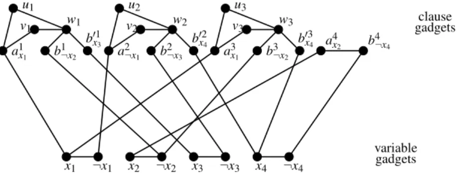
without loss of generality, we can assume that in any not-all-equal at most 3-SAT(3V) formula, every variable occurs at least once as a positive literal and at least once as a negative literal. Gϕ consists of gadgets that mimic the variables and the clauses of ϕ

and additional edges that connect them together:

• the gadget corresponding to a variable xiconsists of two vertices labeled xiand ¬xi

and one edge connecting them;

• the gadget corresponding to a two-literals clause cj= (l1∨ l2), where l1and l2are

its literals, consists in two vertices labeled aj

l1and b

j

l2corresponding to l1and l2

re-spectively (the index ”lk” of the vertices labels stands for the literal they represent, i.e. xiif lkis the variable xiand ¬xiif lkis the negation of the variable xi) and one

edge connecting them;

• the gadget corresponding to a three-literals clause gadget consists in six vertices and six edges. For a clause cj= (l1∨ l2∨ l3), where l1, l2and l3are its literals (the

order is arbitrary), three vertices labeled aj

l1, b

j l2 and b

0 j

l3 correspond to l1, l2and l3

respectively. Three additional vertices are labeled uj, vj and wj and the gadgets’ edges are {aj

l1uj}, {a_lj1vj}, {ujwj}, {vjwj}, {wjb_lj2} and {wjb 0 j l3};

• ∀i ∈_{J1, nK, the vertex labeled x}i(resp. ¬xi) is connected to all the vertices labeled

axji, b j xior b 0 j xi (resp. a j ¬xi, b j ¬xi or b 0 j ¬xi), ∀ j ∈J1, mK. As an example, for a formula

Fig. 3: Gϕfor ϕ = (x1∨ ¬x2∨ x3) ∧ (¬x1∨ ¬x3∨ x4) ∧ (x1∨ ¬x2∨ x4) ∧ (x2∨ ¬x4) x1 ¬x1 x2 ¬x2 x3 ¬x3 x4 ¬x4 a1_x1 b1_¬x2 b01_x3 a2_¬x1 b2_¬x3 b02_x4 a3_x1 b3_¬x2 b03_{x4 a}4 x2 b 4 ¬x4 v1 v2 v3 u1 u2 u3 w1 w2 w3 clause gadgets variable gadgets

the corresponding graph Gϕis represented in Figure 3.

Theorem 6 A not-all-equal at most 3-SAT(3V) formula ϕ is satisfiable if and only if MAXIM(Gϕ) = 2.

Proof. • ⇒ Suppose ϕ is satisfiable and let v : {x1, · · · , xn} → {TRUE, FALSE} be a

satisfying assignment of x1, · · · , xn. We know that δGϕ= 2 which yields MAXIM(Gϕ) ≤

2. So let us build an orientation Λ ∈−→O(Gϕ) which imbalance is greater than or

equal to 2. First, we assign an orientation to the edges of the variable gadget:

Λ ({xi¬xi}) =

(

xi¬xi if v(xi) = TRUE;

¬xixi otherwise.

For example, for the formula ϕ = (x1∨ ¬x2∨ x3) ∧ (¬x1∨ ¬x3∨ x4) ∧ (x1∨ ¬x2∨

x4) ∧ (x2∨ ¬x4) satisfied by the assignment v(x1, x2, x3, x4) = (FALSE, TRUE,

TRUE, TRUE), the edges of the variable gadgets of graph Gϕ are oriented as in

figure 4(a). Since each variable xi occurs at least once as a positive literal and

at least once as a negative literal, 2 ≤ dGϕ(xi) ≤ 3 and 2 ≤ dGϕ(¬xi) ≤ 3, ∀i ∈

J1, nK. Then to ensure our objective on the imbalance of Λ , the orientation of the edges connecting vertex gadgets and clause gadgets must be such that ∀i ∈ J1, nK, |d + Λ(xi) − d − Λ(xi)| = dGϕ(xi) and |d + Λ(¬xi) − d − Λ(¬xi)| = dGϕ(¬xi). In other

words, for i ∈_{J1, nK, if v(x}i) = TRUE (resp. v(xi) = FALSE), then the edges

adja-cent to the vertex xiare oriented from xi(resp. to xi) and the edges adjacent to the

vertex ¬xiare oriented to ¬xi(resp. from ¬xi), e.g. Figure4(b).

So far, all the edges in the variables gadgets and the edges connecting the vertex gadgets and the clause gadgets have been oriented and the vertices in the variables gadgets have imbalance greater than or equal to 2. In order to complete our orien-tation Λ we have to orient the edges in the clause gadgets.

Let cj= (l1∨ l2) be a two-literals clause. Since v satisfies ϕ, we know that exactly

one of the two literals is true w.r.t. v. Which, according to the way we oriented edges so far, means that exactly one of aj

l1 and b

j

Fig. 4: Gϕcorresponding to ϕ = (x1∨ ¬x2∨ x3) ∧ (¬x1∨ ¬x3∨ x4) ∧ (x1∨ ¬x2∨ x4) ∧ (x2∨ ¬x4) satisfied by v(x1, x2, x3, x4) = (FALSE, TRUE, TRUE, TRUE).

x1¬x1x2¬x2x3¬x3 x4¬x4

(x1 ∨ ¬x2 ∨ x3) (¬x1 ∨ ¬x3 ∨ x4) (x1 ∨ ¬x2 ∨ x4)

(x2 ∨ ¬x4)

(a) orientation of the edges in the variable gadgets

x1¬x1x2¬x2x3¬x3 x4¬x4

(x1 ∨ ¬x2 ∨ x3) (¬x1 ∨ ¬x3 ∨ x4) (x1 ∨ ¬x2 ∨ x4)

(x2 ∨ ¬x4)

(b) orientation of the edges between the variable gadgets and the clause gadgets

x1¬x1x2¬x2x3¬x3 x4¬x4

(x1 ∨ ¬x2 ∨ x3) (¬x1 ∨ ¬x3 ∨ x4) (x1 ∨ ¬x2 ∨ x4)

(x2 ∨ ¬x4)

(c) orientation of the edges in the clause gadgets

a variable gadget and the other has one outgoing arc to a variable gadget. If aj

l1

is the one with the incoming arc from a variable gadget (meanings that v(l1) = TRUE), then we assign Λ ({a_lj1b

j l2}) = (b

j l2a

j

l1), otherwise the opposite. We obtain

|d_Λ+(aj l1) − d − Λ(a j l1)| = |d + Λ(b j l2) − d − Λ(b j l2)| = 2.

Let cj = (l1∨ l2∨ l3) (the order is identical to which was chosen to build the

clause gadget, i.e. dGϕ(a

j l1) = 3 and dGϕ(b j l2) = dGϕ(b 0 j l3) = 2) be at three-literals

clause. If the edge connecting aj

l1 to a variable gadget is oriented to a

j

l1 (meanings

that v(l1_{) = TRUE), then we assign Λ ({a}j

l1uj}) = (uja j l1), Λ ({a j l1vj}) = (vja j l1),

Λ ({ujwj}) = (ujwj) and Λ ({vjwj}) = (vjwj). Since v(l1) = TRUE, either both

v(l2) and v(l3) are FALSE or exactly one of v(l2) and v(l3) is TRUE and one is FALSE. If both are FALSE then bj

l2 and b

0 j

l3 have an outgoing arc to a variable

gadget. In that case, we orient wjb_lj2 and wjb 0 j l3 to wj and we obtain |dΛ+(a j l1) − d_Λ−(aj l1)| = 3, |d + Λ(b j l2) − d − Λ(b j l2)| = |d + Λ((b 0 j l3) − d − Λ((b 0 j l3)| = |d + Λ(uj) − d − Λ(uj)| = |d+ Λ(vj) − d − Λ(vj)| = 2 and |d + Λ(wj) − d − Λ(wj)| = 4. If exactly one of v(l 2_{) and}

v(l3_{) is TRUE and one is FALSE, then exactly one of b}j l2 and b

0 j

l3 has an

incom-ing arc from a variable gadget and the other an outgoincom-ing arc to a variable gad-get. If bj

v(l2_{) = TRUE and v(l}3_{) = FALSE), then we assign Λ ({w}

jb_lj2}) = (wjb_lj2) and

Λ ({wjb0 j_l3}) = (b

0 j

l3wj), otherwise the opposite. We obtain |d

+ Λ(a j l1) − d − Λ(a j l1)| = 3 and |d_Λ+(bj l2) − d − Λ(b j l2)| = |d + Λ(b 0 j l3) − d − Λ(b 0 j l3)| = |d + Λ(uj) − d − Λ(uj)| = |d + Λ(vj) − d_Λ−(vj)| = |d_Λ+(wj) − d_Λ−(wj)| = 2.

If, on the other hand, the edge connecting aj

l1 to a variable gadget is oriented

from aj

l1 (meanings that v(l1) = FALSE), then we assign Λ ({a

j

l1uj}) = (a_lj1uj),

Λ ({aj

l1vj}) = (a_lj1vj), Λ ({ujwj}) = (wjuj) and Λ ({vjwj}) = (wjvj). By

sym-metry, we conclude in the same way that |d+

Λ(a j l1) − d − Λ(a j l1)| = 3 and |d + Λ(b j l2) − d_Λ−(bj l2)| = |d + Λ(b 0 j l3)−d − Λ(b 0 j l3)| = |d + Λ(uj)−d − Λ(uj)| = |d + Λ(vj)−d − Λ(vj)| = |d + Λ(wj)− d_Λ−(w_j)| = 2.

Consequently, the imbalance of the resulting orientation Λ is greater than or equal to 2, e.g. Figure 4(c).

• ⇐ Now we assume that MAXIM(Gϕ) = 2, let Λ ∈

− →

O(Gϕ) with optimal imbalance.

Since all the vertices in the variable gadgets have degree at most 3, each vertex xi

(or ¬xi) is necessarily adjacent to only incoming arcs or only outgoing arcs w.r.t. Λ .

We will show that the assignment v : {x1, · · · , xn} → {TRUE, FALSE} of x1, · · · , xn

defined by

v(x_i) = (

TRUE if d_Λ+(xi) > d_Λ−(xi);

FALSE otherwise;

satisfies ϕ. Suppose ϕ doesn’t satisfy a clause cj, j ∈J1, mK. If cjis a two-literals clause (l1∨ l2_{) then either v(l}1_{) = v(l}2_{) = TRUE or v(l}1_{) = v(l}2_{) = FALSE, i.e.}

either both aj

l1 and b

j

l2 have an incoming arc from a variable gadget or both have

an outgoing arc to a variable gadget and in both cases, whichever is the orientation assigned to aj l1b j l2 by Λ , either a j l1 or b j

l2 have a zero imbalance which contradicts

our assumption. So cjis a three-literals clause (l1∨ l2∨ l3) (the order is identical

to which was chosen to build the clause gadget, i.e. dGϕ(a

j l1) = 3 and dGϕ(b j l2) = dGϕ(b 0 j

l3) = 2). Then either v(l1) = v(l2) = v(l3) = TRUE or v(l1) = v(l2) = v(l3) =

FALSE, i.e. either all aj

l1, b

j l2 and b

0 j

l3 have an incoming arc from a variable gadget

or they all have an outgoing arc to a variable gadget. In the first case, it implies Λ ({aj l1uj}) = (uja_lj1), Λ ({a j l1vj}) = (vja_lj1), Λ ({ujwj}) = (ujwj), Λ ({vjwj}) = (vjwj), Λ ({wjb_lj2}) = (wjb j l2) and Λ ({wjb 0 j l3}) = (wjb 0 j l3), and we obtain |d + Λ(wj) −

d_Λ−(wj)| = 0 which contradicts the optimality of Λ . Similarly, in the second case

it implies that the orientations assigned to the edges of the clause gadgets are the opposite from the previous ones and we obtain the same contradiction.

So we can conclude that v does satisfy ϕ.

u t Corollary 7 MAXIMisNP-complete and inapproximable within1_{2+ ε where ε ∈ R}∗₊, unlessP = NP.

Proof. Let ε ∈ R∗+, suppose that there existed a polynomial approximation algorithm

3-SAT(3V) formula and Gϕ its associated graph. Since Gϕcontains at least one

three-literals clause gadget, we know that Gϕcontains an even cycle and δGϕ = 2. This leads

to MAXIM(Gϕ) ∈ {1, 2} and since (1₂+ ε) MAXIM(Gϕ) ≤ val ≤ MAXIM(Gϕ), if the

polynomial approximation algorithm returns a value less than or equal to 1 then (1

2+ ε) MAXIM(Gϕ) ≤ 1 ⇒ MAXIM(Gϕ) < 2 ⇒ MAXIM(Gϕ) = 1;

and if it returns a value greater than 1, then MAXIM(Gϕ) is greater than 1 hence equal

to 2. In other words the polynomial approximation algorithm output answers whether ϕ is satisfiable or not which is absurd unless P = NP. ut

Now we consider the case of bipartite graphs: if G = (V 1F

V2, E) is a bipartite

graph, the orientation that consists in assigning to each edge in E the orientation from its extremity in V1to its extremity in V2has an imbalance equal to δG, i.e. optimal. This

simple case permits us to obtain the following lower bound: Theorem 8 For every graph G,

MAXIM(G) ≥ dδG 2 e − 1.

Proof. Let (V1,V2) be a partition of V corresponding to a cut C ⊂ E such that we have

|δ ({v}) ∩ C| ≥ dd(v)₂ e, ∀v ∈ V . Such a cut exists: for example a maximum cardinality cut verifies this property, otherwise we could find a higher cardinality cut by switching a vertex v ∈ V s.t. |δ ({v}) ∩ C| < dd(v)₂ e from V1to V2(or the contrary). Moreover, if

we iterated this process starting from a random cut, we would converge in polynomial time time to a such a cut. Now we define Λ ∈−→O(G) as follows. We begin by orienting all edges in C from V1to V2. Then for any i ∈ {1, 2}, we orient the edges of the induced

subgraph G[Vi]. We add a new vertex v0and an edge between v0and each vertex with

an odd degree in G[Vi] if it isn’t eulerian and we consider a decomposition of its edges

into edge-disjoint cycles. we orient each of these cycles as a directed cycle. Removing v0if necessary, the imbalance of each vertex in G[Vi] is now in {−1, 0, 1} which implies

that ∀v ∈ V we have |d+ Λ(v) − d − Λ(v)| ≥ d d(v) 2 e − 1, hence, MAXIM(G) ≥ d δG 2e − 1. ut

From the proof proposed above, it is easy to see that when δG≡ 0[4] then MAXIM(G)

≥ δG

2 while MAXIM(G) ≥ δG−1

2 when δG is odd and MAXIM(G) ≥ δG

2 − 1 when

δG≡ 2[4]. This leads to an approximation algorithm whose ratio is 1₂ (resp. 1₂−_2δ1, 1

2− 1

δ ) when δG≡ 0[4], (resp. δGis odd, δG≡ 2[4]).

3

Further research

While computing the most imbalanced orientation of a graph is generally difficult, the problem turns out to be easy for cactus graphs. It may be the same for other graph classes, characterizing such graph classes would be interesting.

We are currently looking for efficient mathematical programming formulations to solve the problem for large size graphs. Details will follow in the extended version of the paper. One can also study the weighted version of the problem.

References

1. Y.Asahiro, E.Miyano, H.Ono & K.Zenmyo: ‘Approximation algorithms for the graph orien-tation minimizing the maximum weighted outdegree’, Proc. of the 3rd Int. Conf. on

Algo-rithmic Aspects in Information and Management (AAIM2007), LNCS 4508, 167-177(2007)

2. Y. Asahiro, E. Miyano & H. Ono: ‘Graph classes and the complexity of the graph orientation minimizing the maximum weighted outdegree’, Proceedings of the fourteenth Computing:

the Australasian Theory Symposium(CATS2008), Wollongong, NSW, Australia(2008)

3. Y. Asahiro, J. Jansson, E. Miyano & H. Ono: ‘Deegree constrained graph orientation: max-imum satisfaction and minmax-imum violation’, WAOA 2013, LNCS 8447, 24-36 (2014) 4. J. Bang-Jensen & G. Gutin: Orientations of graphs and digraphs in ‘Digraphs: Theory,

Al-gorithms and applications’, Springer, 2nd edition, 417-472 (2009)

5. T. Biedl , T. Chan, Y. Ganjali, M. Hajiaghayi & D. R. Wood: ‘Balanced vertex-orderings of graphs’, Discrete Applied Mathematics 48 (1), 27-48 (2005)

6. M. Chrobak & D. Eppstein: ‘Planar orientations with low out-degree and compaction of adjacency matrices’, Theoretical Computer Sciences 86, 243-266 (1991)

7. F. Chung, M. Garey & R. Tarjan: ‘Strongly connected orientations of mixed multigraphs’,

Networks 15, 477-484(1985)

8. V. Ch´vatal & C. Thomassen: ‘Distances in orientation of graphs’, Journal of Combinatorial Theory, series B 24, 61-75(1978)

9. R. Diestel: ‘Graph Theory, 4th edition’, Springer (2010)

10. F. Fomin, M. Matamala & I. Rapaport: ‘Complexity of approximating the oriented diameter of chordal graphs’, Journal of Graph Theory 45 (4), 255-269 (2004)

11. L.R. Ford & D.R. Fulkerson: ‘Flows in networks’, Princeton University Press, Princeton,

NJ(1962)

12. A. Frank & A. Gy´arf´as: ‘How to orient the edges of a graph?’, Colloquia Mathematica Societatis J´anos Bolyai 18, 353-364(1976)

13. F. Harary, J. Krarup, and A. Schwenk: ‘Graphs suppressible to an edge’, Canadian Mathe-matical Bulletin 15, 201204(1971)

14. J. K´ara, J. Kratochv´ıl & D. R. Wood: ‘On the complexity of the balanced vertex ordering problem’, Proceedings of COCOON2005, LNCS 3595, 849-858 (2005)

15. H.G. Landau: ‘On dominance relations and the structure of animal societies III. The condi-tion for a score structure’ The Bulletin of Mathematical Biophysics 15, 143148 (1953) 16. D. Mubayi, T.G. Will & D.B. West: ‘Realizing Degree Imbalances in Directed Graphs’,

Discrete Mathematics 239(173), 147-153(2001)

17. C. Nash-Williams: ‘On orientations, connectivity and odd vertex pairings in finite graphs’,

Canadian Journal of Mathematics 12, 555-567(1960)

18. H. Robbins: ‘A theorem on graphs with an application to a problem of traffic control’,

Amer-ican Mathematical Monthly 46, 281-283(1939)

19. T. J. Schaefer: ‘The complexity of satisfiability problems’, Proceedings of the 10th Annual

Appendix A

Proof of Lemma 5

Let ϕ be a not-all-equal at most 3-SAT formula with n variables {x1, · · · , xn} and m

clauses {c1, · · · , cm} and for all i ∈J1, nK, let ki∈ N be the number of occurences of xi in ϕ. We assume that there is at least one variable xithat has at least 4 occurences in ϕ

(otherwise ϕ is already a not-all-equal at most 3-SAT(3V) formula) and we will build from ϕ a not-all-equal at most 3-SAT(3V) ϕ0such that ϕ and ϕ0are equisatisfiable as follows.

• For all i ∈J1, nK, if ki≥ 4 then we introduce kinew variables {x

1 i, · · · , x

ki

i } and for

l∈J1, kiK we replace the l -th occurence of xiin ϕ with x

l i.

• For all i ∈_{J1, nK, if k}i ≥ 4 then we add ki new clauses {c1xi, · · · , c

ki xi} where for l∈_{J1, k}i− 1K, c l xi= (x l i∨ ¬xl+1i ) and clxi= (x l i∨ ¬x1i).

Suppose there exists an assignment v : {x1, · · · , xn} → {TRUE, FALSE} of x1, · · · , xn

satisfying ϕ. Then

v0: xi7→ v(xi) ∀i ∈J1, nK s.t. ki≤ 3;

xl_i7→ v(xi) ∀i ∈J1, nK s.t. ki≥ 4 and ∀l ∈J1, kiK; is an assignment of the variables xiand xlisatisfying ϕ0for

• ∀ j ∈J1, mK, the values of the literals of cj w.r.t. v and v

0 _{are piecewise equal so}

v0(cj) = v(cj) = TRUE and v0is not-all-equal for cjas well as v is;

• ∀i ∈_{J1, nK s.t. k}i≥ 4, ∀l ∈J1, ki−1K, v 0_(xl i) = v0(xl+1i ) = v(xi) and v 0_(xki i ) = v 0_(x1 i) = v(xi) so we directly have ∀l ∈J1, ki− 1K, v 0_(cl xi) = TRUE and v 0_(cki xi) = TRUE and v 0

is not-all-equal for each of these clauses since they all consist of two literals having opposite values w.r.t. v0.

As an example, for a formula

ϕ = (x1∨ ¬x2∨ x3) ∧ (¬x1∨ ¬x3∨ x4) ∧ (x1∨ ¬x2) ∧ (¬x1∨ ¬x3∨ ¬x4) ∧ (x1∨ x3),

where x1occurs five times and x3four so we add nine new variables x11, x21, x31, x41, x51,

x1₃, x2₃, x3₃and x4₃and nine new clauses:

ϕ0=(x1₁∨ ¬x2∨ x31) ∧ (¬x21∨ ¬x23∨ x4) ∧ (x31∨ ¬x2) ∧ (¬x41∨ ¬x33∨ ¬x4) ∧ (x51∨ x43)

∧ (x1₁∨ ¬x2₁) ∧ (x2₁∨ ¬x3₁) ∧ (x3₁∨ ¬x4₁) ∧ (x4₁∨ ¬x5₁) ∧ (x5₁∨ ¬x1₁) ∧ (x1₃∨ ¬x2₃) ∧ (x2₃∨ ¬x3₃) ∧ (x3₃∨ ¬x4₃) ∧ (x4₃∨ ¬x1₃).

Now suppose there exists an assignment v0of the xiand xlisatisfying ϕ0and let i ∈J1, nK such that ki≥ 4. If we take a look at the clauses c1xi, · · · , c

ki

xi, we notice that if v

0_(x1 i) =

FALSE then for c1

xi to be satisfied, v

0_(¬x2

i) = TRUE, i.e. v0(x2i) = FALSE, then for c2xito

be satisfied, v0(¬x3

i) = TRUE ...etc. Repeating this argument, we obtain that if v 0_(x1 i) = FALSE then v0(x1_i) = v0(x_i2) = · · · = v0(xki i ) = FALSE. Similarly, if v0(x ki i ) = TRUE then

for cki

xi to be satisfied, v

0_(¬xki−1

i ) = FALSE, i.e. v 0_(xki−1

i ) = TRUE, then for c ki−1

xi to be

satisfied, v0(¬xki−2

i ) = FALSE ...etc. Hence if v 0_(xki i ) = TRUE then v 0_(xki i ) = v 0_(xki−1 i ) = · · · = v0_(x1

i) = TRUE. This yields that

∀i ∈_{J1, nK s.t. k}i≥ 4, v0(x1i) = v0(x2i) = · · · = v0(x ki

i ).

Hence for all i ∈J1, nK such that ki≥ 4, we can replace x

1 i, · · · , x

ki

i by a unique variable

xiand doing so the clauses c1xi, · · · , c

ki

xi become trivial and can be removed and only ϕ

remains. So the following assignment of x1, · · · , xn:

v:xi7→ v

0_(x

i) ∀i ∈J1, nK s.t. ki≤ 3; xi7→ v0(x1i) ∀i ∈J1, nK s.t. ki≥ 4;