HAL Id: hal-00856709
https://hal-iogs.archives-ouvertes.fr/hal-00856709
Submitted on 2 Sep 2013
HAL is a multi-disciplinary open access
archive for the deposit and dissemination of sci-entific research documents, whether they are pub-lished or not. The documents may come from teaching and research institutions in France or abroad, or from public or private research centers.
L’archive ouverte pluridisciplinaire HAL, est destinée au dépôt et à la diffusion de documents scientifiques de niveau recherche, publiés ou non, émanant des établissements d’enseignement et de recherche français ou étrangers, des laboratoires publics ou privés.
Numerical analysis of a high resolution fast tunable filter
based on an intracavity Bragg grating
David Bitauld, Isabelle Zaquine, Alain Maruani, Robert Frey
To cite this version:
David Bitauld, Isabelle Zaquine, Alain Maruani, Robert Frey. Numerical analysis of a high resolution fast tunable filter based on an intracavity Bragg grating. Applied optics, Optical Society of America, 2007, 46 (21), pp.47284735. �hal-00856709�
Numerical analysis of a high-resolution fast tunable filter
based on an intracavity Bragg grating
David Bitauld,1Isabelle Zaquine,1,* Alain Maruani,1and Robert Frey1,2
1GET兾Laboratoire Traitement et Communication de l’Information, École Nationale Supérieure des Télécommunications,
46, rue Barrault, F75634 Paris cedex 13, France
2Laboratoire Charles Fabry de l’Institut d’Optique, Centre Scientifique d’Orsay Bât 503, F91403 Orsay cedex, France
*Corresponding author: isabelle.zaquine@enst.fr
Received 13 November 2006; revised 8 February 2007; accepted 26 March 2007; posted 27 March 2007 (Doc. ID 76991); published 6 July 2007
A fast tunable filtering technique is proposed associating a diffraction grating with an intracavity Bragg grating. The bandwidth and the tuning range of this filter can be easily adapted by changing the diffraction grating’s orientation, or its period, and its response is uniform over the whole tuning range. A numerical simulation of the filter response to a Gaussian beam has been developed, and it fits the experimental results allowing a calculation of the performances that could be obtained with more specific elements. For example, using a commercial acousto-optic deflector would allow a separation of 500 frequencies. It would then be possible to have a tuning range of 100 nm with a bandwidth of 0.2 nm for optical telecommunications. © 2007 Optical Society of America
OCIS codes: 060.0060, 230.1040, 350.2460, 300.6170, 120.2440.
1. Introduction
The exponentially growing need for information trans-mission requires telecommunication networks with in-creasing rates combined with a high fluidity of the routing. While the transmission of the data is carried out optically through fibers, the steering has tradition-ally been executed by electronics. However, the latter reaches its limits as far as rate is concerned. A way to circumvent this problem is the multiplication of the channel number in a single fiber. This is im-plemented by modulating carrier waves of different wavelengths, a technique called wavelength division multiplexing (WDM). The densification of the channels then implies that the wavelengths of the carriers get very close: typically 0.2 nm in dense wavelength mul-tiplexing (DWDM). To steer the information carried by each channel individually, one needs devices able to single out very accurately one wavelength. This oper-ation is physically executed by tunable optical filters [1], add– drop filters [2], or wavelength switches [3– 6]. These devices have to switch from one wavelength to another very quickly to match the continuous changes
in the network traffic. Tunable filters are the subject of intensive research and a wide variety of techniques are studied: tunable Bragg gratings (often in acousto-optic (AO) cells using surface waves [7–9] but also in fibers [10 –13]), tunable Fabry–Perot [14 –19] and diffraction gratings associated to steering devices like micromir-rors [20 –22] or deflectors [23,24].
The technique proposed in this paper combines the high dispersion of traditional diffraction gratings with the angular selectivity of intracavity Bragg gratings (IBG) demonstrated by Menez et al. [25]. In fact, the angular selectivity of the IBG is converted into wave-length selectivity through the angular dispersion of the diffraction grating. The performance of this filter-ing technique has been demonstrated experimentally using an intracavity liquid crystal grating [26] and an AO grating [27]. The AO tuning of the filter makes it faster (microsecond range) than most of the other techniques previously mentionned. In this paper, a numerical analysis developed to simulate our filtering principle is presented. These computations are suc-cessfully compared with the experimental results and then used to simulate optimized filters for specific ap-plications.
In Section 2, we explain the mechanism of the filter. In Section 3, the details are given of the equations used
0003-6935/07/214728-08$15.00/0 © 2007 Optical Society of America
in our model. In Section 4, we validate the simulation by comparing its results with the experimental data. The computed characteristics of an optimized filter are finally presented in Section 5.
2. Principle
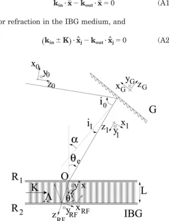
The polychromatic light guided by the fiber (Fig. 1) is collimated by an objective into a Gaussian beam. It is dispersed by the diffraction grating G so that the incide¸nce angle on the intracavity Bragg grating de-pends on the wavelength. The particular construction of the IBG [25,28] with its grating fringes perpendic-ular to the mirrors of the asymmetric cavity 共R1 ⫽ 1 and R2⯝ 1) implies that only the light arriving at the Bragg angle is efficiently diffracted (the cavity being tuned to this incidence), counterpropagating the incident beam. The light arriving at a different incidence is reflected by the IBG. The diffracted beam can easily be retrieved using a beam splitter or a circulator [29]. In that way, the light corresponding to a particular wavelength is separated from the rest of the polychromatic beam. To switch from this wave-length to another, one can change the grating period so that the Bragg condition is fulfilled for the new wavelength, and the corresponding beam returns in counterpropagation. In practice, the IBG diffracts the light in a certain range of incidence, but only the light having exactly the Bragg incidence is returned in precise counterpropagation. The filter can be made more selective through spatial filtering [26,27]. This can be implemented, for instance, by the injection of the diffracted beam into a single-mode fiber (see Fig. 1).
Simple expressions of the selectivity␦ and tuning range⌬ of the filter can be obtained when the filter selectivity is limited by the final spatial filtering (as is the case of the experiments described in [26,27] for instance). Since the diffraction grating period is much smaller than the acoustic period ⌳, the wavelength dispersion of the IBG grating can be neglected com-pared with that of the diffraction grating, and the spectral bandwidth is
␦ ⫽ 兾2NR, (1) where NRis the number of grooves of the diffraction grating that are illuminated by the beam. NRdepends
on the ratio of the beam diameter to the diffraction grating period. The tuning range is
⌬ ⫽2 ⌬⌳⌳ NNB R
, (2)
where⌬⌳ is the Bragg grating tuning range, deter-mined by the AO device, and NB is the number of periods of the IBG illuminated by the beam. It can be noted that the diameter of the beam incident on the IBG depends on the dispersion of the diffraction grat-ing. The Fabry–Perot etalon is adjusted for a maxi-mum transmission at the desired wavelength to provide a great enhancement of the filter efficiency, but it does not influence the tuning range of the filter. The number of resolvable wavelengths is then
N⫽⌬⌳
⌳ NB. (3)
Since its spectral bandwidth essentially depends on
NRand the number of resolvable lines depends on NB it is easy to optimize them separately.
These simple equations give a good idea of the filter selectivity that can be reached. Nevertheless, to ob-tain information about the diffraction efficiency and also an accurate value of the transmission band-width, it is necessary to develop a numerical simula-tion taking into account all the aspects of the light propagation in the device.
3. Model
The aim of this model is to calculate the transmission
Pout兾Pinof the filter as a function of the wavelength of the incoming light. For that purpose, we take into ac-count the effect of each element on the propagation of the light beam. Part of this task has been carried out in a previous study, where a calculation of the diffraction of Gaussian beams in the IBG has been developed [28]. In this calculation, the Gaussian beam is expanded in a plane wave basis. An analytical expression of the diffraction efficiency of each plane wave is obtained through a coupled wave analysis [30], and the bound-ary conditions are imposed by the cavity. Those effi-ciencies are then numerically summed to provide the diffraction efficiency of the complete beam.
In the present work, the beam traveling in the filter is also expanded in plane waves. Note that all optical elements on the beam path are considered large com-pared with the beam waist. The deviation of each wave by the diffraction grating is considered to de-termine analytically the amplitude of the incident waves on the IBG surface (see Subsection 3.A and Appendix A). The amplitude of the diffracted re-flected waves in the reference frame 共0, x, y, z兲 of the IBG is derived from the IBG diffraction calcula-tion. Taking into account the deviation attributable to the diffraction grating on the way back (Subsection 3.B and Appendix B), an analytical value of the inci-dent field on the spatial filter is obtained. A
ical sum is then carried out to determine the power of the light going through the spatial filter.
A. Way to the Intracavity Bragg Gratings
In our filter, the incoming beam is collimated from a single-mode fiber. The fiber mode of radius r is colli-mated by an objective of focal length f into a beam of waist w0 ⫽ f兾r (Fig. 2). In the reference frame of the objective 0共O0, x0, y0, z0兲, the complex electric field of the incident light is described as a plane wave of wave vector k0共0兲共0, 0, k兲 multiplied by an ampli-tude R0共x0, y0兲 that defines the Gaussian shape of the beam. The amplitude R˜共␦k0 x0,␦ky0兲 of a Fourier
com-ponent of R0共x0, y0兲 is then R0 ˜共␦k x0, ␦ky0, z0兲⫽
冑
2Pinw0 2 c exp冋
⫺ w0 2 2共
␦kx0 2⫹ ␦k y0 2兲
册
, (4)where Pinis the power incident onto the filter. Note that this expression is valid because we are inter-ested in the propagation of a low-divergence beam on a small length.
The input beam is thus expanded into plane waves whose wave vectors can be written as the wave vector of the central plane wave k0共0兲 to which a deviation
␦k0 ⫽ 共␦kx0,␦ky0,␦kz0兲 is added. The changes
under-gone by the plane wave components at each element of the filter are explained in Appendix A.
It is therefore possible to derive the Fourier com-ponent amplitude R˜共␦kI x,␦ky兲 of the beam incident onto the IBG, expressed in the frame:
RI ˜共␦kx, ␦ky兲 ⫽
冑
2PIw02 cn0 exp冋
⫺w0 2 2冉
⫺ cos共i1兲 共cos共i0兲cos共e兲兲 ⫻ ␦kx冊
2 ⫹ ␦ky2册
. (5) Reference [28] is used to derive the Fourier com-ponents amplitudes of the forward and backward read and diffracted beams propagating in the IBG. The Fourier components amplitudes of the reflected– diffracted beam coming out of the IBG S˜DR共␦kx,␦ky, 0兲 can then be computed and used for the analysis of the propagation to the output of the filter.B. Way Back from the Intracavity Bragg Gratings
The amplitude S˜0共k3x0, k3y0兲 of the Fourier component
of the field entering the spatial filter is given by
SDR
˜共␦kx,␦ky兲 provided the path of the reflected– diffracted beam from the IBG to the output spatial filter is taken into account. This is detailed in Appen-dix B.
The total power Poutcoming out of the filter that can be coupled to the fundamental mode of a fiber is given by [31] Pout⫽ c 2
冨
冕冕
⫺⬁ ⫹⬁ dxFdyFEF*共xF, yF兲EM共xF, yF兲冨
2冕冕
⫺⬁ ⫹⬁ dxFdyFⱍ
EM共xF, yF兲ⱍ
2 , (6)where the amplitude of the actual field at the surface of the fiber (the filter output) EF共xF, yF兲 is projected on the Gaussian modal field amplitude of this fiber
EM共xF, yF兲. It can be noted that the Gaussian mode is normalized
冕冕
⫺⬁ ⫹⬁dxFdyF
ⱍ
EM共xF, yF兲ⱍ
2⫽ 1. (7)The objective of the spatial filter performing a Fou-rier transform on the field, in the paraxial approxi-mation used in this analysis, the power Poutcan also be obtained by summing on the Fourier transform of the field incident on the objective:
Pout⫽ c 2
冨
冕冕
⫺⬁ ⫹⬁ dk3x0dk3y0S ˜ 0共
k3x0, k3y0兲
M ˜共
k3x0, k3y0兲
冨
2 , (8)where S˜0共k3x0, k3y0兲 and M˜共k3x0, k3y0兲 ⫽ w0兾
冑
exp关⫺共w02兾2兲共k3x0
2 ⫹ k 3y0
2兲兴 are the Fourier transforms of
EF*共xF, yF兲 and EM共xF, yF兲 respectively. Note that for a beam coming out of the filter (wave vector k3, see Fig.
3), as EF*共xF, yF兲 and EM共xF, yF兲 are the fields in the image focal plane of the objective used for the spatial filtering at the output, S˜0共k3x0, k3y0兲 and M˜共k3x0, k3y0兲 are
the Fourier transforms of these fields in the object focal plane. Moreover, we use the fact that, in the paraxial approximation, S˜0共k3x0, k3y0兲 and M˜共k3x0, k3y0兲
also represent the field distributions in the lens plane
Fig. 2. Collimation of the beam from the fiber.
within a constant phase change. We found out that it was easier to perform the numerical sum in theᏮ3 basis (see Appendix B). After the adequate vari-able change, the power coupled into the fiber is then given by Pout⫽ c 2
冨
冕冕
⫺⬁ ⫹⬁冉
cos共i2兲cos共i3⫺ i0兲 cos共i3兲cos共e⬘兲 d␦kxd␦kyS˜DR共␦kx, ␦ky, 0兲冊
⫻ M
冉
coscos共i2兲cos共i3⫺ i0兲共i3兲cos共e⬘兲 ␦kx⫺ k sin共i3⫺ i0兲, ␦ky, 0
冊
冨
2
. (9)
When the spatial filtering is performed by a hole, as in the experiments described in [27] Eq. (9) is no longer valid. The transmitted power is then
P⫽ c
2
冕冕
xF2⫹yF2⬍r2dxFdyF
ⱍ
EF共xF, yF, 0兲ⱍ
2. (10)In this case, the transmitted power is calculated from the integral over the plane of the hole 共xF2 ⫹ yF2 ⬍ r2兲 of the intensities of E
F共xF, yF, 0兲. This condition can also be expressed in the Fourier space, either by using the Parseval theorem or by noting that only the plane waves converging on the points共xF, yF, 0兲 sat-isfying xF
2⫹ y F
2⬍ r2
go through the hole. This last inequality is equivalent to
冉
k3x0f k冊
2 ⫹冉
k3y0f k冊
2 ⬍ r2and it is therefore convenient to use polar coordi-nates in the Fourier space: k3x0 ⫽ cos and k3y0
⫽ sin . The light power that is transmitted is given by the sum of the squared modulus of ampli-tudes of the plane waves fulfilling the latter condi-tion. The power injected into the hole is therefore
P⫽ c 2
冕
0 2 d冕
0 rk兾f dⱍ
S˜0共 cos , sin , 0兲ⱍ
2 , (11) or P⫽ c 2冕
0 2 d冕
0 rk兾f dⱍ
S˜DR共␦kx, ␦ky, 0兲ⱍ
2 , (12) with ␦kx⫽冉
cos ⫺冉
2 0冊
sin共i3⫺ i0兲冊
cose⬘cos i3 cos共i3⫺ i0兲cos i2,
(13)
␦ky⫽ sin . (14)
The simulation of the filter’s response is then com-plete, and its results can be compared with the ex-periments.
4. Numerical Analysis of Experimental Data at 760 nm In the experiments described in [27], a commercial AO cell, which is actually a modulator, is used with a mirror at its back. As the acoustic velocity in this 3 mm wide TeO2 crystal is 4200 m兾s, it takes less than 1s 共3.10⫺3兾4200 ⫽ 0.7 ⫻ 10⫺7s兲 to change the acoustic frequency, in order to tune the filter to a new wavelength. This configuration is equivalent to an intracavity Bragg grating with a null reflectivity for the front mirror. It is thus not angularly very selec-tive, but the desired wavelength can be selected with a good resolution through spatial filtering. The re-turning light is extracted with a beam splitter and injected, thanks to a lens, into a pinhole, which achieves the spatial filtering. The light source is a tunable Ti–Sa laser operated in the single-mode re-gime, using a fixed intracavity Fabry–Perot etalon. As a consequence, the wavelength is not tuned con-tinuously but jumps discretely from one mode of the etalon to the other with a wavelength step of 0.43 nm. To obtain a Gaussian beam, the laser light is injected into a single-mode fiber and collimated in a 0.5 mm waist beam. The diffraction grating has a 555 nm period and is used in the Littman configuration. The
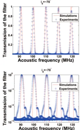
Fig. 4. Transmission of the filter as a function of the acoustic frequency for five wavelengths at⬃760 nm with a space of 0.43 nm 共225 GHz exactly). Linear scale on the upper curve and semiloga-rithmic scale on the lower one.
beam is incident at 70° on the diffraction grating. For five different Ti–Sa laser wavelengths at approxi-mately 760 nm, the transmission of the filter is mea-sured as a function of the acoustic frequency, the latter being directly linked to the AO grating period. The corresponding spectra are shown in Fig. 4. The acoustic FWHM is 1.6 MHz, which gives the possibil-ity to resolve 30 different optical frequencies within the 50 MHz tuning range of the AO modulator used in our experiment. The linear scale shows the good uniformity of the filter transmission; the selected wavelength is always at Bragg incidence and experi-ences the same diffraction efficiency, in the whole tuning range, which would not be the case with other filtering techniques using AO devices [24]. On the logarithmic scale, one can see that the sidelobes are down to 20 dB below the maxima, which makes them quite harmless for most applications. They are due to the limited aperture of the AO cell, causing diffrac-tion of the beam, as it is widened after the diffracdiffrac-tion on the grating. The demonstrated optical tuning range is 2.2 nm, centered on 760 nm.
In Fig. 4, the experimental data can be compared with the simulations using precisely the experimen-tal parameters. The curves are normalized because the losses on the diffraction grating and the beam splitter are not taken into account. Anyway, these losses could be made very small by using a circulator
instead of the beam splitter as well as an adapted diffraction grating.
Moreover, although there is no adjustable param-eter, a very good agreement between experiments and simulation is obtained on the position and width of the peaks, which provides a validation of our nu-merical simulation. It is then possible to calculate the performances of optimized filters.
5. Optimized Filters at 1550 nm
The AO cell Bragg grating used in the experiments of [27] allowed us to test the feasibility of the filter and to validate the simulation. Nevertheless, no element of the device was specially designed for this application. We now present the calculated performances that could be reached with commercially available Bragg and diffraction gratings specifically chosen to optimize the tunable filter for DWDM communication. The impact of the wavelength range at approximately 1.55m is taken into account in the equation, but the main change would come from the choice of an opti-mized AO cell and a suitable diffraction grating pe-riod, as explained hereafter.
The main limitation of the experimental filter pre-sented in Section 4 is the width of the Bragg grating or more precisely the number NR of illuminated pe-riods of the AO cell, as it is directly bound to the number of channels in the tuning range of the filter
Fig. 5. Transmission spectrum of the filter at approximately 1550 nm with a 17 mm wide acousto-optic cell at an acoustic frequency of 170 MHz (left) and 290 MHz (right). The upper plots have a linear scale and the lower ones have a semilogarithmic scale.
[see Eq. (3)]. Commercial AO deflectors can be found with a width of 17 mm (to be compared with the 3 mm width of our modulator). Moreover, their acous-tic tuning range is 120 MHz instead of 50 MHz for the modulator. It is interesting to evaluate how these characteristics can improve the filter performances.
With the help of Eq. (1), a configuration is chosen that generates transmission peak widths of 0.2 nm to match the DWDM communications requirements. We choose a beam waist w0of 5 mm and an incidence angle i0⫽ ⫺40° on a diffraction grating with a period
a ⫽ 4 m. The angle between the Bragg and the
diffraction grating is chosen so that the tuning range spreads at approximately 1.55m.
Figure 5 shows the transmission peaks for acoustic frequencies of 170 and 290 MHz that correspond to the limits of the tuning range spreading from 1503, 6 nm to 1599, 6 nm共⌬ ⫽ 96 nm兲. The linear scale of the upper plots is convenient to see the chan-nel bandwidth whereas the semilogarithmic scale of the lower plots is useful to evaluate the cross-talk performances. The FWHM of the peaks are ␦ ⫽ 0, 19 nm共24 GHz兲 for F ⫽ 170 MHz and ␦ ⫽ 0, 21 nm共27 GHz兲 for F ⫽ 290 MHz. The number of distinguishable wavelengths is thus N ⫽ 480. The widths of the peaks at⫺25 dB are 0, 55 nm 共70 GHz兲 and 0, 61 nm共76 GHz兲. The number of telecommuni-cation channels with an overlap of ⫺25 dB is 165, with a perfect transmission uniformity. The tuning speed would be 4s in this 17 mm wide crystal. It can be concluded that this device is most interesting for DWDM communications.
Note that the add– drop function could be achieved with an angularly very selective IBG, obtained with a very high finesse Fabry–Perot resonator. As shown in Fig. 1 of [27] the reflected light would also be re-trieved using another diffraction grating set symmet-rically to the first one, to redirect all remaining wavelengths toward the same direction. The device could also be used as the external cavity of a tun-able laser, especially in the case of a fiber laser where the reinjection into the fiber automatically achieves the necessary spatial filtering.
6. Conclusion
A high performance filtering technique associating a diffraction grating to an intracavity Bragg grating has been demonstrated. The developed simulation is in good agreement with the experimental results and is used to design optimized devices. A simple setup without a cavity and using commercially available elements could have a transmission bandwidth of 0.2 nm with a tuning range of 96 nm, which makes it suitable for a DWDM application. The adaptability of this filtering technique is very wide. The selectivity and the tuning range can be chosen just by turning or changing the diffraction grating. The only limitation is the number of distinguishable frequencies, which is given by the characteristics of the Bragg grating (es-pecially its width). Add– drop functions, bandpass fil-ter and tunable lasers could also be achieved with a more sophisticated intracavity Bragg grating, which
can be designed using the theoretical analysis given herebefore.
Appendix A: Way to the Intracavity Bragg Gratings This is the detailed analysis of the propagation of the plane wave components of the Gaussian beam from the input of the filter to the IBG. The relation be-tween the wave vectors deviation from the central propagation direction ␦k0 ⫽ 共␦kx0,␦ky0兲 and ␦k ⫽
共␦kx,␦ky兲 of the plane wave components at the injec-tion objective and the IBG, respectively, is deter-mined by the beam propagation from the output of the fiber to the IBG. It then depends on the incidence angles i0 and e of the central wave vector on the traditional and intracavity gratings, respectively.e depends on the angle between the gratings’ normal␣ via the relatione⫽ i0⫺ ␣. These angles are repre-sented in Fig. 6. For each part of the path, the wave vectors can be expressed in a basis whose z axis is in the direction of the central wave vector. The relations between the directions of a given plane wave before and after an element are easily determined by writ-ing their wave vectors in the basis of the element (all bases are represented in Figs. 6 and 7). As no direc-tion change occurs along the y axis, the deviadirec-tion␦ky is constant during the whole process and we only need to relate the x deviation␦kxito␦kxi⫹1. This is done
by applying the conservation of the wave-vector pro-jection on the boundary plane, taking its periodicity into account. The incoming wave vector kinis related
to the outcoming one koutin the following way:
kin· xˆ⫺ kout· xˆ⫽ 0 (A1)
for refraction in the IBG medium, and
共kin⫾ K兲· xˆj⫺ kout· xˆj⫽ 0 (A2)
Fig. 6. (Color online) Angles defining the path of the central plane wave from the fiber to the IBG.
for diffraction by a grating with a wavevector K par-allel to xˆj.
Table 1 shows the relations between the incidence angles of the central wave and also between the de-viations of a given off-axis plane wave at each inter-face. KGis the wave vector of the grating G.
A deviation ␦kx0 with respect to the central wave
vector at the fiber exit leads to a deviation␦kxRFat the surface of the IBG, and a relation between those de-viations can be obtained by using Table 1. Expressed in the reference frame共O, x, y, z兲 the deviation be-comes␦kx⫽ ␦kxRFcos共兲. We have thus the relation
␦kx0⫽ ⫺
cos共i1兲 cos共i0兲cos共e兲␦kx
,
and␦ky0⫽ ␦ky.
Appendix B: Way Back from the Intracavity Bragg Gratings
This is a detailed analysis of the propagation of the plane wave components of the Gaussian beam from the IBG to the output of the filter. Therefore we need to express the central wave vectors ki and the wave
vectors of the plane wave components␦kiof the beam
at every stage of the path so that k3 and ␦k3
⫽ 共␦k3x0,␦k3y0兲 at the output of the filter in the
refer-ence frame of the output objective can be related to k and␦k ⫽ 共␦kx,␦ky兲 in the IBG.
As in the case of the forward propagation in the filter, this relation depends on the incidence angles and2and emergence anglese⬘ and 3of the central wave vector on G and IBG (see Fig. 7). Table 2 shows the relations between the incidence angles of the cen-tral wave and also between the deviations of a given off-axis plane wave at each stage. These relations are obtained by using Eqs. (A1) and (A2) for the way to the output of the filter. From Table 2 and using ␦kxSRcos⬘ ⫽ ␦kxin order to take the tilt of the IBG into account, we get
␦kx3⫽ ⫺
cos共i2兲
cos共e⬘兲cos共i3兲␦kx
, (B1)
in the frame Ꮾ3共O3, x3, y3, z3兲 corresponding to the beam at the entrance of the spatial filter. In the focal plane of the objective 共O0, x0, y0兲 the central wave vector of the incoming beam k3共0兲is at an angle i3 ⫺
i0 ⫹ to the original beam. Only a monochromatic beam having exactly the selected wavelength is in precise contrapropagation and thus at an angle of. The final step is to change the basis fromᏮ3to the basis of the objectiveᏮ0through a ⫹ i3⫺ i0rotation about y3. Using the equations of Tables 1 and 2, it is then possible to express the vector k3共k3x0, k3y0, k3z0兲 as
a function of the variables␦kxand␦ky, which are used in the IBG diffraction model conputation. We thus have
kx3⫽
cos共i2兲 cos共i3兲cos共e⬘兲 ␦
kxcos共i3⫺ i0兲 ⫹ k sin共i3⫺ i0兲. (B2)
References
1. D. Sadot and E. Boimovich, “Tunable optical filters for dense wdm networks,” IEEE Commun. Mag. 36, 50 –55 (1998). 2. M. Fukutoku, K. Oda, and H. Toba,
“Wavelength-division-multiplexing add兾drop multiplexer employing a novel polari-sation independent acousto-optic tunable filter,” Electron. Lett. 29, 905–907 (1993).
3. Y. W. Song, Z. Pan, D. Starodubov, V. Grubsky, E. Salik, S. A. Havstad, Y. Xie, A. E. Willner, and J. Feinberg, “All-fiber wdm optical crossconnect using ultrastrong widely tunable fbgs,” IEEE Photon. Technol. Lett. 13, 1103–1105 (2001).
4. J. E. Ford, V. A. Aksyuk, D. J. Bishop, and J. A. Walker, “Wavelength add drop switching using tilting micromirrors,” J Lightwave Technol. 17, 904 –911 (1999).
5. D. Marom, D. Neilsont, and D. Greywall, “Wavelength-selective 1⫻ 4 switch for 128 wdm channels at 50 ghz spacing,” in Optical Fiber Communication Conference and Exhibit, 2002 (OFC, 2002), pp. FB7-1–FB7-3.
Fig. 7. Angles defining the path of the central plane wave from the IBG back to the fiber.
Table 1. Relations Between Wave Vectors Before the Intracavity Bragg Gratings
Diffraction Refraction Central
wave i1⫽ ⫺arcsin
冉
sin共i0兲 ⫾KG k
冊
⫽ arcsin冉
sin共e兲 n冊
Off-axis plane wave ␦kx1⫽ ⫺ cos共i0兲 cos共i1兲␦k x0 ␦kxRF⫽ cos共e兲 cos共兲 ␦kx1Table 2. Relations Between Wave Vectors After the Intracavity Bragg Gratings
Refraction Diffraction Central
wave
e⬘ ⫽ arcsin共n sin共⬘兲兲 i
3⫽ ⫺arcsin
冉
sin共i2兲 ⫾KG k
冊
Off-axis plane wave ␦kx2⫽ cos共⬘兲 cos共e⬘兲␦k xSB ␦kx3⫽ ⫺ cos共i2兲 cos共i3兲␦k x26. W. Duncan, T. Bartlett, B. Lee, D. Powell, P. Rancuret, and B. Sawyers, “Dynamic optical filtering in dwdm systems using the dmd,” Solid-State Electron. 46, 1583–1585 (2002). 7. B. Heffner, D. Smith, I. Baran, A. YI-Yan, and K. Cheung,
“Integrated-optic acoustically tunable infrared optical filter,” Electron. Lett. 24, 1562–1563 (1988).
8. K. W. Cheung, D. A. Smith, J. E. Baran, and B. L. Heffner, “Multiple channel operation of an integrated acousto-optic,” Electron. Lett. 25, 375–376 (1989).
9. M. S. Borella, “Optical components for wdm lightwave net-works,” Proc. IEEE 85, 1274 –1307 (1997).
10. D. Ostling and H. Engan, “Spectral flattening by an all-fiber acousto-optic tunable filter,” in Proceeding of Ultrasonics
Sym-posium (Seattle, 1995), Vol. 2, pp. 837– 840.
11. H. S. Kim, S. H. Yun, I. K. Kwang, and B. Y. Kim, “Low-loss all-fiber acousto-optic tunable filter,” Opt. Lett. 22, 1476 –1478 (1997).
12. S. H. Yun, D. J. Richardson, D. O. Culverhouse, and T. A. Birks, “All-fiber acoustooptic filter with low-polarization sen-sitivity and no frequency shift,” IEEE Photon. Technol. Lett. 9, 461– 463 (1997).
13. D. S. Starodubov, V. Grubsky, and J. Feinberg, “All-fiber band-pass filter with adjustable transmission using cladding-mode coupling,” IEEE Photon. Technol. Lett. 10, 1590 –1592 (1998). 14. A. Spisser, R. Ledantec, C. Seassal, J. L. Leclercq, T. Benyat-tou, D. Rondi, R. Blondeau, G. Guillot, and P. Viktorovitch, “Highly selective and widely tunable 1.55m inp兾air-gap mi-cromachined Fabry–Perot filter for optical communications,” IEEE Photon. Technol. Lett. 10, 1259 –1261 (1998).
15. R. Le Dantec, T. Benyattou, G. Guillot, A. Spisser, J. L. Leclercq, P. Viktorovitch, D. Rondi, and R. Blondeau, “Tunable microcavity based on inp air Bragg mirrors,” IEEE J. Sel. Top. Quantum Electron. 5, 111–114 (1999).
16. P. Tayebati, P. D. Wang, D. Vakhshoori, and R. N. Sacks, “Widely tunable Fabry–Perot filter using ga(al)as alox deform-able mirrors,” IEEE Photon. Technol. Lett. 10, 394 –396 (1998). 17. J. Peerlings, A. Dehe, A. Vogt, M. Tilsch, C. Hebeler, F. J. Langenhan, P. Meissner, and H. L. Hartnagel, “Long resonator micromachined tunable gaas alas Fabry–Perot filter,” IEEE Photon. Technol. Lett. 9, 1235–1237 (1997).
18. J. Daleiden, V. Rangelov, S. Inner, E. Romer, M. Strassner, C. Prott, A. Tarraf, and H. Hillmer, “Record tuning range of inp-based multiple air-gap moems filter,” Electron. Lett. 38, 1270 –1271 (2002).
19. M. Strassner, J. C. Esnault, L. Leroy, J.-L. Leclercq, M.
Gar-rigues, and I. Sagnes, “Fabrication of ultrathin and highly flexible inp-based membranes for micro-optoelectromechanical systems at 1.55m,” IEEE Photon. Technol. Lett. 17, 804–806 (2005).
20. J. Berger, F. Ilkov, D. King, A. Tselikov, and D. Anthon, “Widely tunable, narrow optical bandpass Gaussian filter us-ing a silicon microactuator,” In Optical Fiber Communication
Conference (OFC), Postconference Digest (IEEE, 2003), Vol. 86,
pp. 252–253.
21. G. Wilson, C. J. Chen, P. Gooding, and J. E. Ford “Spectral filter with independently variable center wavelength and bandwidth,” in 30th ECOC Proceedings, Stockholm, Sweden, September 2004.
22. W. Huang, R. R. A. Syms, J. Stagg, and A. Lohmann, “Preci-sion mems flexure mount for a Littman tunable external cavity laser,” IEE Proc.: Sci. Meas. Technol. 151, 67–75 (2004). 23. A. A. Tarasov, H. Chu, and Y. M. Jhon,
“Polarization-independent acousto-optically tuned spectral filter with fre-quency shift compensation,” IEEE Photon. Technol. Lett. 14, 944 –946 (2002).
24. E. G. Paek, J. Y. Choe, and T. K. Oh, “Transverse grating-assisted narrow-bandwidth acousto-optic tunable filter,” Opt. Lett. 23, 1322–1324 (1998).
25. L. Menez, I. Zaquine, A. Maruani, and R. Frey, “Intracavity Bragg gratings,” J. Opt. Soc. Am. B 16, 1849 –1855 (1999). 26. D. Bitauld, C. Martins, I. Zaquine, A. Maruani, R. Frey, R.
Chevallier, and L. Dupont, “Tunable optical filtering with an intracavity bragg grating associated to a standard grating,” in
Conference on Lasers and Electro-Optics, 2004 (CLEO) (IEEE,
2004), Vol. 2.
27. D. Bitauld, I. Zaquine, A. Maruani, and R. Frey, “Grating-assisted uniform response high resolution tunable optical fil-tering using a grating-assisted acousto-optic device,” Opt. Express 13, 6438 – 6444 (2005).
28. D. Bitauld, L. Menez, I. Zaquine, A. Maruani, and R. Frey, “Diffraction of Gaussian beams on intracavity Bragg gratings,” J. Opt. Soc. Am. B 22, 1153–1160 (2005).
29. Y. Fujii, “High-isolation polarization-independent optical cir-culator coupled with single-mode fibers,” J. Lightwave Tech-nol. 19, 1238 –1243 (1991).
30. H. Kogelnik, “Coupled wave theory for thick hologram grat-ings,” Bell. Syst. Tech. J. 48, 2909 –2947 (1969).
31. S. Vatoux, Y. Combemale, A. Enard, J. Arnoux, and M. Papuchon, L’optique Guide Monomode (Masson, 1985), pp. 663–710.