Recognition of Facial Expressions with Autoencoders and Convolutional-Nets

(1)

Université de Montréal

Recognition of Facial Expressions with Autoencoders and

Convolutional-Nets

par Hani Almousli

Département d’informatique et de recherche opérationnelle Faculté des arts et des sciences

Mémoire présenté à la Faculté des études supérieures et postdoctorales en vue de l’obtention du grade de Maître ès sciences (M.Sc.)

en informatique

2013

(2)

Résumé

Les humains communiquent via différents types de canaux: les mots, la voix, les gestes du corps, des émotions, etc. Pour cette raison, un ordinateur doit percevoir ces divers canaux de communication pour pouvoir interagir intelligemment avec les humains, par exemple en faisant usage de microphones et de webcams.

Dans cette thèse, nous nous intéressons à déterminer les émotions humaines à partir d’images ou de vidéo de visages afin d’ensuite utiliser ces informations dans différents domaines d’applications. Ce mémoire débute par une brève introduction à l'apprentissage machine en s’attardant aux modèles et algorithmes que nous avons utilisés tels que les perceptrons multicouches, réseaux de neurones à convolution et autoencodeurs. Elle présente ensuite les résultats de l'application de ces modèles sur plusieurs ensembles de données d'expressions et émotions faciales.

Nous nous concentrons sur l'étude des différents types d’autoencodeurs (autoencodeur débruitant, autoencodeur contractant, etc) afin de révéler certaines de leurs limitations, comme la possibilité d'obtenir de la coadaptation entre les filtres ou encore d’obtenir une courbe spectrale trop lisse, et étudions de nouvelles idées pour répondre à ces problèmes. Nous proposons également une nouvelle approche pour surmonter une limite des autoencodeurs traditionnellement entrainés de façon purement non-supervisée, c'est-à-dire sans utiliser aucune connaissance de la tâche que nous voulons finalement résoudre (comme la prévision des étiquettes de classe) en développant un nouveau critère d'apprentissage semi-supervisé qui exploite un faible nombre de données étiquetées en combinaison avec une grande quantité de données non-étiquetées afin d'apprendre une représentation adaptée à la tâche de classification, et d'obtenir une meilleure performance de classification. Finalement, nous décrivons le fonctionnement général de notre système de détection d'émotions et proposons de nouvelles idées pouvant mener à de futurs travaux.

Mots-clés : Intelligence artificielle, apprentissage machine, réseaux de neurones,

(3)

Abstract

Humans communicate via different types of channels: words, voice, body gesture, emotions …etc. For this reason, implementing these channels in computers is inevitable to make them interact intelligently with humans. Using a webcam and a microphone, computers should figure out what we want to tell from our voice, gesture and face emotions.

In this thesis we are interested in figuring human emotions from their images or video in order to use that later in different applications. The thesis starts by giving an introduction to machine learning and some of the models and algorithms we used like multilayer perceptron, convolutional neural networks, autoencoders and finally report the results of applying these models on several facial emotion expression datasets.

We moreover concentrate on studying different kinds of autoencoders (Denoising Autoencoder , Contractive Autoencoder, …etc.) and identify some limitations like the possibility of obtaining filters co-adaptation and undesirably smooth spectral curve and we investigate new ideas to address these problems. We also overcome the limitations of training autoencoders in a purely unsupervised manner, i.e. without using any knowledge of task we ultimately want to solve (such as predicting class labels) and develop a new semi-supervised training criterion which exploits the knowledge of the few labeled data to train the autoencoder together with a large amount of unlabeled data in order to learn a representation better suited for the classification task, and obtain better classification performance. Finally, we describe the general pipeline for our emotion detection system and suggest new ideas for future work.

Keywords: Artificial Intelligence, machine learning, neural nets, autoencoders, unsupervised

(4)

List of Tables

Table 1: Dataset used to build Toronto Faces Dataset (TFD) with their accessibility [36]. ... 20

Table 2: The effect of applying maximum weight on classification for both TFD and MNIST using dropout ... 35

Table 3: The effect of varying batch size on TFD classification. ... 37

Table 4: Comparision between DAE and SSDAE classification on TFD, MNIST and CIFAR100. Numbers in paranthesis are standard deviation of accuracy on the TFD splits. ... 45

Table 5: Conv net pre-trained using SSDAE on TFD folds. ... 47

Table 6: ConvNet classification result on TFD ... 48

Table 7: ConvNet classification result on TFD using weight decay. ... 49

Table 8: ConvNet classification result on TFD using sigmoid output units instead of softmax ... 49

Table 9: ConvNet classification result on TFD using rectifier unit. ... 51

Table 10: ConvNet classification on TFD with rectifier varying the drop out probability and the number of feature maps... 52

(7)

List of Figures

Figure 1: A multi-layer perceptron with one hidden layer ... 9

Figure 2: LeNet CNN [27] ... 13

Figure 3: One feature map in CNN with weight sharing [27] ... 14

Figure 4: SVM hyper-plane seprating two classes [30]. ... 15

Figure 5: Visualization of how DAE works and its connection to manifold learning [33]. ... 17

Figure 6: Pre-processed examples from TFD [36]. ... 20

Figure 7: Average spectrum of the encoder's Jacobian for the CIFAR-bw dataset [35]. DAE-g, DAE-b corresponds to Gaussian and binomial corrupted DAE respectively. ... 24

Figure 8: Ideal Spectral Curve ... 25

Figure 9: Some filters learned by a DAE on TFD ... 31

Figure 10: DAE filters with small weights initialization ... 32

Figure 11: Effect of maximum weight on TFD using dropout. (a) small weight magnitude (b) bigger weigh magnitude ... 34

Figure 12: The effect of maximum weight with Dropout on MNIST. (a) small weight magnitude (b) bigger weigh magnitude ... 35

Figure 13: Filters on TFD when the same dropout mask is used for the whole batch. (a): Batch size equal 20 (b): Batch size equal 10 ... 37

Figure 14: Monitoring different criteria during manifold AE training. ... 39

Figure 15: The mean and standard deviation of the hidden units activation. ... 40

Figure 16: The reconstruction of some MNIST digits and some of the learned filters ... 41

Figure 17: The spectral curve of the Jacobian on MNIST. ... 42

Figure 18: Pixels Importance for TFD and MNIST using Random Forests ... 44

Figure 19: Some MNIST filters trained using SSDAE and the reconstruction of some images. ... 46

Figure 20: An image with pixels importances showing how dark border patch is sampled more than the dotted border patch due to higher center value. ... 46

(8)

Figure 22: Plotting the relationship between the number of feature maps and the test accuracy on TFD using drop out and rectifiers. ... 53 Figure 23: Screenshots from the webcam live demo ... 59 Figure 24: Screenshots from the live demo showing happy emotion ... 60

(9)

List of Abbreviations

MSE: Mean Square Error MLP: Multi-Layer Perceptron

CNN : Convolutional Neural Network SVM: Support Vector Machine

IID: Independent and Identically Distributed MLL: Maximum Log Likelihood

AE: Autoencoder

DAE: Denoising Autoencoder CAE: Contractive Autoencoder SSAE: Semi Supervised Autoencoder

SSDAE: Semi Supervised Denoising Autoencoder SVD: Singular Value Decomposition

(10)

Notations

 is a column vector in such that  The target label

 An N * d matrix of the finite dataset that is sampled from an unknown distribution (true distribution)

 The training set (part of D)

 The validation set (part of D and has no intersection with )

 The test set (part of D and has no intersection with and )  The Euclidean norm of a vector is ‖ ‖ √ √∑

 The logistic sigmoid function is ( )  The hyperbolic tangent ( ) _{( )} ( )  The rectifier ( ) ( )

 The Frobenius norm of a matrix A (A values are real numbers) || || √∑∑ √ ( )

(11)

I have done my master in one of the worst time I have ever had in my life due to the war happening in my country, Syria. Anything I have done or going to do in my life will be dedicated first to my bleeding country, my family (Rashaad, Amal and Ali) and my friends. On the other hand, I would love to thank my supervisor Pascal Vincent, the professors and students in LISA lab for their help and support. I also thank NSERC and Ubisoft for their financial support of this research.

(12)

(13)

Introduction

Two channels have been distinguished in human interaction [1]. The first one transmits explicit messages (ex: spoken words) while the second transmits implicit messages. Mehrabian [2] indicated that the verbal part (words) of a message contributes only for a 7% of the effect of the message, the vocal part (voice information) contributes for 38% while facial expressions contributes for 55% of the effect of the spoken message. For this reason, to build a real Artificial Intelligence (AI), it is necessary that computers and robots use information from both channels by being accompanied with artificial mind that enables them to communicate with humans through exchanging not only logical information but also emotional one.

Recognizing the facial expression of humans attracted the attention of the computer vision community a long time ago [3] [4]. On the other hand, human emotion recognition was studied in psychology [5] [6]. It is true that this problem can be considered as one of the hard tasks we wish our computers to solve. Its difficulty comes from its relation to psychology. To make it clearer, imagine you have an image for a person and you ask different people about this person’s emotion whether he is happy, sad, disgust, tired, humiliated, etc. It is not rare to find people disagreeing on the expressed emotion unless the picture is very obvious. This begs the question: given this task is hard and ambiguous for humans, how can we bring machines to perform it efficiently?

To tackle this problem, computer vision, signal processing and machine learning techniques have to be developed, while, at the same time, consolidating psychological and linguistic analyses of emotion. For example, Ekman and Friesen developed a measurement system for facial expression [7]. Their system is known as the Facial Action Coding System (FACS). It was developed based on a discrete emotions theoretical perspective and is designed to measure specific facial muscle movements. In many cases, people from psychology are the best to label human faces with the correct emotion, and then people from other disciplines try to build models according to this information.

(14)

This thesis focuses on predicting human emotion from facial expression images. We will have some labeled data and lots of un-labeled images. The task is to build a system to figure out person’s emotions from their images. Such system can later be used in many applications. For example, it can be used in future computer games to make them more interactive like changing the game flow depending on the player’s emotion. Currently, Microsoft Xbox and Sony PlayStation consoles are equipped with Kinect and PS move, respectively, which both have a motion capture system that allows the usage of body gestures in games. So it is natural to exploit facial expressions analysis in the near future by simply using a webcam and appropriate software.

The thesis core is divided logically into two main sections. The first section is research oriented one which studies some of the autoencoders limitations and introduces new solutions for these problems with experiments. The second one talks about human emotion detection software, the algorithms, models and experiments used to build that system.

The thesis is organized as follows:

 Part Ι: Machine Learning Background and Literature

Chapter 1: gives a short introduction to machine learning basic principles and concepts which are necessary to understand the thesis.

Chapter 2: describes the machine learning models that were studied and implemented for both research reasons and to build the human emotion recognition software.

Chapter 3: describes some of the human emotion dataset used to do experiments and train models on.

 Part ΙΙ: Novel Ideas and Experiments

Chapter 4: concentrates on limitations with the current autoencoder approaches and proposes new solutions to overcome these problems.

Chapter 5: lists part of the experiments done to improve state of the art autoencoders and to experiment models studied in chapter Chapter 4:

Chapter 6: Experiments on convolutional nets to build models that can be used in the human emotion detection software.

(15)

Finally, the appendix describes the human emotion detection live demo with some screen shots.

(16)

(17)

Chapter 1: Brief Introduction to Machine Learning

1.1 Machine Learning Definition

A nice definition of machine learning is given in Kevin Murphy’s book “A set of methods that can automatically detect patterns in data and then use the uncovered patterns to predict future data, or to perform other kinds of decision making under uncertainty” [8]

Machine Learning is a branch of Artificial Intelligence which focuses on developing models to represent some of the characteristics of the world in order to make machines intelligent. In 1950 Alan Turing introduced an intelligence test in his paper Computing Machinery and Intelligence and he started with “Can machine think?” Machine Learning tries to imitate human brain in order to make machines act like humans in different fields like Vision, Natural Language …etc.

People working in machine learning start with the same assumption that physicists use to construct their field, we assumes that every natural data (images, text, speech …etc.) has a structure and we try to learn this structure in order to generalize for new unseen data. Mathematically speaking, it can be seen as a finite sample from an unknown natural distribution (typically considered a random vector variable, i.e. a vector of scalar random variable), and we try to model the underlying structure (joint distribution between these scalar random variables) from these samples.

1.2 Types of Learning

There are two main types of machine learning:

 Supervised Learning: learns a function which takes as an input from the training set _{ _}

{( )} where is the label and maps these

x’s such that ( ) i.e. f(x) attempts to predict the correct label t. Generally, the variables are assumed to be i.i.d. Supervised Learning is divided into two parts: Regression and Classification. In the former, the label to predict is a

(18)

continuous value while in the latter it is discrete. The main drawback of this type of learning is the necessity of having lots of labeled data, which is not always available, e.g. figuring out a face and non-face images.

 Unsupervised Learning: There are no labels so the dataset { } is given to the learning algorithm. The main task is probability density estimation. This type of learning is useful since we usually have lots of unlabeled data at our disposal, whereas labels are typically scarce. Examples of unsupervised learning are compression, clustering …etc.

1.3 Training VS. Generalization Error

During training, we estimate the performance of the function f using a cost function ( ) where ( ) belongs to the dataset D. This is called the empirical risk ̂. The general formula for ̂ is:

̂ ( ) ( ) ∑ ( ( )

)

The nature of L depends completely on the task we want to learn. An example of L:

 Regression: We want to learn a function f such that ( ) . The best choice is the mean square error (MSE):

( ( )) ( ( ) )

 Classification: The cost function should give the proportion of examples being assigned to the proper label by f. The convenient choice is the indicator function:

( ( )) _{( )}

 Density estimation: The goal is to maximize the occurrence of the input x by making

f(x) = p(x) as large as possible. A good choice is the log likelihood (MLL)

(19)

Since the training data is finite, the empirical risk computed with a finite dataset is a noisy estimator of the true expected risk we will obtain under the unknown true data distribution, which we can converge to it if we use an infinite amount of data from the distribution D. The true expected risk is also called generalization error, as it is a measure of how well the predictor f will perform, on average, on unseen examples. Training, using the empirical risk minimization principle, then consists of using a finite dataset to adapt a model’s parameters so that it achieves relatively low empirical risk on a finite training set. Yet good learning does not mean remembering examples by heart which can easily give zero error on a finite training set. The main goal is to have a robust model that achieves a low generalization error. The learned function should give a small error on different data that it is similar to the one it was trained on (assumed to be obtained from the same distribution) without having seen them during the training phase.

Practically, it is impossible to get an infinite amount of data from D so we use cross validation, i.e. evaluate our model on separate test data not used during training of its parameters, to insure that the model have a good ability to generalize. In its simplest form, cross validation means splitting the dataset into three folds, , , (typically

the last two splits have smaller size than the first). The function f is trained on the training split, we measure the empirical error on the validation split and we choose the function that has the minimum validation error, then we report the error on test data.

One of the successful ways of reducing the error on validation and test sets is to change the minimized cost function from being the empirical risk only by adding a regularization term. Regularization has a probabilistic interpretation of adding a prior knowledge to the model. The new cost function can be written as:

̂ ( )

̂( ) ( )

One of the possibilities of ( ) is the Euclidean norm of the model’s parameters which is called weight decay (check Chapter 6: for more information).

(20)

1.4 Hyper-Parameter Selection

Every machine learning algorithm has a set of hyper-parameters which are chosen before learning. Examples of hyper-parameters are the number of neurons in a neural net, the degree of the polynomial in regression, etc... Hyper-parameters are typically chosen using cross validation, i.e. searching and retaining the values that result in the best performance over a separate validation subset not used for training the model’s parameters (which are fitted to the training subset). There has recently been progress on how to more efficiently accomplish this task [9], [10].

1.5 Model Complexity

There is a relation between data complexity and optimal model capacity. The more complex the data is, the more complex the model should be. For example, data generated by a 3nd order polynomial cannot be approximated well with a linear model (under fitting). On the other hand, fitting data generated by a linear function plus simple noise by a high order polynomial gives a very bad generalization (over fitting). In addition more complex models (such as higher degree polynomials) will usually have more free parameters, which require more examples to estimate them correctly. A compromise should be achieved to choose model capacity by being neither too simple nor too complex.

(21)

Chapter 2: Machine Learning Algorithms

This section is going to describe some of the machine learning models and algorithms we worked on. Basically, we will talk about different types of neural nets and some of the practical tricks used to train these models.

2.1 Multi-Layer Perceptron (MLP)

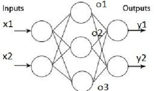
Figure 1: A multi-layer perceptron with one hidden layer

The Multi-Layer Perceptron (MLP) is a model used in supervised training which maps sets of input data into a set of appropriate output [11] [12] [13]. An MLP consists of multiple layers of nodes in a directed graph, with each layer fully connected to the next one. MLP can be considered as universal approximation for any type of function given enough capacity [14]. For this reason, the size of the network plays an important role in defining the complexity of the learned function [15]. The three main important things to know about MLP’s are forward propagation, backward propagation and how to train them correctly.

(22)

2.1.1 Forward propagation

Starting from the input, we calculate the output of each layer and feed it to the next layer until reaching the output layer. Generally, some nonlinearity like sigmoid or softmax is applied on the output of each layer (except the input). This step can be expressed in matrix form as:

( )

Finally a cost function, which we want to minimize, is calculated on the output of the MLP. Examples of these cost functions are

 Mean Square Error: ( ) ‖ ‖

 Binary Cross Entropy (output between 0 and 1): ( ) ∑ ( ) ( ) ( ) Where t is the actual target and is the predicted output.

The mean square error has a probabilistic interpretation that, given the input, the target value is Gaussian-distributed; while with the binary cross entropy it follows a Bernoulli distribution. The set of parameters that is to be learned (fitted to data) for such an MLP are: { }

2.1.2 Back propagation

This step is used to calculate the gradient of the cost function with respect to the network parameters ( : weights and biases) in order to update them in a way which minimizes the cost function over the training dataset [11]. The basic idea in this step is the chain rule.

The derivative of the cost function with respect to the output layer parameters is:

(23)

While the derivative of the cost with respect to the hidden layer parameters will be:

After calculating the gradients of the cost function with respect to the network parameters , we can update them using gradient descent:

The update rule can be applied on each example (stochastic gradient descent) or averaged on a mini-batch of several examples, or even on all training examples (batch gradient descent). What is called an “epoch” in what follows means one pass through all the examples of the training set.

2.1.3 Improving network performance

There are many practical tricks used to optimize the cost function and make the network generalizes better on unseen data [16] [17], to avoid learning training samples by heart (leading to over fitting and bad generalization performance). This section lists some important tricks used to train our models.

 Early Stopping: This trick is used to avoid over fitting. After each training epoch, the cost function is calculated on a validation data (never seen during training). The learning stops once the validation error starts increasing significantly from its reached minimum while the training error keeps going down.

 Weight decay: Used also to avoid over fitting by augmenting the cost function L(x) with regularization term ( ) 𝜆 ‖ ‖ where 𝜆 is a hyper-parameter. Either L1 or L2 norm are typically used. Each has an interpretation as a Bayesian prior over parameter values (respectively Gaussian and Laplacian).

 Adaptive learning rate with validation error: At the beginning of the training, we start with a big learning rate (as big as possible), and then, whenever a number of

(24)

epochs (r) is passed without decreasing the validation error, the learning rate is decreased.

 Pre-training: Training a deep net was not very successful before 2006. To understand the reason behind this complexity, let us imagine an MLP with four layers. Each of the first three layers has 1000 neurons -which are not too much for training on complex data- and the final layer has 10 neurons. The number of parameters in this model is _{. Now let us think about the number of labeled samples we want to learn. In}

general, labeled data is largely smaller than this amount, may be one hundred thousand is too optimistic. It is obvious that finding the correct values for these parameters using this little number of samples is not enough. Unfortunately, in complex real problems, deep neural nets are needed. Deep learning has shown good results in the last few years [18] [19] [20]. The deeper the model is, the more meaningful features it is able to learn [21]. So instead of directly performing supervised learning using labeled examples starting from random initialization, pre-training is used. The basic idea is to first pre-train parameters layer by layer with an unsupervised criterion that does not use any label information, and then the obtained parameters are used as initialization for a neural net on which we perform gradient descent using the supervised training objective that employs the labels (fine-tuning). This idea is based on the intuitive notion that the probability distribution of the input

p(x) gives some information about the conditional probability of the label given

the input 𝑝( | ) [22] . Deep models like DBN [23] , Stack of Autoencoders (described later) [24]are generally used. The intuition behind this idea is to start the supervised learning from a good representation (associated with reasonable values in parameters space) instead of from random values and guide these parameters in a way to optimize the supervised criterion.

 Drop out [25] [26] is a very useful technique introduced by Geoffrey Hinton to prevent co-adaptation between neurons. The basic idea is to drop some of the hidden units (with probability p) during the forward propagation by sending zero value instead of the real output and re-compensate for this during test time by dividing the weights by p. This technique can be understood as training multiple

(25)

models on different portions of the data and averaging the models’ predictions to reduce variance. It is similar to training an ensemble of models using bagging. This method has showed good practical results on test data (it regularizes well). More details about this technique are given in the experiments section.

2.2 Convolutional Neural Net (CNN)

Figure 2: LeNet CNN [27]

Convolutional Neural Networks (CNN) [27] are special kind of multi-layer perceptron which are inspired from biology. Hubel’s [28] experiments on cat visual cortex shows that there are complex arrangements of cells within the visual cortex. These cells are sensitive to tiny sub-regions of the input space, called receptive fields, and are tiled in such a way as to cover the entire visual field. These filters can capture local information about the input space. Since the visual cortex forms a very strong and powerful vision system, it seems natural to attempt to emulate the way it works in computer vision systems.

Yann LeCun and his collaborators developed a really good recognizer for handwritten digits (Figure 2) by using back-propagation in a feed forward net that uses local receptive

fields, weight sharing and pooling. The basic idea is to make neurons look locally at a pattern

and search for this pattern in the whole image. This contributes to making detectors translation invariant. Figure 3 shows how each neuron is connected to a small local subset of neurons and how this subset is repeated along the whole (m-1) layer. The pooling or down-sampling has

(26)

two advantages, the first one is to reduce the number of dimensions as we go deeper in the network (otherwise the output dimension would be the input dimension multiplied by the number of feature maps), the second important advantage is to make the network robust to small changes (such as small translations) in the input. Different types of pooling can be applied like max pooling, average pooling or stochastic pooling [29]

Figure 3: One feature map in CNN with weight sharing [27]

Technically, a feature map is obtained by convolving the input image with a linear filter, adding a bias term and then applying a non-linear function. If we denote the k-th feature map at a given layer as , whose filters are determined by the weights and bias , then the feature map is obtained as follows:

(( ) )

Where * denotes a 2D Convolution operation.

Practically, we use multiple filters to generate multiple feature maps; this step is repeated at several layers until we obtain a final set of features that are the input to the final regular MLP classifier. Optionally, local contrast normalization (LCN) is applied with a Gaussian filter (local mean zero with a one local standard deviation) on each convolutional layer.

2.3 Support Vector Machine (SVM)

The basic Support Vector Machine (SVM) takes a set of input data and predicts which of two possible classes forms the output [30]. SVM solves the convex optimization problem:

(27)

|| || ( ) Where are either 1or -1

SVM is also called maximum margin classifier. The figure below shows how the hyper-plane is chosen by SVM to get maximum margin

Figure 4: SVM hyper-plane seprating two classes [30].

SVM can be adapted to more than one class and to learn non-linear prediction functions, to tolerate errors when the data is non-linearly separable, by using the kernel trick [31].

2.4 Autoencoders (AE)

An autoencoder is an artificial neural network which is used to learn an efficient encoding of inputs. They can be used for many tasks like compression, getting features for classification, pre-training and others. This section describes the three main types of AE’s.

(28)

2.4.1 Basic Autoencoders:

Introduced back in the eighties [32]. It is a special kind of neural net in which the input is also used as the target. At that time it was used for dimensionality reduction. So we start by encoding the input as h = f(x) to get a representation h with fewer dimensions and from that code it should be possible to reconstruct the input again as well as possible y = g( f(x) ). Formally:

( ) ( ) ( ) ( )

The cost function is going to be the discrepancy between the original input x and its reconstruction y:

( ) ∑ ‖ ( ( )) ‖

(29)

Figure 5: Visualization of how DAE works and its connection to manifold learning [33].

Introduced by Pascal Vincent [33]. The idea of the DAE is to corrupt the input x into ̃ and try to reconstruct back the uncorrupted input x such that we can gain better generalization from the hidden representation learned by the basic AE. More formally, we will have:

( ̃) ( ̃ ) ( ) ∑ ‖ ( ( ̃)) ‖

Where ̃ ( ̃ | ) such that q is a corrupting (noise) distribution (e.g. Gaussian, Binomial).

The features learned by DAE seem to be more robust and meaningful than the one extracted by regular AE, besides getting better classification result when DAE is used. Generally, multiple DAE can be stacked together to get higher level features [24]. On the other hand, DAE can also be related to an energy-based model [34].

2.4.3 Contractive Autoencoder (CAE):

CAE [35] was inspired from the DAE. Instead of using random perturbation to the input, an analytical formulation is used to minimize the Frobenius norm of the Jacobian (J) of the hidden representation ,up to a certain degree, with respect to the input such that

(30)

small change in the input corresponds to a small change in the hidden representation, which means gaining more robustness locally.

We can understand CAE as regularizing locally, while DAE can regularize globally depending on the corruption noise and level. The cost function of the CAE is expressed as: ∑‖ ( ( )) ‖ 𝜆 ‖ ( )‖ where ‖ _{( )}‖ ∑ ( ℎ𝑗( ) 𝑖 )

(31)

Chapter 3: Facial Emotion Expression Datasets

This chapter describes the datasets we used for emotion recognition mainly to build the live demo and to experiment new ideas on autoencoders.

3.1 Toronto faces dataset (TFD)

The Toronto Face Dataset (TFD) was built by merging many smaller pre-existing facial emotion expression datasets. It was primarily designed for developing machine learning approaches to face perception [36] and intended to be used for developing systems for facial identity and expression recognition. The dataset is composed of 112234 unlabeled images and 4178 labeled ones. The labels are seven emotions (angry, disgust, happy, sad, surprise, fear and neutral). Since the number of labeled images are quite small, the dataset is divided into five labeled folds. Each fold contains the whole dataset distributed differently into train, valid and test. The training contains 70% of the images, the valid has 10% of the images and the test ratio is 20%. So some of the training data in fold one, can be a valid or a test in another fold. It is already pre-processed 48*48 gray-scale images having the face in the center of the image, so that the eyes are always roughly in the same position.

(32)

Figure 6: Pre-processed examples from TFD [36].

The table below shows the collection of datasets TFD is created from and their availability:

Table 1: Dataset used to build Toronto Faces Dataset (TFD) with their accessibility [36].

3.2 LISA LAB dataset

Created in LISA lab, the LISA LAB dataset is composed of 23 LISA people with, for each, an average of 10 images for each of the seven TFD emotions. It was built mainly to compare the

(33)

performance of our models and get quantitative ways to evaluate our system in an uncontrolled setting (many different webcams, lighting conditions and poses). A simple pre-processing pipeline was built to take a full resolution image and convert it to be similar to TFD images.

(34)

(35)

Chapter 4: Some Problems and Weaknesses with

Autoencoders

This chapter identifies several limitations leading to potential problems with the current brand of autoencoder training and suggests new solutions to make them better. Mainly, we will talk about three problems. The spectral curve problem, the dead filter problem and the problem of ignoring information about data labels during training that could prove useful to guide feature learning.

4.1 Manifold AE

The main motivation for our first proposed alternative AE training criterion comes from analysing the spectral properties of the features extracted by these autoencoder variants. Studying the spectral decomposition of the Jacobian’s of the trained AE’s (spectral analysis of the first derivative of learned hidden representation with respect to input) reveals a lot about the actual structure captured by the features (the hidden units). By calculating the singular values of the Jacobian of the data, we can get a rough approximation to the underlying local internal manifold dimension as we shall soon see.

The figure below shows ordered spectrum (averaged over the training set) of the Jacobian of the representation learned by different autoencoder types trained on CIFAR-bw dataset of object images. It can be seen that both DAE and CAE regularization result in a concentration of the number of significant singular values (as we can observe a sharper decrease of the magnitudes than with a regular autoencoder). Roughly the first 300 singular values seem to capture most of the underlying variations of the data. This can be interpreted as evidence that the data has a lower dimensional manifold support structure. At each data point local, the few local input space directions to which the representation is most sensitive can be associated to the tangent space to the data manifold at that point.

(36)

Figure 7: Average spectrum of the encoder's Jacobian for the CIFAR-bw dataset [35]. DAE-g, DAE-b corresponds to Gaussian and binomial corrupted DAE respectively.

However since the two curves (CAE, DAE) are decreasing in a smooth way, we do not know exactly the number of components which represent our data manifold. Here we propose a way to encourage more explicitly a specific manifold structure and dimension. We wish to have n big eigenvalues, then a dramatic decrease in the magnitude of the eigenvalues. In AE, when such criterion is satisfied for the singular values of the Jacobian, we can strongly say that we are interested in the first n values (locally). This means that any small change in the input in the direction of the singular vectors which has large singular values will correspond to significant change in the hidden representation while changes in other directions will change nothing in the representation (orthogonal to the manifold if the singular values are zero).

In order to solve this problem, we are going to minimize a different cost function, but before describing the proposed solution, let us consider a perfect ideal case and call the intrinsic dimension of the manifold . For example, we may have our data presented to us in

(37)

hundred. A good equivariant representation that would capture the structure of such a manifold would have a singular value spectrum with c singular values equal to one and all

others equal to 0. This can be obtained by designing a criterion that:

1) Encourages all singular values to be either (close to) one or zero. 2) Encourages the sum of the singular values to be close to c.

Figure 8: Ideal Spectral Curve

If 1 and 2 were hard constraints, then we will have a curve like Figure 8. Practically, we are going to penalize these constraints violation so they will be soft encouragements. The proposed modified regularized optimization objective is:

𝜃 ∑ ‖ ( ( )) ‖

𝜆 (‖ ‖ ) 𝜆 ‖ ‖ ( )

The third term insures that we have either (close to) zeros or one singular values while the second term makes the sum of the singular values close to c. We can easily prove that if the third term is zero, then the singular values are either zero or one using the singular value decomposition as follows:

then

can be written as

This can be satisfied only if V values are either one or zero.

(38)

When the model’s input and hidden representation are big, the Jacobian matrix will be huge and calculating the last term in equation (1) costs a lot. For this reason, it can be replaced by a stochastic term that probes only a smaller number of randomly picked directions:

𝜆 ‖ 𝛿 𝛿‖

Where 𝛿 is a randomly generated matrix with column size much less than the columns of

J such that 𝛿 can be calculated efficiently.

4.2 Enforce all filters to be useful

When big autoencoders are trained, we often observe that many filters (weights) are by chance initialized to be in places better than others which make them learn faster. This fact has major impact on the learning process and we believe it explains the observed phenomenon of obtaining a significant number of “dead filters” (hidden neurons whose weights have no distinguishable structure, contrary to useful ones, which appear to be selective for specific identifiable input sub-patterns). If we re-think about what an AE does, it tries to reconstruct back the input. Imagine that we have an AE with 1000 hidden units, after few epochs some hidden units are already in a reasonable state while others are not (due to random initialization). This means that this relatively small numbers of hidden units will be able to best reconstruct the input without any help of all other neurons, so they will dominate the learning process, which will concentrate on finely tuning these while mostly ignoring the others. Thus much of the model’s capacity is wasted. What we really want is for each neuron to learn something useful whether or not the others already have found something useful. In other words, remove co-adaptation between filters. An approach that seemed less affected by this problem is dropout [25]. Dropout is similar to the DAE but instead of dropping the visible units, we drop hidden units to make each filter learn something meaningful.

Another important difference in the training procedure used in the dropout work is to put a hard constraint on the magnitude of each neuron’s weight vector. This means that during training if some neurons have weight magnitude greater than n, the weights are re-normalized to have magnitude n. Applying some constraints on the weight is not new but is traditionally

(39)

done with a soft L1or L2 “weight-decay” penalty term added to the optimization objective (as explained earlier in section 1.3). The main difference between the traditional weight decay penalty and a hard maximum weight constraint is that maximum constraint forces every neuron to have a weight magnitude less than n while weight decay only constraints globally the total weight of all neurons to make the sum of all of the weights magnitude small. In the second scenario we may have some neurons with relatively very big weights and others with very small ones and this will satisfy the constraint. To understand maximum weight better, think about a linear neural net with no bias. Maximum weight constraint tells each neuron to have a small change on the linear output when a small change to the input is applied.

The training scenario should be as follow, for every sample (or batch), drop some of the hidden units (similar to DAE) in order to make the non-dropped units represent the output and then we update the parameters such that if any neuron weight has a magnitude bigger than

n it will be renormalized to have the magnitude n. Since it is a stochastic process, it ensures

that not only the same few units will be likely to fire for every sample. More technical stuff on the drop out mask is discussed in section 5.2 and 5.3

4.3 Semi Supervised Auto-Encoders (SSAE)

All unsupervised pre-training methods are based on the hypothesis that the marginal probability distribution of the input p(x) contains some relevant information about the conditional probability of the label given the input 𝑝( | ). However, depending on the task it is unclear how helpful modeling the marginal input distribution will be for the goal supervised task. Especially since the unsupervised models are typically capacity limited (which is necessary for good generalization), what aspects of the distribution will they devote their capacity to modeling? Imagine that we train an auto-encoder on face images, how much information do the resulting features learned in this purely unsupervised way retain about the face’s emotions? Are these features also helpful if we want to know whether the person is male or female?

(40)

We thus propose to steer the autoencoder variant towards focusing its capacity for modeling aspects of the input that are more likely relevant for the supervised task. For this purpose, we will use simple knowledge easily extracted from 𝑝( | ). using the few labeled data. Let , and be visible variables and y be the target variable (e.g. class) we want to predict later. If the information of y given is significantly larger than the information of y given then it is reasonable that the model should concentrate more on explaining (or retaining information about) rather than because the classifier may benefit from it more.

On the other hand, if knowing gives us nothing about y, then there is no need to waste model capacity in modeling . Since our models are capacity limited, it is worth to figure out the important factors to concentrate on during the unsupervised phase. The pre-training phase can thus disregard input features that are deemed mostly irrelevant to the supervised task from an early stage. We expect that pre-training each layer in this way, since it already acknowledges the target, will learn parameters and features likely be closer to an optimal solution for the supervised task. We believe that this can also help in the later supervised fine-tune phase in deep networks, leading to fewer vanishing gradient problems during back propagation.

To steer the capacity of an autoencoder we propose a simple change to the reconstruction error that can be applied to any autoencoder type. We will use the denoising auto-encoder, as an example, to study the effect of the new learning criterion. We call the resulting approach semi supervised denoising auto-encoder (SSDAE). If we denote ( ( ̃)) as

r( ̃), then the usual cost function with squared reconstruction error for one sample can be expressed as:

( ) ( ( ̂) ) ( ( ̂) ) ( ( ̂) ) where I is the identity matrix.

We propose to replace I by a new matrix A and thus minimize the A norm of the reconstruction error:

( ) ( ( ̂) ) ( ( ̂) )

where A is a matrix that was chosen to reflect the dependency between the visible vector x and the label y. The only constraint that A must satisfy is to be positive semi-definite

(41)

in order to have a nonnegative cost. Note that if A is not full rank, then there will be a subspace that has zero cost or zero A-norm (the null-space of A). If reconstruction is imperfect along directions from this null-space, the cost won’t penalize it. Thus model capacity can be employed towards better modeling input information more likely to be useful for later predicting y.

The tricky question is how to choose A. We may define it based on prior knowledge or belief regarding what the most relevant in the input for the supervised task is. Alternatively, we can define a diagonal A based on a measure the mutual information between each input variable and the label:

|

∑ 𝑝( ) 𝑝( )

| ∑ 𝑝( ) 𝑝( | )

Or we can define a diagonal A using a heuristic based on the importance given to each input feature in the solution learned by a standard supervised learning algorithm such as linear SVM, logistic regression, random forest, etc…

(42)

Chapter 5: Autoencoders Experiments

This chapter will be devoted to experiments conducted on autoencoders in order to understand them more and solve some of their limitations presented in the previous sections. Implementation is done in python and Theano [37] and experiments were run on both UdeM and Compute Canada clusters.

This section is dedicated to study the autoencoders with different variations in order to find a better way to train or understand them. The main criteria that will be studied are filter visualization (a subjective qualitative evaluation) and classification performance result (an objective quantitative evaluation). TFD (fold zero unless stated otherwise) and MNIST were used to test different criteria. The main focus of this part of my work is not only to get better classification result but to study the behavior. The classification result is reported by computing the hidden representations of samples and feeding them directly to a linear SVM (unless stated otherwise), so there is no global fine-tuning stage. This means that the classifier is using the parameters and features learned during the unsupervised stage directly. In this section, sigmoid with cross entropy error function is used unless stated otherwise.

5.1 Regular DAE

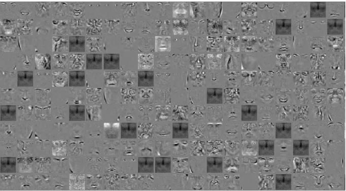
DAE was trained on TFD. Experiments show that higher corruption level of the inputs (ex: p=0.4) leads to better filters and classification results than smaller values. DAE was trained using cross-entropy error function and mean square error. Practically, it seems that cross entropy with sigmoid activation function on the hidden units gives better results than using mean square error. It is important to mention that cross-entropy is the logical error function to be used on binary dataset but TFD data is not binary, so using cross-entropy on TFD is a hack, although it is practically helpful. Figure 9 shows part of the learned filters. Unfortunately, there are many noisy filters which seem to learn nothing. The classification accuracy obtained with a linear SVM trained on the hidden representation was 76.1% (by comparison, when trained on raw image pixels they yield 71.5%). The incoming weights for each neuron were initialized as in [38] i.e. drawn from distribution:

(43)

√

Where is the number of units in the ( ) layer and is the number of units in

the layer( ).

Figure 9: Some filters learned by a DAE on TFD

Since some weights have larger magnitude than others, the convergence to good filters can be faster for some while slower for others. To minimize the impact of this phenomenon, starting with small weights was investigated (i.e. the norm of the weight vector for each unit is less than n, where n is a hyper-parameter) such that update rule will prevent fast change (assuming small learning rate). Figure 10 shows the effect on the resulting learned filters with

(44)

= 0.5. Some filters appear sharper than before (mouth and eye edges). The classification performance was a little bit lower than with regular DAE (75.39%).

Figure 10: DAE filters with small weights initialization

5.2 Dropout with maximum weight

Experiments were performed to study the effect of the maximum weight hyper-parameter (n) on learned filters and on classification results with dropout. The experiments were done by choosing some fixed values for all hyper-parameters except n, and then changing the value of n only.

(45)

(a)

(46)

Figure 11: Effect of maximum weight on TFD using dropout. (a) small weight magnitude (b) bigger weigh magnitude

(a)

(47)

Figure 12: The effect of maximum weight with Dropout on MNIST. (a) small weight magnitude (b) bigger weigh magnitude

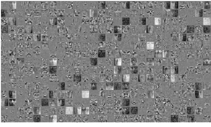
Figure 11 and Figure 12 show the effect of applying maximum weight with dropout and visualize the good effect of having small maximum weight constraint. It seems that the learning procedure forces each neuron to choose a few big weight values and keep them small for the other weights yielding more localized filters, such as the crisp edges which are pretty obvious in Figure 12 (a). The classification accuracy ,with the error in brackets for MNIST, was:

small maximum weight (0.1)

big maximum weight (1.00)

With hyper-parameter search

MNIST 98.4% (1.6) 98.32 % (1.68) 98.59 % (1.41)

TFD 71.21 % 71.92 % 73.35 %

Table 2: The effect of applying maximum weight on classification for both TFD and MNIST using dropout

It seems that having small maximum weight was helpful on MNITS but not on TFD. In addition, dropping hidden units made classification result worse on TFD (73.35% in Table 2 compared to 76.1%).

5.3 Using the same dropout mask on the batch

The stochastic process used by dropout is very useful but we believe it should be used differently. Using a dropout mask for each sample (even when we use batch learning) is not the good thing to do because each example tells the neuron to learn something very different which we guess is the main reason for some neuron to learn nothing. The alternative way is to use the same dropout mask for each mini-batch. This will help each neuron to learn on a

(48)

specific pattern on many examples (instead of one example). Using the same dropout mask for a sample batch can be though as training an ensemble of models using bagging such that each model is trained on different samples (instead of one when the batch size is one).

The idea was tested on TFD by varying the batch size (see Figure 13).

(49)

(b)

Figure 13: Filters on TFD when the same dropout mask is used for the whole batch. (a): Batch size equal 20

(b): Batch size equal 10

The good news is that using this technique gives better classification results than any technique described before. The table below shows the effect of varying the batch size.

Batch Size Classification Accuracy

10 77.42 %

20 76.34 %

40 75.5 %

60 75.0 %

100 74.67 %

(50)

According to the conducted experiments, the best classification result was 77.42 % with batch size 10. For the sake of comparison, when the different dropout masks were used with batch size 20 the classification result was (73.34%), so 3% gain was achieved when the same mask was used for batch size 20 for this specific dataset.

5.4 Manifold Autoencoder

A lot of time was spent on this part of the experiments. The manifold autoencoder (described in section 4.1) was tested on the MNIST dataset using different configurations. In practice, using sigmoid activation function in the hidden proved to be a very bad choice, the obtained filters were very noisy and the learning was too slow. For this reason, rectifiers with mean square error were tried instead of sigmoid. In this way, we were able to minimize the three terms in the cost function after training on a very small number of examples (e.g. 1000). In order to analyse the dynamics of training in this model, a simple tool was created to monitor the square of the reconstruction error, the trace of the Jacobian, the intrinsic dimension error (which can be calculated from the trace of the Jacobian), the cost of how sharp the spectral curve is and the max, mean of the weight matrix and the mean of the gradients with respect to the weights. Figure below shows the plot of the four values values. While the x-axis corresponds to the number of seen examples (the progress of training), the y-axis shows the value of the measured criteria.

(51)

(52)

The reconstruction error seems to be around seven after being trained on 15800 samples. The intrinsic dimension value (the trace of the Jacobian) is very close to the pre-defined hyper-parameter chosen value (c = 50) which makes the intrinsic dimension error (how far it is from c for every sample) small. On the other hand, the sharpness error which makes the spectral curve decrease immediately is close to one (check Figure 17).

After training the AE, the mean and the standard deviation of the activation of the hidden units (Figure 15 red and blue curves respectively) were evaluated on random samples in order to be sure that the units are not dead (doing something meaningful). The mean of activation was plotted after sorting the mean activation of the units in ascending order.

Figure 15: The mean and standard deviation of the hidden units activation.

The figure below shows the qualitative reconstruction of images on which the model was not trained together on with some of the learned filters.

(53)

Figure 16: The reconstruction of some MNIST digits and some of the learned filters

Finally the spectral curve was evaluated. Note that we used c = 50 as the hyper-parameter giving the target intrinsic dimension. The figure below shows how the sharpness constrained is satisfied. The criterion optimized (section 4.1 equation 1) indeed yields a spectrum of the desired shape.

(54)

Figure 17: The spectral curve of the Jacobian on MNIST.

Unfortunately, the classification result on the hidden representation using SVM is (98.11) which is worse than the result of kernel SVM on raw pixels (98.6). This means that the non-linear transformation achieved by the novel auto-encoder was not useful enough. Theoretically the model should work fine but it seems that there are some details, e.g. hyper-parameters, which should be studied more carefully in the future.

(55)

5.5 Semi Supervised Denoising Autoencoder (SSDAE)

SSDAE was tested on several datasets: TFD (all folds), MNIST and CIFAR100 which is a 32x32 colour images dataset that has 100 classes containing 600 images each for natural images (e.g fish, flowers, trees, …etc.). There are 500 training images and 100 testing images per class [39].

Both DAE and SSDAE with one hidden layer, rectifier activation function, and tied weights were launched and the learned hidden representation was finally fed to a linear SVM. For simplicity, all experiments used a diagonal matrix A (although a more general matrix form could conceivably be used). Two different heuristics were used to build it:

 Hand-crafted A using a naïve heuristic based on prior knowledge of the task:

─ For MNIST we assigned each pixel a weight proportional to its probability of being active as measured on average in the training set. This means that background pixels which are always zeros on all digits will have no effect on the cost function.

─ For TFD, whose examples are frontal aligned faces, we reasoned that mouth and eyebrow regions were more important than others (like cheeks) for figuring out the emotion. So we attributed pixels in these regions a weight of 1, while all others were given a weight of 0.5.

 A is chosen based on the importance given to each input feature in the solution learned by a random forest classifier [40] .In random forests, each tree in the ensemble is built from a sample drawn with replacement (i.e., a bootstrap sample) from the training set. In addition, when splitting a node during the construction of the tree, the split that is chosen is no longer the best split among all features. Instead, the split that is picked is the best split among a random subset of the features. As a result of this randomness, the bias of the forest usually slightly increases (with respect to the bias of a single non-random tree) but, due to averaging, its variance also decreases, usually more than compensating for the increase in bias, hence yielding an overall better model..

(56)

Figure 18: Pixels Importance for TFD and MNIST using Random Forests

Table 4 shows how SSDAE with random forest gives the best classification result on the tested datasets. Note that using SSDAE on both TFD and MNIST gave better classification results than DAE. On the other hand, no tangible benefit was achieved on CIFAR 100. This result is not surprising since TFD and MNIST information are concentrated on some pixels more than others (since TFD and MNIST are relatively aligned) while it is not as clearly the case in CIFAR 100.

TFD (accuracy %)

Fold 0 Fold 1 Fold 2 Fold 3 Fold 4 Final SSDAE (naïve) 77.3 75.97 75.81 76.89 73.11 75.82 % ( ) SSDAE (random forest) 79.57 78.8 76.89 78.08 73.11 77.29 % ( ) DAE 77.3 76.56 75.93 76.17 72.38 75.67 % ( )

(57)

MNIST (error rate %) SSDAE (random forest) 1.17 %

SSDAE (naïve) 1.24 %

DAE 1.28 %

CIFAR 100 (accuracy %) SSDAE (random forest) 29.98 %

DAE 29.52 %

Table 4: Comparision between DAE and SSDAE classification on TFD, MNIST and CIFAR100. Numbers in paranthesis are standard deviation of accuracy on the TFD splits.

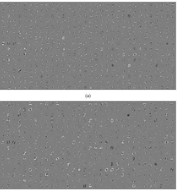
The figure below shows some of the learnt filters for MNIST and the reconstruction for some images that has never been seen during training. Note how the reconstruction is noisy for background pixels that have zero importance (Figure 18).

(58)

Figure 19: Some MNIST filters trained using SSDAE and the reconstruction of some images.

Finally, a simple experiment was done to check if assigning SSDAE parameters to a neural network and fine-tune it helps improving the learning process. To check this hypothesis, we trained an SSDAE on 9*9 TFD patches, gave the best results on similar problems when we trained on TFD, that are sampled from the pixels importance distribution. Generally, training on image patches is done by sampling random patches from the whole image (e.g. training in a convolutional manner). Here, a different approach was used. Since each pixel has its own importance, this importance defines a probability distribution over pixels by dividing each pixel importance on the summation of all pixels importance. This means that our pre-training phase will be trained on specific regions (patches) of the images more than others. Figure 20 shows an 8*7 image with the importance of each pixel (the sum adds to one). If we want to choose a pixel using the pixels importance distribution we will sample the pixel that has 0.1 importance value (red) more than the pixel having 0.025 importance (green). Now if we have 3*3 patches to pre-train on, the patch defined by the bold border will be seen by the classifier more than the patch defined by the dotted border.

Figure 20: An image with pixels importances showing how dark border patch is sampled more than the dotted border patch due to higher center value.

Then we used these parameters to initialize one hidden layer convolutional net. The reason behind this experiment is to compare with [41] where a slightly different CAE variation

(59)

that disentangles the factors of the hidden units was trained on TFD random patches. The CAE variation parameters were used as initialization for a convolutional net. The CAE variation yielded around 1% accuracy boost on the classification compared to CAE only. In our experiment, we did not use anything to disentangle the factors of variation. All we did was using the proposed SSDAE for pre-training. The results are shown in the table below:

TFD

Fold 0 Fold 1 Fold 2 Fold 3 Fold 4 Final SSDAE 85.42 84.33 85.03 85.03 82.48 84.48 %

( )

(Rifai et al,2012) - - - 85.00 %

Table 5: Conv net pre-trained using SSDAE on TFD folds.

Although SSDAE pre-training did not reach the 85%, the performance boost obtained with the much simpler principle underlying the modification we propose in the SSDAE is nevertheless remarkable. Note also that feeding the hidden representation of SSDAE directly to linear SVM shows that SSDAE is able to extract better features than the DAE, yielding higher classification accuracy. As we mentioned earlier, the new criterion can be tested with any auto-encoder type, as it affects only the reconstruction error term.

(60)

Chapter 6: Convolutional Net Experiments

This section will be devoted to experiments mainly conducted on TFD in order to build a robust model that can be used in the live demo.

Different convolutional nets with different hyper-parameters were tested. The best way to present these experiments is using chronological order which reflects how the model was improved and how ideas were built. Models are going to be numbered in order to refer to them later. Note that all models are trained using early stopping and adaptive learning rate unless stated otherwise. The model was also trained on distorted and mirrored images in order to increase the number of training examples. First of all, a convolutional net with 15 feature maps, one sigmoid hidden layer followed by a softmax layer was trained on TFD. The average error on five folds with the standard deviation was:

Model 1

Fold 0 Fold 1 Fold 2 Fold 3 Fold 4 Average Error Overall accuracy 16.25% 21.55 % 20 % 18.92 % 24.82 % 20.30% ( ) 79.69%

Table 6: ConvNet classification result on TFD

With the same architecture, the network was retrained by adding an L2 weight decay regularization, which enhanced the performance: