Detailed 2D numerical modeling for flood extension forecasting

Detailed 2D numerical modeling for flood extension forecasting

S. Erpicum, B.J. Dewals

, P. Archambeau, S. Detrembleur & M. Pirotton

Applied Hydrodynamics and Hydraulic Constructions Research Unit HACH, MS²F, ArGEnCo Department, University of Liege, Liege, Belgium

*

Belgium National Fund for Scientific Research (F.R.S. – FNRS)

ABSTRACT

In the global framework of recurrent large flood events all over the world and in Europe in particular, relevant and detailed inundation maps represent a tool of prime interest for decision makers, emergency services or insurance companies. In 2003 in Belgium, following a Regional Government decision, hydraulic 2D numerical modelling has been chosen to compute inundation maps on 800 km of the main rivers of the Walloon Region, using high resolution Digital Elevation Models. The present paper covers a detailed description of the state-of-the-art 2D finite volume model used to fulfil this task. As a part of this project, the model has been extensively validated by comparisons with observations during recent real flood events. It shows a very good agreement with observations, in particular regarding free surface elevations.

Following this first step toward flood management, the Belgian National project “ADAPT” is presented. It aims to develop an efficient decision support tool for the integrated assessment of adaptation measures against climate change induced flooding. In this scope, the model has been applied to predict inundations induced by floods, taking into account different climate change scenarios. The results of these simulations serve as input for a subsequent economic, social and ecological analysis by other scientific research teams.

Keywords: SWE, finite volume, DEM, inundation mapping, climate change

1 INTRODUCTION

In the global framework of recurrent large flood events all over the world and in Europe in particular, relevant and detailed inundation maps represent a tool of prime interest to help decision makers in defining land use and housing policies, to inform people living in flood risk zones, to improve emergency planning and to help insurance companies to assess the risks associated with flooding. To be usable in practise, such maps should however be drawn in a scientific and objective manner. They should also cover a large range of probabilistic flood events, taking into account possible climate evolution, and not only

represent well documented extreme events from the past. Finally, they have to be easy to update regarding significant changes in the river topography or floodplain characteristics.

In this scope, hydraulic numerical modelling can provide relevant and reliable results, especially when the solvers are able to use the accurate and very dense topographic information provided today by high resolution Digital Elevation Models (DEMs) derived form airborne lidar or on boat sonar (McMillan and Brasington (2007)). A significant evolution of the flood inundation numerical models using such DEMs has been observed over the last decades. Bates and De Roo (2000) clearly summarized this evolution, starting with planar water surface model without channel or

floodplain routing (Priestnall et al. (2000)) up to 2D models providing a full solution of the Saint-Venant equations on the whole inundated area (Archambeau et al. (2004), Erpicum et al. (2007) or Mignot et al. (2006) for example), passing by coupled approaches applying different more or less sophisticated models in the channel and the floodplain (for example Bates and De Roo (2000), McMillan and Brasington (2007)).

The application of full 2D models on the whole inundated area provides reliable distributed results, such as water heights and velocity fields, even in dense urban areas (Mignot et al. (2006)). These results are of prime interest to estimate the damage caused by the floods (Dutta et al. (2003)), and thus the risk associated to flooding.

Once the parameters of the model have been calibrated, and especially roughness coefficient, inundations modelling can be carried out for a set of pertinent probabilistic extreme events in order to fully characterise the so-called “inundation hazard” along a river (HACH (2006)).

McMillan and Brasington (2007) point out that the main drawback of actual flow solvers lies in their inability to make optimal use of the very dense topography information provided today by airborne lidar for example. In this paper, a full 2D hydraulic numerical model is presented, which has been used to compute flood inundation maps on 800 km of main rivers in the Walloon Region in Belgium with a spatial resolution as fine as 2 to 2 meters. Coupled with high resolution DEMs, the solver allows computing inundation maps at the scale of the streets and buildings in urban area for example. The simplicity and the efficiency of the finite volume numerical scheme make indeed the model able to solve the classical shallow water equations (SWE) on computation grids counting for as much as one million meshes (3 millions unknowns) using standard computers (3.4 Ghz - 4Gb RAM).

Following the description of the solver, some validation examples and applications for flood inundation mapping are presented.

In a second time, the Belgian National project “ADAPT” is presented. This project aims to develop an efficient decision support tool for the integrated assessment of adaptation

measures against flooding induced by climate change. In this framework, for selected case studies, the above described 2D model has been used to predict inundations induced by floods of two different return periods (25 years and 100 years) and for four different climate change scenarios (ranging between a 5% and a 30% increase in the peak discharge corresponding to the present base scenario). The results of these simulations serve as input for a subsequent economic, as well as social and ecological, analysis carried out by other scientific research teams.

2 HYDRAULIC MODEL DESCRIPTION

2.1 Mathematical model

The 2D hydraulic model is based on the two-dimensional depth-averaged equations of volume and momentum conservation (SWE). In the “shallow-water” approach, the only assumption states that velocities normal to a main flow direction are smaller than those in this main flow direction. As a consequence, the pressure field is found to be almost hydrostatic everywhere.

The large majority of flows occurring in rivers, even highly transient, can be reasonably seen as shallow, except in the vicinity of some singularities (e.g. weirs). Indeed, vertical velocity components remain generally low compared to velocity components in the horizontal plane and, consequently, flows may be considered as mainly two-dimensional. Thus, the approach presented in this paper is suitable for many of the problems encountered in river management, and especially inundation mapping.

The conservative form of the depth-averaged equations of volume and momentum conservation can be written as follows, using vector notations: 0 f d d t x y x y ∂ ∂ ∂ ∂ ∂ + + + + = − ∂ ∂ ∂ ∂ ∂ f g s f g S S

[

]

where is the vector of the

conservative unknowns. f and g represent the advective and pressure fluxes in directions x and y, while fd and gd are the diffusive fluxes:

2 1 2 2 hu hu gh huv ⎛ ⎞ ⎜ ⎟ =_⎜ + _⎟ ⎜ ⎟ ⎝ ⎠ f , 2 1 2 2 hv huv hv gh ⎛ ⎞ ⎜ ⎟ = ⎜ ⎟ ⎜ ₊ ⎟ ⎝ ⎠ g (2) d 0 x xy h σ ρ _τ ⎛ ⎞ ⎜ ⎟ = − ⎜ ⎟ ⎜ ⎟ ⎝ ⎠ f , d 0 xy y h τ ρ _σ ⎛ ⎞ ⎜ ⎟ = − ⎜ ⎟ ⎜ ⎟ ⎝ ⎠ g (3)

S0 and Sf designates respectively the

bottom slope and the friction terms:

[

]

t represents the time, x and y the space

coordinates, h the water depth, u and v the depth-averaged velocity components, zb the

bottom elevation, g the gravity acceleration, ρ the density of water, τbx and τby the bottom

shear stresses, σx and σy the turbulent normal

stresses, and τxy the turbulent shear stress.

Consistently with Hervouet (2003),

( ) (2 )2

b b

1 z x z y

ΔΣ = + ∂ ∂ + ∂ ∂ (6)

reproduces the increased friction area on an irregular (natural) topography (Dewals (2006)).

2.2 Friction modelling

The bottom friction is conventionally modelled thanks to an empirical law, such as the Manning formula. The model enables the definition of a spatially distributed roughness coefficient to represent different land-uses, floodplain vegetations or sub-grid bed forms… Besides, the friction along side walls is reproduced through a process-oriented formulation developed by the authors (Dewals (2006)): 2 2 2 2 b b 4 / 3 1/ 3 1 4 3 x x N x k n n gh u u v u h h τ ρ = ⎡ = ⎢ + + _Δ ⎣

∑

∑

where the Manning coefficient nb and nw

characterize respectively the bottom and the side-walls roughness. Those relations are particularized for Cartesian grids exploited in the present study.

The internal friction should be reproduced by applying a proper turbulence model. Several ones have been implemented and tested in the solver, starting from rather simple algebraic expressions of turbulent viscosity to a depth-integrated k-ε type model involving additional partial differential equations (Erpicum (2006)). Nevertheless, for the computations presented in this paper, no turbulence model has been used. All friction effects are thus globalized in the bottom and wall friction term in a fitted value of the roughness coefficient.

2.3 Grid and numerical scheme

The solver includes a mesh generator and deals with multiblock grids. Within each block, the grid is Cartesian to take advantage of the lower computation time and the gain in accuracy provided by this type of structured grids compared to unstructured ones.

The multiblock feature increases the surface of domains discretizable with a constant cells number while enabling local mesh refinements close to interesting areas. It is thus a solution to solve the main drawback of Cartesian grid, i.e. the high number of cells they need to reach a fine enough discretization.

In addition, an automatic grid adaptation technique restricts the simulation domain to the wet cells to decrease the number of computation elements. Besides, wetting and drying of cells is handled free of volume and momentum conservation errors by the way of an iterative resolution of the continuity equation prior to any evaluation of the momentum equations (Erpicum et al. (2004)).

The space discretization of Eq. (1) is performed by means of a finite volume scheme. This ensures a proper mass and momentum conservation, which is a prerequisite for handling reliably discontinuous solutions such as moving hydraulic jumps.

As a consequence, no assumption is required as regards to the smoothness of the solution. Reconstruction at cells interfaces can be performed constantly or linearly, in conjunction with slope limiting, leading in the second case to a second-order spatial accuracy.

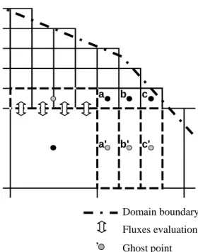
In a similar way, variables at the border between adjacent blocks are reconstructed linearly, using in addition ghost points as

Figure 1: Border between two adjacent blocks on a Cartesian multiblock grid

depicted in figure 1. The value of the variables at the ghost points is evaluated from the value of the subjacent cells. Moreover, to ensure conservation properties at the border between adjacent blocks and thus to compute accurate volume and momentum balances, fluxes related to the larger cells are computed at the level of the finer ones.

Appropriate flux computation has always been a challenging issue in computational fluid dynamics. The fluxes f and g are computed by a Flux Vector Splitting (FVS) method developed by the authors. Following this FVS, the upwinding direction of each term of the fluxes is simply dictated by the sign of the flow velocity reconstructed at the cells interfaces. It can be formally expressed as follows:

2 2 0 ; 2 0 hu hu gh huv + − ⎛ ⎞ ⎛ ⎜ ⎟ ⎜ =_{⎜ ⎟} =_⎜ ⎜ ⎟ ⎜ ⎝ ⎠ ⎝ f f ⎞ ⎟ ⎟ ⎟ ⎠ (9) 2 2 0 ; 0 2 hv huv hv gh + − ⎛ ⎞ ⎛ ⎜ ⎟ ⎜ =_{⎜ ⎟} =_⎜ ⎜ ⎟ ⎜ ⎝ ⎠ ⎝ g g ⎞ ⎟ ⎟ ⎟ ⎠ (10)

where the exponents + and - refer to, respectively, an upstream and a downstream evaluation of the corresponding terms. A Von Neumann stability analysis has demonstrated that this FVS leads to a stable spatial discretization of the terms ∂ ∂f x and ∂ ∂g y in

Eq. 1 (Dewals (2006)). Due to their diffusive nature, the fluxes fd and gd are legitimately

evaluated by means of a centred scheme.

Besides requiring a low computation cost, this FVS offers the advantages of being completely Froude independent and of facilitating a satisfactory adequacy with the discretization of the bottom slope term. This FVS has already proved its validity and efficiency for numerous applications (Archambeau et al. (2004), Dewals (2006), Dewals et al. (2006), Erpicum et al. (2004), Erpicum (2006), Erpicum et al. (2006), Erpicum et al. (2007), HACH (2006)).

a b c a' b' c' Domain boundary Fluxes evaluation 2.4 Topography gradients ’ _{Ghost point}

The discretization of the topography gradients is always a challenging task when setting up a numerical flow solver based on the SWE. The bed slope appears as a source term in the momentum equations. As a driving force of the flow, it has however to be discretized carefully, in particular regarding the treatment of the advective terms leading to the water movement, such as pressure and momentum.

In the model presented in this paper, according to the FVS characteristics, a suitable treatment of the topography gradient source term of Eq. 4 is a downstream discretization of the bottom slope and a mean evaluation of the corresponding water heights (Erpicum (2006)). For a mesh i and considering a constant reconstruction of the variables, the bottom slope discretization writes:

(

)

(

)

where subscript i+1 refers to the downstream mesh along x- or y- axis.

This approach fulfils the numerical compatibility conditions defined by Nujic (1995) regarding the stability of water at rest. The final formulation is the same as the one proposed by Soares Frazão (2000) or Audusse (2004).

The formulation is suited to be used in both 1- and 2D models, along x- and y- axis. Its very light expression benefits directly from the simplicity of the original spatial discretization scheme.

Nevertheless, the formulation of Eq. 11 constitutes only a first step toward an adequate form of the topography gradient as it is not entirely suited regarding water in movement over an irregular bed. The effect of kinetic terms is not taken into account and, as a consequence, bad evaluation of the flow energy evolution can occur when modelling flow over a variable topography (Erpicum, (2006)).

2.5 Time discretization

Since the model is applied to compute steady-state solutions, the time integration is performed by means of a 3-step first order accurate Runge-Kutta algorithm, providing adequate dissipation in time. For stability reasons, the time step is constrained by the Courant-Friedrichs-Levy condition based on gravity waves. A semi-implicit treatment of the bottom friction term is used, without requiring additional computational costs.

Slight changes in the Runge-Kutta algorithm coefficients allow modifying its dissipation properties and make it suitable for accurate transient computations.

2.6 Boundary conditions

For each application, the value of the specific discharge can be prescribed as an inflow boundary condition. Besides, the transverse specific discharge is usually set to zero at the inflow even if its value can also be prescribed to a different value if necessary. In case of supercritical flow, a water elevation can be provided as additional inflow boundary condition.

The outflow boundary condition may be a water surface elevation, a Froude number or no specific condition if the outflow is supercritical. At solid walls, the component of the specific discharge normal to the wall is set to zero.

2.6 Other features

The herein described model constitutes a part of the modelling system “WOLF”, developed at the University of Liege. WOLF includes a set of complementary and interconnected

modules for simulating free surface flows: process-oriented hydrology, 1D & 2D hydrodynamic, sediment (Dewals (2006)) or pollutant transport, air entrainment, as well as an optimisation tool based on Genetic Algorithms (Erpicum, (2006)).

Other functionalities of WOLF 2D include the use of moment of momentum equations (Dewals (2006)), the application of the cut-cell method (Erpicum et al. (2006)), as well as computations considering vertical curvature effects by means of curvilinear coordinates in the vertical plane (Dewals et al. (2006)).

A user-friendly GIS interface, entirely designed and implemented by the authors (Archambeau (2006)), makes the pre- and post-processing operations very convenient. Import and export operations are easily feasible from and to various classical GIS tools. Different layers of maps can be handled to analyse information related to the topography, the ground characteristics, the vegetation density and the hydrodynamic fields.

3 FLOOD INUNDATION MAPPING

3.1 Topography data

In Belgium, a few years ago, the Walloon Ministry of Facilities and Transport (MET), and in particular the Service of Hydrological Studies (SETHY), acquired an accurate DEM on the floodplains in the whole South part of the country. An airborne laser has been used to measure the topography of the floodplain of the main rivers network and an echo-sonar technique has been applied to characterise the bathymetry of the main channel on navigable rivers.

Consequently, the poor and inaccurate topography information available for many years, i.e. 30 m of plan resolution with a precision of several meters in altitude, has been replaced by an exceptional data set since the laser and sonar precision in altitude is 15 cm and the information density is one point per square meter.

This huge improvement in the quality of the main data set enables to focus on proper physical values of the roughness coefficient

rather than using it to assess the effect of blockage by buildings or of large irregularities of the topography. It allows also refining the flood extension forecasting at the scale of houses and streets.

Regarding smaller non navigable rivers, cross sections information can be efficiently interpolated to generate the main bed bathymetry and to complete the laser data.

However, in this case, a special care has to be paid to possible singularities in the river bed and the DEM resulting from the interpolation procedure has often to be completed to represent the whole of the river bed details. This last procedure can be even more important and time consuming when the cross sections information dates from tens of years, as it is generally the case in several European countries.

This last point underlines the importance of the accuracy and especially of the update of the data to provide reliable numerical results. It makes also very useful the storage of all the data sets to be able to quickly pick them up to update the maps to take into account modifications in the DEM.

3.2 Validation and application on 800 km of rivers in Belgium

Following a Regional Government decision in 2003, the solver WOLF2D, presented in this paper, has been chosen to be used to compute the official inundation maps on 800 km of the main rivers of the Walloon Region in Belgium. For each river, the following procedure has been followed:

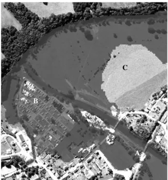
Figure 2: Real event on the river Lesse – January 28th, 1995 – Q = 180 m³/s

• Complete DEM building on a 1 to 1 m grid (channel and floodplain) from lidar data and echo sonar or cross section ones,

• In situ validation of the topography singularities geometry and characteristics, • Modelling of the best documented

historical flood event for calibration and validation on 2 to 2 or 5 to 5 m grid depending on the river width,

• Computation of the inundation maps for constant statistical flood discharge values with a 25-, 50- and 100-year return period on the same grid.

Figures 2 and 3 illustrate the results of the validation stage at Wanlin, on the river Lesse, during the flood of January 28th 1995 (Q = 180 m³/s – Return period is +/- 15 years). The numerical results (Fig. 3) represent the flood extension, which is in very good agreement with the picture of the real event (Fig. 2). The caravans in the campsite have been removed from the DEM as the water can flow under them (Point B – Fig. 2 and 3).

Figure 3: Computation results in the river Lesse for the flood of January 28th, 1995 – Q = 180 m³/s

C

B

A

B _C

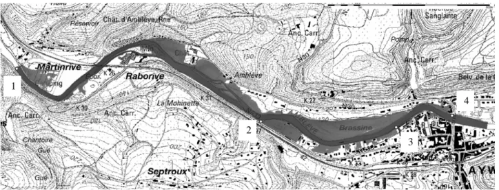
A _{In the same scope, Table 1 and Fig. 4 show}

the comparison between water elevation surveys realized during the flood of December 1993 on the river Amblève and the numerical computation of the same event.

Figure 4: Numerical results of the December 21th, 1993 flood extension computation on a 3 km long reach of the river Amblève – Q = 298 m³/s – Location of the 4 points for water surface elevation comparison

1

2

3

4

Table 1: Comparison between water elevations survey and numerical results on the river Amblève – Event of Decembre 21th, 1993 – Q = 298 m³/s

Real event Numerical results Location (m) (m) 1 Martinrive bridge (boundary condition) 112.77 112.77 2 Downstream of the football field 118.38 118.4 3 Aywaille boarding school 119.81 119.85 4 Bridge of Aywaille 120.81 120.85

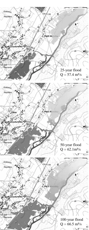
Regarding flood mapping, Figure 5 illustrate the results of the computation on the river Dendre near Papignies with the extension maps for events with a 25-, 50- and 100-year return period (discharge of respectively 57.4, 62.1 and 66.5 m³/s). These final results in terms of water heights, together with the distributed mean velocity fields, fully characterise the inundation hazard.

4. FURTHER USE: ADAPT PROJECT

4.1 Context

In the framework of the Belgian national research project “ADAPT - Towards an integrated decision tool for adaptation measures”, the hydrodynamic model WOLF 2D also serves as a core component of a decision-support system dedicated to the

integrated evaluation of flood protection measures in the context of increased flooding hazard as a result of climate change (De Groof et al (2006)). This tool is based on a combination of cost-benefit analysis (CBA) and multi-criteria analysis (MCA), taking into consideration hydraulic, economic, social and ecological indicators.

The following paragraphs describe how the hydrodynamic model WOLF 2D is implemented within the system, with a focus on the selection of modelling scenarios and on the simulation results.

4.2 Preliminary steps

In order to demonstrate the efficiency of the decision-support system and to facilitate its refinement, the methodology has first been tested on case study areas, which include two distinct reaches of the river Ourthe in the Meuse basin (Belgium).

Besides, prior to evaluating the benefits of different adaptation measures, a preliminary step consisted in determining how inundation hazard is likely to be modified by climate change. More precisely, for different return periods of floods and for several climate change scenarios, hydrodynamic simulations have been run with WOLF 2D in order to identify which modifications climate change will cause to inundation extents as well as to water depths and flow velocities in the floodplains.

Figure 5: Flood extension maps on the river Dendre near Papignies for three statistical extreme floods

4.3 Main modelling assumptions

Results of Global Circulation Models (GCM) and Regional Climate Models (RCM) provide estimates of the potential increase in precipitation (winter and summer) and potential changes in evapotranspiration as a result of

climate change. Those predicted changes are affected by a significant level of uncertainty due to the climate models themselves and, to an even greater extent, to the discrepancies in the scenarios used for running those climate models (IPCC (2007)).

Moreover, translating those changes in precipitation and evapotranspiration into changes in river discharges is also a challenging task, since the catchment response depends on many factors such as the land roughness and permeability, the rainfall duration, … Therefore, at the first stage of the ADAPT project, simple assumptions have been considered regarding the expected changes in the peak discharges of the river Ourthe as a result of climate change. Indeed, according to a comprehensive literature review (De Groof et al (2006), Dewals et al (2007)), an increase by 10% of flood discharge may be regarded as reasonable. Moreover, in order to evaluate the sensitivity of the results with respect to this perturbation factor on the discharge, increases by 5% and by 15% have also been considered. Besides, a more extreme case has been simulated as well (+30%). All those assumptions will eventually be confirmed and refined by comparison with the output of a hydrological model (De Groof et al (2006)).

25-year flood Q = 57.4 m³/s

50-year flood Q = 62.1m³/s

4.4 Hydrodynamic simulations and results

By means of hydrodynamic simulations with WOLF 2D, the assumed modifications in the expected discharges have been translated into updated evaluations of flooding extent and characteristics for the two considered reaches of River Ourthe. The study has been performed for two different return periods, namely 25 and 100 years, for which the best adaptation strategies will most likely be completely different, due to the differences in inundated areas and in probability of occurrence.

100-year flood Q = 66.5 m³/s

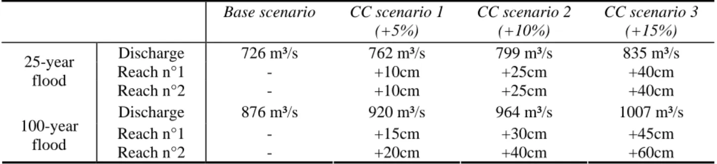
Table 2 summarizes the different hydraulic simulations performed for the two considered reaches. It also provides averaged values of the change in water depths; while detailed results are available in the form of updated inundation maps (e.g. increase in water depth compared to the base scenario). As mentioned above, in addition, a more extreme simulation scenario (+30%) has also been considered.

It is found that the results can be very sensitive to the perturbation factor affecting the discharge, due for instance to the reduced efficiency of flood protection structures (e.g. dikes) above a threshold value of discharge (design discharge). Moreover, the complexity of the flow fields represented on the inundation maps recalls the relevance of exploiting a fully two-dimensional flow model.

Results have also been provided in the form of updated inundation maps, indicating, for each return period and each climate change scenario, the 2D distribution of water depth in the floodplains, flow velocity and increase in water depth compared to the base scenario. This set of results served as an input for the subsequent economic, as well as social (Coninx and Bachus (2007)) and ecological, analysis conducted by means of the corresponding modules of the decision-support system.

5. CONCLUSIONS

Following a rigorous systematic methodology, the application of a conscientiously developed 2D finite volume free surface flow solver using high resolution DEMs allows obtaining reliable and finely distributed flood extension maps on 800 km of the main rivers of the South part of Belgium. The results of the computations fully characterise the inundation hazard, which is a prerequisite to further flood risk assessment.

Beyond these useful results for risk analysis and land use policies, the fine grid of the simulation associated with the considerable elevation precision allow very precise impact and remediation studies, and such a distributed approach plays thus the role of a genuine tool to help decision makers.

One of the perspectives of improvements in the near future is to link these flow simulations with hydrological computations of the whole river watershed to predict the flood extension from real time rain data.

Table 2: Mean change in water depth induced by Climate Change (CC) for two different return periods.

Base scenario CC scenario 1

(+5%) CC scenario 2 (+10%) CC scenario 3 (+15%) Discharge 726 m³/s 762 m³/s 799 m³/s 835 m³/s Reach n°1 - +10cm +25cm +40cm 25-year flood Reach n°2 - +10cm +25cm +40cm Discharge 876 m³/s 920 m³/s 964 m³/s 1007 m³/s Reach n°1 - +15cm +30cm +45cm 100-year flood _{Reach n°2 - +20cm +40cm +60cm} ACKNOWLEDGEMENT

The authors gratefully acknowledge the Walloon Ministry of Facilities and Transport (MET) who provided the DEMs information.

Part of this research was carried out on behalf of the Belgian Science Policy (BELSPO), in the framework of the program “Science for a Sustainable Development”.

NOTATIONS

f = x-component of advective terms vector fd = x-component of diffusive terms vector g = gravity acceleration

g = y-component of advective terms vector gd = y-component of diffusive terms vector h = water height

i = reference cell index

i+1 = cell downstream of i cell index

nb = Manning coefficient of the river bottom

nw = Manning coefficient of the side walls

Q = Discharge s = unknowns vector

S0 = bottom slope terms vector

Sf = friction terms vector t = time

u = average fluid velocity along x-direction v = average fluid velocity along y-direction x = x Cartesian coordinate

Z = free surface elevation

zb = bottom elevation

ΔΣ = factor of increased friction area

ρ = water density

σx = turbulent normal stresses in x-direction σy = turbulent normal stresses in y-direction τbx = bottom shear stress along x-direction τby = bottom shear stress along y-direction τxy = turbulent shear stress

REFERENCES

Archambeau P., Dewals B.J., Detrembleur S., Erpicum S., and Pirotton M. 2004. A set of efficient numerical tools for floodplain modeling. Shallow Flows, G.H. Jirka and W.S.J. Uijttewaal (eds), Balkema: Leiden, 549-557.

Archambeau P., Dewals B.J., Erpicum S., Detrembleur S., and Pirotton M. 2004. New trends in flood risk analysis: working with 2D flow models, laser DEM and a GIS environment. Proc. Of 2nd Int. Conf. on Fluvial Hydraulics: Riverflow 2004, M. Greco, A. Carravetta and R. Della Morte (eds), Vol. 2. Balkema: Leiden, 1395-1401.

Archambeau P. 2006. Contribution à la modélisation de

la genèse et de la propagation des crues et inondations. Unité d’Hydrodynamique Appliquée et

des Constructions Hydrauliques, Thèse de doctorat, Université de Liège, Liège. 423 p.

Audusse E. 2004. Modélisation hyperbolique et analyse

numérique pour les écoulements en eaux peu profondes. Laboratoire Jacques-Louis Lions, Thèse

de doctorat, Université Paris VI – Pierre et Marie Curie, Paris. 193 p.

Bates P.D., and De Roo A.P.J. 2000. A simple raster-based model for flood inundation simulation. Journal

of Hydrology, Vol. 236, 54-77.

Coninx I. and Bachus K. 2007. Integrating social vulnerability to floods in a climate change context.

Proc. Of Int. Conf. on adaptive and integrated water management, coping with complexity and uncertainty. Basel, Switzerland.

De Groof A., Hecq W., Coninx I., Bachus K., Dewals B., Pirotton M., El Kahloun M., Meire P., De Smet L., and De Sutter R. 2006. General study and evaluation

of potential impacts of climate change in Belgium. ADAPT - Towards an integrated decision tool for adaptation measures - Case study: floods. Intermediary report, 66 p.

Dewals B.J. 2006. Une approche unifiée pour la

modélisation des écoulements à surface libre, de leur effet érosif sur une structure et de leur interaction avec divers constituants. Unité d’Hydrodynamique

Appliquée et des Constructions Hydrauliques, Thèse de doctorat, Université de Liège, Liège. 636 p. Dewals B.J., Erpicum S., Archambeau P., Detrembleur

S., and Pirotton M. 2006. Depth-integrated flow

modelling taking into account bottom curvature.

Journal of Hydraulic Research, Vol. 44(6). 787-795. Dewals B.J., De Sutter R., De Smet L. and Pirotton M.

2007. Synthesis of primary impacts of climate change in Belgium, as an onset to the development of an assessment tool for adaptation measures.

Geophysical Research Abstracts, 9(11217).

Dutta D., Herath S., and Musiake K. 2003. A mathematical model for flood loss estimation.

Journal of Hydrology, Vol. 277(1-2), 24-49.

Erpicum S., Archambeau P., Dewals B.J., Detrembleur S., Fraikin C. and Pirotton M. 2004. Computation of the Malpasset dam break with a 2D conservative flow solver on a multiblock structured grid. Proc. Of

6th Int. Conf. on Hydroinformatics, Liong, Phoon and Babovic (eds), World Scientific Publishing Company Erpicum S. 2006. Optimisation objective de paramètres

en écoulements turbulents à surface libre sur maillage multibloc. Unité d’Hydrodynamique

Appliquée et des Constructions Hydrauliques, Thèse de doctorat, Université de Liège, Liège. 356 p. Erpicum S., Archambeau P., Dewals B.J., Detrembleur

S., and Pirotton M. 2006. Fluid-structure interaction modelling with a coupled 1D-2D finite volume free surface flow solver. RiverFlow 2006, Ferreira,Alves, Leal and Cardoso (eds), Taylor & Francis: London, 1933-1940.

Erpicum S., Archambeau P., Detrembleur S., Dewals B.J., and Pirotton M. 2007. A 2D finite volume multiblock fow solver applied to flood extension forecasting. Numerical modeling of hydrodynamics

for water resources, P. Garcia-Navarro and E. Playan (eds), Taylor & Francis: London, 321-325.

HACH. 2006. Modélisation hydrodynamique des zones inondables en région wallonne. Etudes et documents

– Série Aménagement et Urbanisme – N°7 – Les risques majeurs en Région wallonne – Prévenir en aménageant, MET-DGATLP (ed.), 72-88.

Hervouet J.-M. 2003. Hydrodynamique des écoulements

à surface libre – Modélisation numérique avec la méthode des éléments finis. Presses de l’Ecole

nationale des Ponts et Chaussées, Paris. 311 p. IPCC. 2007. Working Group II report on climate change

impacts, adaptation and vulnerability.

McMillan H.K., and Brasington J. 2007. Reduced complexity strategies for modeling urban floodplain inundation. Geomorphology, Vol. 90, 226-243. Mignot E., Paquier A., and Haider S. 2006. Modeling

floods in a dense urban area using 2D shallow water equations. Journal of Hydrology, Vol. 327, 186-199. Nujic M. 1995. Efficient implementation of

non-oscillatory schemes for the computation of free-surface flows. Journal of Hydraulic Research, Vol. 33(1). 101-111

Priestnall G., Jaafar J., and Duncan A. 2000. Extracting urban features from LiDAR digital surface models.

Computers, Environment and Urban Systems, Vol. 24, 65-78.

Soares Frazão S. 2000. Dam-break induced flows in

complex topographies – Theoretical, numerical and experimental approaches. Thèse de doctorat,