Recourse in Kidney Exchange Programs
V. Bartier
∗, Y. Crama
†, B. Smeulders
‡, F.C.R. Spieksma
§January 15, 2019
Abstract
The problem to decide which patient-donor pairs in a kidney exchange program should undergo a cross-match test is modelled as a two-stage stochastic optimization problem. We give an integer programming formulation of this so-called selection problem, and describe a solution method based on Benders decomposition. We extensively test various solution methods, and observe that the solutions, when compared to solutions found by recourse models, lead to an improvement in the expected number of transplants. We also investigate the computational efficiency of our approach as a function of different parameters, such as maximum cycle length and the presence of altruists.
1
Introduction
Mathematical optimization techniques have established themselves as an important and indis-pensable tool in guiding decisions in kidney exchange programs. There is a large and fast-growing amount of literature documenting various successful implementations of algorithms that find cycles and chains in appropriately defined compatibility graphs, see Roth et al. [2004], Roth et al. [2006], Montgomery et al. [2006]. The increased performance of such algorithms has led to a better usage of available human kidneys, and as a result, many lives have been positively impacted.
This paper focuses on the issue of dealing with incompatibilities that may reveal themselves afteran intended transplant has been identified. This is an important issue; for example Dickerson et al. [2013] report that 93% of proposed matches fail in the UNOS program, for a wide variety of reasons. In the NHS Living Kidney Sharing Scheme, 30% of identified matches did not proceed to transplant between 2013-2017 [NHS, 2017a]. Here, we analyze how this issue can be taken into con-sideration in optimization models. We propose a new integer programming formulation to identify the maximum expected number of transplants, and we perform extensive computational experi-ments with this model. The resulting outcomes give insights on how kidney exchange programs can best prepare for the challenges that arise when confronted with a posteriori incompatibilities. In order to set the stage for our contribution, we first give a stylized description of the operation of a kidney exchange program; in this description we (momentarily) ignore many of the practical features that exist in real-life kidney exchange programs.
The preferred treatment for a patient with end-stage renal disease is to receive a kidney from a living human donor. Many patients have a donor, often a friend or family member, who has volunteered to donate one of their kidneys for a transplant. However, a donor must be compatible with a patient for a transplant to be possible. Determining whether or not a donor is compatible with their corresponding patient is done by a preliminary screening, based on blood type and immunological properties. When the donor and the patient are not compatible, they may decide to enter a kidney exchange program where more transplant opportunities become available by relying
∗G-SCOP, Grenoble INP.
†QuantOM, HEC Management School, University of Liege.
‡QuantOM, HEC Management School, University of Liege; post-doctoral fellow of the F.R.S.-FNRS.
§Department of Mathematics and Computer Science, Eindhoven University of Technology; email:
on the diversity of a larger pool of individuals. We refer to Gentry et al. [2011] for more information on this process. Thus, a kidney exchange program consists of a set of patient-donor pairs (the pool ), for which compatibilities have been derived from the preliminary screening tests. The objective is then to identify sequences of potential kidney donations among pairs of the pool, whereby each patient in the sequence receives a kidney from the donor of the previous pair, while the associated donor donates a kidney to the next patient. We allow the presence of altruistic donors; these are donors without an associated patient. A natural and well-established way of describing the operation of a kidney exchange program is by considering a so-called compatibility graph. In this directed graph, a vertex is associated with each patient-donor pair and each altruistic donor. There is an arc from vertex i to vertex j if the donor associated with vertex i is compatible with the patient of pair j (according to preliminary screening). A (directed) cycle in this graph indicates a sequence of transplants that a can be simultaneously performed, based on the compatibilities identified in the preliminary screening phase. A chain originating at a vertex associated with an altruistic donor, also indicates a sequence of transplants. Typically, for logistic reasons, an upper bound on the length of the cycles and chains that can be considered for transplants is given. The problem faced by the kidney exchange program is then to find a collection of vertex-disjoint cycles and chains of bounded length, covering as many arcs as possible, and thus allowing for the largest possible number of transplants in the current pool (see Section 2 for a more formal definition). We will refer to this optimization problem as the kidney exchange problem, or KEP for short.
Clearly, the description above is a very stylized sketch of the operation of a kidney exchange program. In practice, a program may present many other features, for example, arcs may be weighted to prioritize certain types of patients or transplants. We refer to Gentry et al. [2011] for a more elaborate discussion, and to Bir´o et al. [2018] for an overview of kidney exchange programs in Europe.
The kidney exchange problem is a difficult combinatorial optimization problem: as observed by Abraham et al. [2007], it is NP-hard for each fixed cycle length K ≥ 3. In practice, however, the size and structure of the instances is such that optimal solutions can be found in acceptable running times (see Dickerson et al. [2016], Mak-Hau [2017] and Manlove and Omalley [2015] for some recent references).
The key issue that we address here is that, in kidney exchange programs, compatibilities arising from preliminary screening are rarely certain and must be assessed by further tests. Indeed, after solving the kidney exchange problem, that is, after having identified a set of cycles intended to give rise to a number of transplants, it may turn out that, for various reasons, some of the transplants cannot take place. This may be the case because a patient has already received a kidney from another program, or is too sick to undergo surgery. Another possible reason is that, in all cases, further compatibility tests, called crossmatch tests, must be carried out after the potential matches have been identified, and before the transplants can be performed. These crossmatch tests may reveal previously undetected incompatibilities. It is important to understand that because the crossmatch tests must evaluate specific characteristics of the two persons involved, they are complex, time consuming, and expensive. Therefore, these tests are currently only carried out once an intended transplant has been identified. There is a significant probability of a cross-match test revealing an incompatibility (see Dickerson et al. [2016]). And of course, when this happens, it implies that not only this particular transplant cannot be carried out, but also the other transplants in the same cycle fail to be performed.
Roughly speaking, there are two ways to take the results of crossmatch tests into account, namely, adaptive and non-adaptive approaches. In non-adaptive approaches, a subset of potential transplants is first selected and crossmatch tests are subsequently performed on the arcs of these subsets. The arcs that pass the crossmatch test can finally be used to identify the transplants to be executed by the kidney exchange. Adaptive approaches allow for more rounds of tests. After an initial round of crossmatch tests, additional arcs are selected for testing and this choice is dependent on the successes and failures in the previous rounds. Eventually, the crossmatching phase terminates and the successful arcs are used to identify the transplants to be performed.
In practice, both adaptive and non-adaptive policies are actually used. The National Health Service (NHS) in the United Kingdom computes solutions that can be adjusted if planned
trans-plants do not survive the crossmatch test. Specifically, the NHS prefers (ceteris paribus) to include 3-cycles with embedded 2-cycles over 3-cycles without embedded 2-cycles. In this way, if one of the transplants in the 3-cycle turns out to be impossible, the 2-cycle can be performed instead (NHS [2017b]). Smaller programs, such as the Dutch and Czech program, iterate between solving a KEP and crossmatching all transplants in the solution. This process terminates when all tests are successful and the number of transplants is thus maximized.
Our main contribution in this paper is to explicitly identify the problem of selecting the set of arcs that should undergo the crossmatch tests, so as to maximize the expected number of transplants. We formulate it as a two-stage stochastic optimization problem. In the first stage, we select a set of arcs that each will undergo a crossmatch test. The problem of identifying this set of arcs is called the selection problem, see Section 3. In the second stage, we simply solve the KEP-problem on the graph induced by the arcs that passed the crossmatch test.
We summarize our contributions are as follows.
• We formalize the selection problem, and argue that solving this problem is a key ingredient in obtaining solutions that maximize the expected number of transplants.
• We show that the selection problem is NP-hard, even when the maximum cycle length K = 2. • We show how to apply Benders decomposition to a formulation of the selection problem as
an integer program.
• We perform extensive computational experiments showing the impact of various modeling choices, and we report the differences with other approaches in literature.
2
The stochastic kidney exchange problem
In this section, we first present a well-known formulation of the kidney exchange problem. We then describe several recourse schemes introduced in previous studies in order to account for stochastic arc failures.
2.1
The cycle+chain formulation for the kidney exchange problem
In an instance of the KEP, we are given a simple, directed graph G = (V, A), and two numbers K and L. Each vertex in V represents a patient-donor pair or an altruistic donor. An arc a = (i, j) ∈ A represents a possible transplant of a kidney from the donor associated with vertex i to the patient associated with vertex j. Let C be the set of all cycles in G with length at most K, and let wc stand for the number of arcs in c, c ∈ C. We use V (c) (A(c)) to denote the set of
all vertices (arcs) in the cycle c. Similarly, let H be the set of all chains in G with length at most L, with wh the number of arcs in the chain and V (h), A(h) denoting the set of vertices and arcs
in the chain h. We define the binary variables αc and δh, where αc = 1 iff cycle c ∈ C is selected,
and δh= 1 iff chain h ∈ H is selected. The problem of maximizing the number of transplants can
be modeled as follows. Maximize zK,L(G) =X c∈C wcαc+ X h∈H whδh (1) Subject to X c:v∈V (c) αc+ X h:v∈V (h) δh≤ 1 ∀v ∈ V, (2) αc, δh∈ {0, 1} ∀c ∈ C, h ∈ H. (3)
Observe that the value of an optimum solution of an instance of the KEP is denoted by zK,L(G). We call this formulation the cycle+chain formulation (CC) of the KEP. Other
well-known formulations of the KEP are the Position-Indexed Edge Formulation (PIEF) by [Dickerson et al., 2016], and the Extended Edge (EE) formulation; for reasons of brevity we omit the explicit models.
2.2
A stochastic optimization framework for the kidney exchange
prob-lem
As described in Section 1, a solution of (1)-(3) may turn out to be un-implementable. Indeed, a potential transplant that has passed the preliminary test, and is part of a selected cycle or chain, may not survive the crossmatch test. In order to model this phenomenon, it is customary to introduce, for each arc (i, j), a probability pi,j that the arc passes the crossmatch test, and
that the intended transplant can proceed. The events associated with all arcs are assumed to be mutually independent. (A variation of this model occurs when probabilities are associated with vertices, rather than arcs. There is no fundamental distinction, in our computational experiments we will use vertex failures.) More generally, one can also imagine a situation where there is a probability specified for a set of arcs all passing the corresponding cross-match tests
When such probabilities are introduced, it is necessary to specify how the results of the cross-match tests are used to define the transplants to be implemented by the exchange program. All non-adaptive strategies share the following framework:
• (Stage 1) A subset of arcs, say As is selected for testing.
• (Testing) The arcs in As are crossmatched. Say that the subset of arcs Ap ⊆ As is found
to pass the crossmatch test.
• (Stage 2) The kidney exchange problem is solved optimally on the subgraph Gp= (V, Ap).
In this framework, only Stage 1 and Stage 2 are algorithmic: the testing stage is performed by the medical teams, and can be viewed as revealing the value of the random Bernoulli variables associated with the arcs in As. (In Blum et al. [2015] or Assadi et al. [2016], this testing stage
is replaced by “query” instructions.) Stage 2 can be viewed as providing a recourse against the outcome of the testing step, and Stage 1 is usually solved so as to maximize the expected value of the solution computed in Stage 2.
In Dickerson et al. [2013, 2018], the set As is restricted to consist of a collection of pairwise
disjoint cycles and chains. In that case, the model (1)-(3) can be used with a suitable re-definition of the weights wc, wh which reflects the expected number of transplants, so as to simultaneously
solve Stage 1 and Stage 2 . In the above model, Stage 2 is essentially vacuous, since only those cycles that survive the crossmatch, and chains up to the point of failure. In other words, the model assumes no recourse. However, as convincingly demonstrated in Pedroso [2014] and Klimentova et al. [2016], solutions from the no-recourse model are overly conservative and do not adequately represent the number of transplants that can actually be performed in practice.
To see this, let us consider two subgraphs of G, say G0 = (V0, A0) and G00 = (V00, A00). We
say that G0 is embedded in G00 if V0⊆ V00. Figure 1 displays an example of a 2-cycle (1 − 3 − 1)
embedded in a 3-cycle (1 − 2 − 3 − 1). Assume that the 3-cycle is selected in Stage 1 by the exchange program, but that arc (1, 2) subsequently fails the crossmatch test, whereas arc (3, 1) passes the test. Then, in real-world applications, it is possible to further test arc (1, 3), with the hope to be able to implement the two transplants (1, 3) and (3, 1). This observation leads Pedroso [2014] and Klimentova et al. [2016] to propose procedures whereby certain types of subgraphs are selected in Stage 1, and all arcs embedded in these subgraphs are subsequently crossmatched so as to provide the input for the recourse stage.
More specifically, Pedroso [2014] proposes to first solve (1)-(3) with appropriately defined weights, and next to apply crossmatch tests to all arcs embedded in the selected cycles; this yields a so-called internal recourse. For the model to be correct, each weight wc in Stage 1 is set equal
to the expected optimal value of KEP over the subgraph induced by cycle c. For small enough cycle lengths, these weights can be efficiently computed (see Pedroso [2014]).
Klimentova et al. [2016] extend the previous idea by solving (1)-(3) with variables that corre-spond to subsets of vertices (instead of cycles) of small size; this approach is accordingly called subset recourse. More formally, the integer programming model used in subset recourse can be stated as follows. Let Ω denote the set of all relevant vertex subsets of V (for a precise definition of relevant subsets, we refer to Klimentova et al. [2016]). Define the variables yT = 1 if the vertex
1
2
3
Figure 1: A 3-cycle with an embedded 2-cycle.
subset T ∈ Ω is selected, and yT = 0 otherwise. The parameter wT denotes now the expected
number of transplants that can be realized in the subgraph induced by subset T ∈ Ω. Then, the subset recourse model is formulated as:
Maximize X T ∈Ω wTyT (4) Subject to X T:v∈T yT ≤ 1 ∀v ∈ V, (5) yT ∈ {0, 1} ∀T ∈ Ω. (6)
Klimentova et al. [2016] describe methods that allow them to compute the values of wT when |T |
is not too large.
3
The selection problem
Thus, no-recourse, internal recourse and subset recourse models only differ in the limitations on the subsets of vertices that are considered, and accordingly, on the weights used in the KEP model (1)-(3). The choice of these subsets, however, is rather arbitrary and restricts the effectiveness of the procedures.
Our proposal in this paper is to focus instead on the key question, which is in our view: what subset of arcs should be tested for crossmatch? We intend to answer this question by not restricting ourselves to selecting either disjoint cycles and chains, or small disjoint subsets of vertices in Stage 1. Instead, we build a model featuring almost no a priori restrictions on Stage 1. Indeed, the only condition we impose is upper bounding the number of crossmatch tests that can be performed to a predefined number B. This makes sense, since performing crossmatch tests on all possible transplants within the pool of a kidney exchange program, i.e., testing all arcs of A, is logistically infeasible.
This leads us to define the following problem, called the selection problem. Given a directed graph G = (V, A), we denote by S = {A1, . . . , Am} the collection of all subsets of arcs, arbitrarily
numbered, with m = 2|A|. We interpret each subset A
s∈ S as a possible scenario, i.e., as the set
of arcs that survive the crossmatch tests under some possible realization of the random variables. Thus, for each s, the set A \ As is the set of arcs that would fail the crossmatch tests. The
probability of occurrence of scenario As∈ S is denoted by qs:=Q(i,j)∈Aspi,j (although qs could
be defined differently in other settings). Finally, as mentioned above, we assume that we are given an upper bound B on the number of crossmatch tests we are allowed to perform. The goal is now to identify a subset of arcs A0 ⊆ A, with |A0| ≤ B such that the expected number of transplants
in the graph (V, A0) is maximum.
The selection model offers more flexibility than the previous (no-)recourse models, in the sense that every feasible solution of those models yields a feasible solution of the selection problem (provided that the number of arcs to be tested does not exceed B). The difference between an optimal value of the selection problem, and an optimal value of a recourse model indicates how much is lost by restricting the set of feasible solutions.
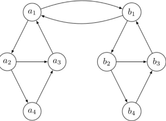
We now provide an example illustrating the relevance of the selection problem. Figure 2 il-lustrates an instance where the presence of restrictions that are inherent to recourse schemes has a negative impact on the expected number of transplants that can be realized. Assume that the maximum allowable cycle length is K = 4, that no chains are allowed, and that the success probability for each arc is equal to p = 0.5. If the maximum size of a relevant sub-set is equal to 4, the optimal solution is to test all arcs in the subgraph induced by the ver-tices {a1, a2, a3, a4} and all arcs in the subgraph induced by the vertices {b1, b2, b3, b4}. This
requires testing 10 arcs and leads to an expected 1.0625 transplants. However, testing the 8 arcs (a1, a2), (a2, a3), (a3, a1), (b1, b2), (b2, b3), (b3, b1)(a1, b1) and (b1, a1) leads to an expected 1.1328
transplants. a1 a2 a3 a4 b1 b2 b3 b4
Figure 2: An instance of the selection problem with K = 4, p = 0.5
3.1
An integer programming model for the selection problem
In the sequel, we often only use the index s to denote a scenario As, and we write s ∈ S instead
of As∈ S.
In order to model the selection problem, we introduce binary variables βi,j, for each arc (i, j) ∈
A, with the interpretation that βi,j = 1 if and only if (i, j) is selected in Stage 1 to undergo a
crossmatch test. The binary variables αc,s and δh,s are used to express the KEP that arises in
Stage 2: αc,s= 1 iff cycle c is selected when scenario Asarises, and δh,s= 1 iff chain h is selected.
Cs(Hs)is the set of cycles (chains)(possibly restricted in length, if the exchange program imposes
it) in the graph Gs= (V, As), and wc (wh) is the length of cycle c (chain h).
We can now write the following integer programming model for the selection problem: maxX s∈S qs( X c∈Cs wcαc,s+ X h∈Hs whδh,s) (7) Subject to X (i,j)∈A βi,j ≤ B (8)
αc,s− βi,j≤ 0 ∀s ∈ S, ∀c ∈ Cs, ∀(i, j) ∈ A(c), (9)
δh,s− βi,j≤ 0 ∀s ∈ S, ∀h ∈ Hs, ∀(i, j) ∈ A(h), (10)
X c∈Cs:v∈V (c) αc,s+ X h∈Hs:v∈V (h) δh,s≤ 1 ∀s ∈ S, ∀v ∈ V, (11) αc,s, δh,s ∈ {0, 1} ∀s ∈ S, ∀c ∈ Cs, h ∈ Hs, (12) βi,j∈ {0, 1} ∀(i, j) ∈ A. (13)
Constraint (8) ensures that at most B arcs are put to a crossmatch test. Next, constraints (9) link the selection of arcs to the choice of transplant cycles in each scenario: namely, a cycle can
only be chosen if all arcs that are part of this cycle have been tested. Finally, constraints (11) are the constraints from the deterministic KEP, which ensure that in each scenario, a patient-donor pair is assigned to at most one exchange.
Note that formulation (7)-(13) consists of a constraint upperbounding the number of arcs to be selected for crossmatch tests, constraints modeling the kidney exchange problem for each scenario, and constraints linking these two parts. In the above formulation, we chose to use constraints (11) from the cycle+chain formulation of the kidney exchange problem; it is important to realize that in fact this part could be replaced by any other valid formulation of KEP, and still arrive at a valid formulation of the selection problem.
3.2
The selection problem for a limited number of scenarios
Computationally, the selection problem poses challenges compared to the recourse models dis-cussed in Section 2.2. In particular, in the recourse schemes, all relevant cycles c or subsets T can be explicitly generated if their sizes are sufficiently small. Moreover, the computation of the coefficients wc or wT (expected number of transplants in a subgraph induced by a cycle c or a
subset T ) is facilitated by the fact that the subgraphs under consideration are small (see Pedroso [2014] and Klimentova et al. [2016]). This is no longer the case in model (7)-(13), where the variables βi,jcan generate arbitrary subgraphs, and where we have to take into account |S| = 2|A|
different scenarios.
In order to obtain a tractable model, therefore, we restrict our attention to a randomly gen-erated sample of the scenarios. More precisely, for any subset of scenarios S ⊆ S, we consider the variant of (7)-(13) where each occurrence of the set S is replaced by S. This yields an integer program of size polynomial in |V |, in |S|, and in the number of cycles of length at most K, which is O(|V |K) for fixed K. The optimal objective function value of the resulting selection problem
can be smaller than the “true” optimal value of the selection problem, since some scenarios have been discarded; however, we expect that it still provides a good approximation when S is large enough. Clearly, if we scale all qs so that Ps∈Sqs = 1, then the optimal value of the resulting
selection problem is nothing but the expected number of transplants over the restricted universe of scenarios S. In any case, it is important to understand that any set of values of the βij variables
satisfying constraint (9) provides a feasible solution of the selection problem and hence, can be implemented in practice.
3.3
The complexity of the selection problem
The computational complexity of the selection problem does not follow from the complexity of the classical kidney exchange problem. Indeed, whereas the KEP is polynomially solvable for K = 2, we prove that the selection problem is NP-hard, even for cycles of length at most K = 2.
Theorem 3.1. The selection problem is NP-hard, even for K = 2. Proof. See Appendix.
4
Solution Methods for the Selection Problem based on
Benders decomposition
The three formulations of the KEP mentioned in the previous section (Cycle+Chain, Extended Edge and Position-Indexed Edge Formulation) all have tight linear relaxations (Dickerson et al. [2016]). This suggests that relaxing the integrality of the scenario variables is likely to have little impact on the final solution. Since the vast majority of variables in any formulation of the selection problem are scenario variables, relaxing them decreases the number of binary variables by an order of magnitude. Moreover, if the scenario variables are no longer required to be binary, Benders decomposition becomes possible. Using Benders decomposition, formulation (7)-(13) can be reformulated as follows.
maxX s∈S qszs(β) (14) Subject to X (i,j)∈A β(i,j) ≤ B, (15) β(i,j) ∈ {0, 1}, (16)
with zs(β) the value of the optimal solution to the following problem:
maxX c∈Cs wcαc,s (17) Subject to X c∈Cs:(i,j)∈A(c) αc,s ≤ βi,j ∀(i, j) ∈ A, (18) X c∈Cs:v∈V (c) αc,s ≤ 1 ∀v ∈ V, (19) αc,s ≥ 0 ∀c ∈ Cs. (20)
The main idea behind Benders decomposition is to decouple the problem (14)-(16) from the subproblems (17)-(20); we omit further details for brevity.
4.1
Formulation strengthening
In an optimal solution to the selection problem, each selected arc is part of a cycle of length K or less, or a chain of length L or less. This is a natural result of the fact that in a subproblem, arcs can only be used for transplants if they are a part of a cycle for which every arc is tested and successful, or part of a chain with all preceding arcs successful. Tested arcs that are not part of a cycle or chain can thus not add any value to the objective. By decomposing the problem, this information is lost to the master problem. We add additional constraints to force the testing of arcs as part of a cycle or chain. In this way, the solutions to the restricted master will resemble realistic solutions to the full problem, even in early iterations of the generation of Benders’ cuts. We omit the exact formulation for brevity.
5
Computational Experiments
In this section, we discuss the results of the various solution approaches and formulations of the selection problem introduced in the previous sections. We first describe the experimental setting in Section 5.1. Then we compare in Section 5.2 the quality of the solutions found by solving the selection problem with the quality of the solutions found by recourse models. Next, in Section 5.3, we examine the computational efficiency of various approaches.
5.1
Experimental Setting
For these experiments, we generated kidney exchange graphs using the generator described by Saidman et al. [2006]. We consider three different sizes of graph, consisting of 25 patient-donor pairs, 50 patient-donor pairs and 25 patient-donor pairs plus one altruistic donor. For each of these sizes, we generate 40 graphs, divided into four groups of 10 graphs, with vertex failure rates of 20%, 40%, 60% and 80% respectively. These graphs form the basis of all instances. To complete the instances, we still have to specify an upper bound on the number of selected arcs B. In order to be able to compare our outcomes with those of the recourse models, we set B equal to the number of arcs that were tested in a solution found by using subset recourse on the same graph for a similar configuration. Specifically, the upper bound for an instance of the selection problem
with maximum cycle length K, is equal to the number of arcs tested in the optimal subset recourse solution with cycle length K and with maximum subset size 4. Finally, all instances are tested by including either S = 50, or 100, or 250, or 500 random scenarios in the formulation of the selection problem (see Section 3.2). To better compare computation times and solution quality between different solution approaches, each approach uses the exact same scenario set.
We distinguish four solution approaches:
1. BC-IP : Solution by branch-and-cut of a pure integer programming formulation (restricted to a subset S of scenarios).
2. BC-MIP : Solution by branch-and-cut of a mixed-integer formulation obtained by relaxing the scenario variables.
3. BD-MIP : Solution by Benders decomposition of a mixed-integer formulation obtained by relaxing the scenario variables.
4. BD-MIP+ : Solution by Benders decomposition of a mixed-integer formulation obtained by relaxing the scenario variables and adding additional constraints to enforce all selected arcs are part of a cycle or chain.
For each approach, the corresponding model is solved using CPLEX 12.8. For the two Benders-based approaches, we rely on CPLEX’s built-in Benders functionality. All instances were run with a time limit of 2 hours on 4 SandyBridge 2.6Ghz CPUs with 8Gb of memory.
5.2
Solution quality
Here, we compare the quality of the solutions found by solving the selection problem with the quality of the solutions found by solving the recourse models, as described in Section 2.2.
Max cycle length K ≤ 2 K ≤ 3 K ≤ 4 K ≤ 3 + Chains
Internal recourse 0.2 1.004 1.034 1.018 0.4 1.027 1.047 1.049 0.6 1.058 1.076 1.091 0.8 1.123 1.124 1.115 Subset recourse 0.2 1.011 1.019 1.013 1.018 0.4 1.016 1.010 1.012 1.016 0.6 1.038 1.029 1.021 1.022 0.8 1.021 1.048 1.048 1.028
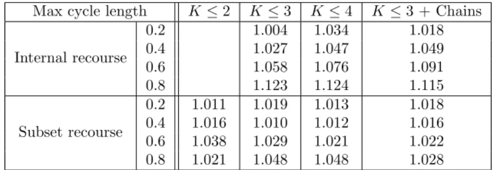
Table 1: Ratio of expected number of transplants from selection solutions over expected number of transplants from internal or subset recourse solutions. (BD-MIP, 500 scenarios,N = 25).
The results in Table 1 provide a measure of the increase in expected number of transplants achieved by the selection model, while using the same number of crossmatch tests as was used in the recourse models. We see that the improvement achieved by the solutions of the selection model depends both on the respective recourse model and on the failure rate. Indeed, as the failure rate goes up, the improvement gets larger with respect to both recourse models. Especially when compared with internal recourse, the selection model brings significant improvements - ranging up to 12% - at 60 and 80% failure rates. A closer look at the solutions suggests that this is mostly due to the inability of internal recourse to use overlapping 2-cycles which, at high failure rates, provide many more expected transplants per tested arc than longer cycles.
Incidentally, the results in Table 1 confirm that the restriction placed on the number of scenarios and the continuous relaxation of the scenario variables do not deteriorate the solution quality to an unacceptable degree: indeed, the solutions of the selection problem produced under these relaxations are still of higher quality than the solutions of the recourse models.
5.3
Computational Efficiency
In this section, we focus on the computational efficiency of different solution approaches when applied to the problem formulations.
In an initial experiment, we compare the three formulations for all four solution methods, on graphs with 25 nodes and maximum cycle length 3 (Section 5.3.1). In a next experiment, we investigate the impact of the maximum cycle length, by comparing the computation times needed for solving instances with maximum cycle lengths 2, 3 and 4 (Section 5.3.2). In our final set of experiments, we include chains, and look at computation times on graphs with 25+1 nodes (Section 5.3.3).
5.3.1 Solution Approach and KEP Formulation
In this experiment, we solve each instance by using each of the three formulations (cycle+chain, PIEF and EE), in each of the four solution approaches (BC-IP, BC-MIP, BD-MIP, BD-MIP+). Thus, each instance is solved 12 times. For reasons of brevity however, we only report in Table 2 the results for the PIEF-formulation; results for the cycle+chain formulation are comparable, while results for the EE formulation are worse.
Fail prob # Scen BC-IP BC-MIP BD-MIP BD-MIP+
0.2 50 15 22 518 33 100 23 23 510 18 250 149 314 1124* 91 500 814* 815* 1761* 232 0.4 50 12 13 14 8 100 14 16 18 41 250 37 48 761 45 500 154 156 1073 58 0.6 50 11 14 14 10 100 11 12 12 13 250 19 21 42 37 500 31 31 172 36 0.8 50 1.6 4.8 3.0 3.6 100 2.8 8.4 5.8 5.3 250 10 10 8.6 7.4 500 13 17 10 9.2
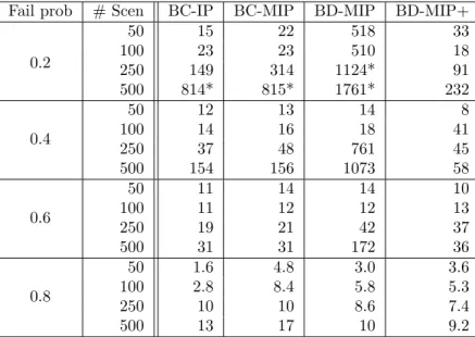
Table 2: Average computation times (in seconds) over 10 instances of the PIEF formulation for each solution method. N = 25, cycle length K ≤ 3. Asterisks denote some instances did not finish within 2 hours.
It appears from the results in Table 2 that BD-MIP+ (relaxing the scenario variables, applying Benders decomposition and enforcing cycles and chains are tested) generally leads to the lowest computation times, especially for harder instances involving a large number of scenarios or a small failure probability. We also note that adding these constraints significantly improves the performance of Benders decomposition (BD-MIP). If these constraints are not used, applying Benders decomposition is generally much slower than solving the integer programming version of the problem by branch-and-cut (BC-IP).
5.3.2 Cycle Length
In our next set of experiments, we use the PIEF formulation to solve the selection problem for instances with different maximum cycle lengths. Specifically, we look at formulations with cycle length limited to either 2, or 3, or 4 (these are the most commonly occurring maximum cycle lengths in real-life kidney exchanges). We restrict ourselves to sketching our main finding: increasing the
maximum cycle length has a strong influence on the total computation time. For a maximum cycle length of K = 2, no instance took more than half a minute, even with low failure rates and 500 scenarios. For cycle length K = 4 however, some of these instances could no longer be solved within 2 hours, even with BD-MIP+. Average computation times for 500 scenarios and 40% failure rates increase from around 70 seconds on average (K = 3) to 936 seconds (K = 4).
5.3.3 Chains
We have also looked at the impact of an altruist donor (NDD) and of the admissibility of chains on computation times.
Number of Scenarios Fail prob Solution Method 50 100 250 500
0.2 BC-IP 106.2 196.1 2389* 4385* BD-MIP 68.7 285 1886* 3283* BD-MIP+ 57.3 122.3 1748* 3296* 0.4 BC-IP 1033.7 2621* 4354* 4409* BD-MIP 1138 2080* 3379* 4756* BD-MIP+ 774 2976* 3853* 4058* 0.6 BC-IP 9.6 13.7 451* 785* BD-MIP 17.8 20.3 438* 739* BD-MIP+ 28.1 21.3 742* 781* 0.8 BC-IP 1.3 1.1 12.4 15.7 BD-MIP 1.0 1.1 9.5 13.4 BD-MIP+ 0.3 2.4 8.4 11.2
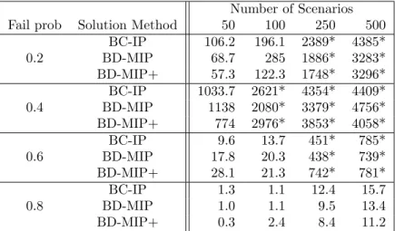
Table 3: Average computation time for different solution methods. N = 25 + 1 altruist. Cycle length K ≤ 3, chain length ≤ 3. Asterisks denote that some instances did not finish within 2 hours.
Table 3 shows that adding chains has a significant impact on computation times. Without an altruistic donor, most instances with cycle length 3 and 20% failure rate can be solved within 2 hours, even with 500 scenarios. In contrast, the addition of a single altruistic donor results in many instances that no longer can be solved within 2 hours. For the 20% and 40% failure rates, 8 out of 20 instances with 500 scenarios failed to finish, and 5 out of 20 for 250 scenarios. The density of the graph, and as a consequence, the upper bound on the number of selected arcs derived from the subset recourse solution, does play an important role. While 4 out of 10 instances with 20% failure rate and 500 scenarios failed to finish in 2 hours, 3 of these instances finished in under 20 seconds. These two groups of instances contain 182 and 122 arcs on average, respectively. The difficulty of the 40% instances is also apparently increasing with the density of the graphs for these instances.
5.3.4 Larger Datasets
In a final set of experiments, we ran BD-MIP+ on graphs of size 50. These graphs proved too large to solve within the time limit for the majority of instances. For 20% failure rates, 6 out of 10 failed to solve within the time limit, even for 50 scenarios. For 40% and 60% failure rates, this number was 6 and 5 respectively. The 80% failure rate instances on the other hand proved feasible, with only 2 out of 10 instances failing to finish for 500 scenarios, and only 1 out of 10 for 100 and 250 scenarios.
6
Conclusion
Selecting the right patient-donor pairs (that are potentially selected for a transplant) for cross-matching is a challenge. We have formulated the resulting problem as a two stage stochastic optimization problem, and we showed how Benders decomposition can help finding solutions to this challenge. The solutions we find in this way compare favorably with the solutions that are found using recourse models (which are based on identifying (small) subgraphs, whose arcs should then be selected for crossmatch tests). We have experimented extensively with different imple-mentations of solving the selection problem, and concluded that BD-MIP+ tends to give solutions faster than the other implementations. It also turns out that increasing the maximum cycle length, as well as allowing chains, has a strong negative impact on the running times.
References
David J Abraham, Avrim Blum, and Tuomas Sandholm. Clearing algorithms for barter exchange markets: Enabling nationwide kidney exchanges. In Proceedings of the 8th ACM conference on Electronic commerce, pages 295–304. ACM, 2007.
Sepehr Assadi, Sanjeev Khanna, and Yang Li. The stochastic matching problem with (very) few queries. In Proceedings of the 2016 ACM Conference on Economics and Computation, pages 43–60. ACM, 2016.
P. Bir´o, B. Haase-Kromwijk, T. Andersson, E. ´Asgeirsson, T. Baltesov´a, I. Boletis, C. Bolotinha, G. Bond, G. B¨ohmig, L. Burnapp, et al. Building kidney exchange programmes in europe–an overview of exchange practice and activities. Transplantation, 2018.
Avrim Blum, John P Dickerson, Nika Haghtalab, Ariel D Procaccia, Tuomas Sandholm, and Ankit Sharma. Ignorance is almost bliss: Near-optimal stochastic matching with few queries. In Proceedings of the Sixteenth ACM Conference on Economics and Computation, pages 325–342. ACM, 2015.
John P Dickerson, Ariel D Procaccia, and Tuomas Sandholm. Failure-aware kidney exchange. In Proceedings of the fourteenth ACM conference on Electronic commerce, pages 323–340. ACM, 2013.
John P Dickerson, David F Manlove, Benjamin Plaut, Tuomas Sandholm, and James Trimble. Position-indexed formulations for kidney exchange. In Proceedings of the 2016 ACM Conference on Economics and Computation, pages 25–42. ACM, 2016.
John P Dickerson, Ariel D Procaccia, and Tuomas Sandholm. Failure-aware kidney exchange. Management Science, 2018.
Sommer E Gentry, Robert A Montgomery, and Dorry L Segev. Kidney paired donation: fun-damentals, limitations, and expansions. American Journal of Kidney Diseases, 57(1):144–151, 2011.
Xenia Klimentova, Jo˜ao Pedro Pedroso, and Ana Viana. Maximising expectation of the number of transplants in kidney exchange programmes. Computers & Operations Research, 73:1–11, 2016. Vicky Mak-Hau. On the kidney exchange problem: cardinality constrained cycle and chain prob-lems on directed graphs: a survey of integer programming approaches. Journal of Combinatorial Optimization, 33(1):35–59, 2017.
David F Manlove and Gregg Omalley. Paired and altruistic kidney donation in the uk: Algorithms and experimentation. Journal of Experimental Algorithmics (JEA), 19:2–6, 2015.
Robert A Montgomery, Sommer E Gentry, William H Marks, Daniel S Warren, Janet Hiller, Julie Houp, Andrea A Zachary, J Keith Melancon, Warren R Maley, Hamid Rabb, et al. Domino paired kidney donation: a strategy to make best use of live non-directed donation. The Lancet, 368(9533):419–421, 2006.
NHS. Annual report on living donor kidney transplantation. Technical report, NHS, 2017a. NHS. Living donor kidney matching run process. Technical report, NHS, https://nhsbtdbe.
blob.core.windows.net/umbraco-assets-corp/2287/ldkmr-matching-process.pdf, 2017b. Retrieved 26 April 2018.
Joao Pedro Pedroso. Maximizing expectation on vertex-disjoint cycle packing. In International Conference on Computational Science and Its Applications, pages 32–46. Springer, 2014. Alvin E Roth, Tayfun S¨onmez, and M Utku ¨Unver. Kidney exchange. The Quarterly Journal of
Economics, 119(2):457–488, 2004.
Alvin E Roth, Tayfun S¨onmez, M Utku ¨Unver, Francis L Delmonico, and Susan L Saidman. Uti-lizing list exchange and nondirected donation through chainpaired kidney donations. American Journal of transplantation, 6(11):2694–2705, 2006.
Susan L Saidman, Alvin E Roth, Tayfun S¨onmez, M Utku ¨Unver, and Francis L Delmonico. Increasing the opportunity of live kidney donation by matching for two-and three-way exchanges. Transplantation, 81(5):773–782, 2006.
Appendix: The proof of Theorem 3.1
We first repeat the description of the input of the decision version of the selection problem.
Problem: The Decision version of the Selection Problem (DSP)
Instance: A simple, directed graph G = (V, A), a collection of m arc sets Ai ⊆ A (1 ≤ i ≤ m), numbers
K, H, B and Z.
Question: Does there exist an arc set A∗⊆ A such that |A∗| ≤ B and Pm
i=1
zK,H(V, A
i∩ A∗) ≥ Z ?
Recall that zK,H(G) stands for the optimum value of an instance of the KEP that is specified
by the graph G, and numbers K and H representing the maximum allowable cycle length and chain length, respectively. Observe that the last inequality in the question phrased above implicitly assumes that all scenario’s are equally likely, i.e, each scenario has a probability of m1 of actually occurring.
In the sequel we will restrict ourselves to instances with K = 2 without altruists, i.e., only 2-cycles are allowed. Thus, we can remove the superscripts in zK,H, and use z(G) to denote the
optimum solution value of such an instance specified by the graph G.
We will show that DSP is NP-Complete using a reduction from Satisfiability (SAT ). Recall that an instance of SAT is defined as follows.
Problem: SAT
Instance: A set of n0 variables {w
1, . . . , wn0} and a set of m0 clauses C = {c1, . . . , cm0} over the
variables.
Question: Is there a truth-assignment that satisfies all clauses in C? We rephrase Theorem 3.1 as follows.
Theorem 6.1. DSP is NP-complete, even forK = 2.
Proof. Given an instance of SAT , we construct an instance of DSP as follows. Let us first build the graph G = (V, A). The vertex set V is constructed as follows. For each clause ci ∈ C there
is a vertex vci ∈ V (i = 1, . . . , m), and for each variable wj there are three vertices in V , namely:
vwj, v
+ wj and v
−
wj (for j = 1, . . . , n). This describes V ; notice that V has 3n
0+ m0 vertices.
In our construction of the graph G, further detailed below, we use undirected edges. Each undirected edge between two vertices x, y ∈ V (denoted by e(x, y)) stands for two arcs, one from vertex x to vertex y, and one from vertex y to vertex x; thus, each edge in G stands for a 2-cycle. We now specify the arc sets Ai (1 ≤ i ≤ m), as well as the set A.
We set m = m0, i.e., there is an arc set A
i for every clause ci. The following set of edges is
present in each set Ai:
P ≡ {e(vwj, v
+
wj), e(vwj, v
−
wj), j = 1, . . . , n}.
In addition, consider for each clause ci (1 ≤ i ≤ m), and for each variable wj occurring
positively in clause ci, the edge set:
Pi+≡ ∪je(vci, v
+
wj) for i = 1, . . . , m.
Analogously, consider for each clause ci (1 ≤ i ≤ m), and for each variable wj occurring
negatively in clause ci, the edge set:
Pi−≡ ∪je(vci, v
−
wj) for i = 1, . . . , m.
We now define, for each i = 1, . . . , m:
Ai≡ P ∪ Pi+∪ P − i .
Moreover, we set A = ∪iAi. Further, we set B = 2(n + m) and Z = 2m(n + 1). This completes
the description of an instance of DSP.
We claim that there exists a satisfying truth assignment for C if and only if there exists an arc set A∗⊆ A with Pm
i=1
z(V, Ai∩ A∗) ≥ 2m(n + 1).
⇒ Suppose we have a satisfying truth-assignment for C. We will show how to identify an arc set A∗ such that whatever scenario/arc set A
i realizes, at least n + 1 edges (that is, 2(n + 1) arcs)
can be selected in an optimum solution of the resulting KEP, i.e., z(V, Ai∩ A∗) ≥ 2(n + 1).
If, in a satisfying truth assignment for C, variable wj is TRUE, we add edge e(vwj, v
+ wj) to
A∗; else we add edge e(v wj, v
− wj) to A
∗, j = 1, . . . , n. Further, since C is satisfiable, there exists
for each clause ci, a variable, say wj, whose truth assignment realizes this clause. Without loss
of generality, assume that wj occurs positively in ci; then we add edge e(vci, v
+ wj) to A
∗ for each
i = 1, . . . , m.
We have now specified A∗; observe that it contains n + m edges (or 2(n + m) = B arcs).
Consider now the instance of the KEP defined by the graph (V, Ai ∩ A∗). No matter which
particular arc set Ai is present, one can always find m + 1 pairwise non-adjacent edges. Indeed,
there are m edges present in P ∩ A∗, and, by construction of A∗, there is one edge incident to v ci
that is in A∗, and is not adjacent to any of the edges in P ∩ A∗. Hence z(V, A
i∩ A∗) ≥ m + 1 for
each i = 1, . . . , m, and this implies the instance of DSP is a yes-instance.
⇐ Now, we show that if the instance of DSP is a yes-instance, there must be a satisfying truth assignment for C. Consider the graph Gi= (V, Ai) (1 ≤ i ≤ m). We claim:
z(Gi) ≤ 2(n + 1) for i = 1, . . . , m. (21)
Indeed, in an optimum solution to the KEP instance defined by Gi, one can select at most one
edge out of the two adjacent edges {e(wj, w+j), e(wj, w−j)} for j = 1, . . . , n, and one can select
one edge incident to node vci. Since no other edges exist in Ai, the upper bound in (21) is valid.
Further, given that our instance of DSP is a yes-instance, we have:
m
X
i=1
z(V, Ai∩ A∗) ≥ 2m(n + 1). (22)
Combining (21) and (22) implies that A∗ is such that, for each i = 1, . . . , m, z(V, A
i∩ A∗) =
2(n + 1). Clearly, this value can only be realized by having in A∗ one edge out of each of the
n pairs {e(wj, w+j), e(wj, wj−)} (1 ≤ j ≤ n; the first n edges), and one edge incident to each vci
(1 ≤ i ≤ m; the last m edges). These first n edges in A∗ determine the truth assignment of the
variables: if e(wj, wj+) is in A∗, then we set wj to FALSE, else we set wj to TRUE. The last m
edges in A∗ imply that this truth assignment satisfies C: for each individual clause c
i there is an
edge e(vci, vwj) in A
∗, meaning there is a variable w