Joint optimization of monitoring quality and replacement decisions in condition-based maintenance

O

pen

A

rchive

T

oulouse

A

rchive

O

uverte

(OATAO)

OATAO is an open access repository that collects the work of some Toulouse

researchers and makes it freely available over the web where possible.

This is

an author's

version published in:

https://oatao.univ-toulouse.fr/23797

Official URL : https://doi.org/10.1016/j.ress.2019.04.034

To cite this version :

Any correspondence concerning this service should be sent to the repository administrator:

tech-oatao@listes-diff.inp-toulouse.fr

Nguyen, Thi Phuong Khanh and Do, Phuc and Huynh, Khac Tuan and Bérenguer,

Christophe and Grall, Antoine Joint optimization of monitoring quality and replacement

decisions in condition-based maintenance. (2019) Reliability Engineering and System Safety,

189. 177-195. ISSN 0951-8320

OATAO

Joint optimization of monitoring quality and replacement decisions in

condition-based maintenance

Khanh T. P. Nguyen

⁎,a

, Phuc Do

b

, Khac Tuan Huynh

c

, Christophe Bérenguer

d

, Antoine Grall

c

a_{Ecole Nationale d’Ingénieurs de Tarbes, INP Toulouse, LGP, France} b_{Univ. Lorraine,CRAN, UMR 7039, Vandoeuvre-les-Nancy, 54506, France} c_{Univ. Technology of Troyes, UMR 6281, ICD, ROSAS, LM2S, Troyes, France} d_{Univ. Grenoble Alpes, CNRS, Grenoble INP, GIPSA-lab, 38000 Grenoble, France}

A R T I C L E I N F O Keywords:

Condition Monitoring quality Condition Based Maintenance strategy Gamma process

Maintenance optimization Partially Observable Markov Decision Processes

A B S T R A C T

The quality of condition monitoring is an important factor affecting the effectiveness of a condition-based maintenance program. It depends closely on implemented inspection and instrument technologies, and even-tually on investment costs, i.e., a more accurate condition monitoring information requires a more sophisticated inspection, hence a higher cost. While numerous works in the literature have considered problems related to condition monitoring quality, (e.g., imperfect inspection models, detection and localization techniques, etc.) few of them focus on adjusting condition monitoring quality for condition-based maintenance optimization. In this paper, we investigate how such an adjustment can help to reduce the total cost of a condition-based maintenance program. The condition monitoring quality is characterized by the observation noises on the system degradation level returned by an inspection. A dynamic condition-based maintenance and inspection policy adapted to such a observation information is proposed and formulated based on Partially Observable Markov Decision Processes. The use and advantages of the proposed joint inspection and maintenance model are numerically discussed and compared to several inspection-maintenance policies through numerical examples.

1. Introduction

Condition monitoring (CM) is an important part in a condition based maintenance (CBM) program as it can provide useful information about the system state for maintenance decision making to improve the durability, reliability, and maintainability of industrial systems[13,28]. This leads to a steady growth of CBM optimization models in the lit erature which are more advanced and better adapted to practical in dustrial concerns. The performance of CBM policies with periodic in spections for single unit stochastic deteriorating systems has been investigated in[8,12,15]. Moreover, different studies aimed to optimize

the time interval between two successive inspections have been pre sented in the literature. In fact, it becomes more interesting to adapt the inspection interval according to the observed level of degradation state

[3,4] or according to the residual useful life (RUL) of the system

[5,9,30].

However, these above studies are based on the assumption of per fect condition monitoring which returns the real system state without errors. This assumption is not always verified in practical applications because, in spite of the progress of sensor technology and monitoring

techniques, the CM data are most often corrupted by noise and dis turbances. To deal with this problem, numerous works in the literature have been proposed. Newby and Barker in[20]considered an imperfect inspection model in which the observed deterioration state is subject to Gaussian error. Using Hidden Markov Model theory, Neves et al. studied in[19]how the model parameters estimated from imperfect observa tions can affect the optimization of CBM strategies. Ghasemi et al. in

[10]developed a partially observed Markov decision process (POMDP) to optimize the maintenance policy for a system whose state is hidden and can be estimated based on CM data. A continuous state POMDP coupled with a normalized unscented transform for non linear action models was proposed in [27]to formulate the problem of decision making for optimal management of civil structures. In[1], the authors presented an effective approach to solve MDP/POMDP problems for optimal sequential decision making in complex, large scale, non sta tionary, partially or fully observable stochastic engineering environ ments. For recent studies, the relation between the value of information and numerous key features of the monitoring system was investigated in[16]. In[18], the authors proposed a methodology for an integral risk based optimization of inspections in structural systems. The

⁎_{Corresponding author.}

E-mail addresses: nguyethipk85@gmail.com,tnguyen@enit.fr(K.T. . Nguyen). https://doi.org/10.1016/j.ress.2019.04.034

optimization problem is formulated based on a heuristic approach that is based on periodic inspection campaigns, a fixed repair criterion and does not consider the inspection quality adjustment options.

In reality, the quality of CM depends closely on the inspection and instrumentation technologies implemented, and ultimately on the costs invested. Therefore, its quality level could be controlled by adjusting inspection costs, i. e. paying higher costs to implement better mon itoring devices or to perform more thorough analysis of the deteriora tion, and to obtain more accurate CM information. The issue of

choosing between several kinds of inspection, or monitoring tools, at different costs, in order to adjust the inspection quality for a better decision making has been investigated in several works, e.g.

(6, 7,24,25). However, these works are mainly developed in a somehow different setting than the one considered in the present work: they consider that i) the system evolution follows intrinsically discrete states, and ii) the possible different inspections return the value of a discrete state, they have to be chosen within a finite predetermined set, and the observation probability matrix is fixed and known in advance for each of these inspections. In our setting, the system is basically subject to a continuous deterioration that is monitored by inspection, and this continuous state deteriorating system with continuous ob

servation is then mapped onto a discrete model for maintenance deci sion making ; the observation matrices are thus estimated at each de cision time and adapted to the actual deterioration and observation

characteristics of the system. As for the case of continuous observations

for a continuous degradation process, whose transition matrices can be

obtained through simulation, it has been already studied in (14). In

spired from these previous studies, the present work investigates the performance of a dynamic inspection maintenance policy for a system subject to a continuous degradation process. The quality of the de gradation information returned by inspections is characterized by the variance parameter of random errors following a Gaussian distribution,

(20). In (22), the authors developed a new flexible inspection strategy whose decision rules are adapted to this variance. It addresses the question of whether and when the adjustment of inspection quality from low level to high level is necessary, and underlines the value of CM quality adjustment in CBM optimization. This paper extends the work presented in (23), and develops two main original contributions: i) the proposition of a POMDP dynamic maintenance management framework based on continuous deterioration processes with imperfect monitoring, and ii) the in depth performance assessment of the pro posed framework and its in detail comparison with currently used CBM

approaches.

• Regarding the first contribution, this work proposes a discretization formulation for a continuous degradation process with random ob

servation noise, so that the POMDP decision framework can be de ployed and implemented starting from the continuous deterioration characteristics of the considered system. This approach allows to relax the requirement that the conditional probability of the discrete

observation given the system state is known and to connect more tightly the upper level maintenance decision process with the phy sical deterioration of the maintained system. In addition, the im perfect inspection quality characterized and modeled by an additive

observation noises is investigated and the resulting integrated im perfect inspection model, taking into account jointly the quality and the cost of an inspection, is also discussed. A comprehensive cost model including maintenance and inspection costs is then developed to evaluate the performance of the proposed joint CBM maintenance and monitoring policy.

• As for the second contribution, the behavior and the performance of

the proposed joint policy are numerically assessed and analyzed, and compared to currently used inspection and maintenance po licies. Sensitivity analyses regarding the performance of the pro posed policy are also investigated and discussed. Finally, the use and the advantages of the proposed models are illustrated and

highlighted.

The remainder of this paper is organized as follows. Section 2 de scribes the problem statement and its mathematical formulation.

Section 3 presents the proposed dynamic inspection maintenance policy. In addition, cost models and optimization processes are also discussed and formulated. Numerical experiments are presented in

Section 4. The proposed inspection maintenance policy is herein nu merically analyzed. Three variants of the proposed policy are also discussed to examine the performance of proposed general policy. Fi

nally, conclusions and future research directions are summarized in

Section 5.

2. Problem statement and mathematical formulation

2.1. Syswn description and asswnptions

Consider a single unit system subject to a stochastic continuous degradation process {XJ,., 0, X, E [R+ that evolves monotonically from the new state to the failed state in the absence of maintenance actions. The system fails when its degradation level exceeds a fixed failure threshold L, X, ;;:, L. The failure state is recognized without any in spection (i.e., self announcing failure). Let denote respectively Fx, and

fx, the cdf and the pdf of the degradation process {X,} at time t. The system degradation is often hidden, monitoring is then required to reveal the degradation level. "Continuous" monitoring, i.e. per formed at each time step (Ill), is usually very costly, and may be im possible to implement in some specific practical engineering applica tions (21). Note that Ill is nothing but the minimum time period at which the system can be accessed (and at which it could make sense to access it) for inspection. In practice, the value of Ill depends on both the monitoring system characteristics and the time behavior of the mon itored system. Depending on these, Ill can range form seconds (for fast evolving systems) to e.g. years ... (for slowly deteriorating systems). To make our modeling framework independent of this time scale, we take Ill equal to 1 (in arbitrary time units). In this framework, it is more suitable to implement periodic inspection whose length between two successive inspections T is a multiple of Ill (2). Then, at the beginning

of each observation period, if the system has failed, it is immediately replaced by a new one. Otherwise, an inspection is carried out to reveal the system state (degradation level) and then based on the obtained

information, the preventive maintenance decision can be made. How

ever, from a practical point of view, inspection operations may not reveal exactly the true system degradation state because of noise or

poor measurements. Accordingly, it is assumed that at each inspection time T,,, the observed state of the system, denoted Yr., can be described as

Yr.= Xr,,

+

•q,

where,

• Xr. is the true degradation level of the system at time Tn;

(1)

•

eq

is the measurement error and can be described by a random variable;

• q indicates the quality index of an inspection action.

It is assumed that the measurement errors are described by a Gaussian distribution N(O, <1f) with probability density function

2 1

l

(x)

Gu/x)

=

= e-i 'l'q

.

<1qv21r (2)

The standard deviation aq represents the inspection quality, i.e. an in spection with higher quality returns smaller variance of noise (20). In

that way, several inspection quality levels are herein investigated, e.g.,

exactly reveals the hidden system state. Note also that the inspection quality is usually increasing with the inspection cost, a quality based inspection model will be described in Section 3.2.

2.2. Probl.em statement of inspection quality adjustment and replacement decisions: an adaptive POMDP based decision model

For inspection and maintenance decision making, the crucial ques tions raising here are (i) whether or not investing in the improvement of

inspection quality to optimize the total maintenance cost, and (ii) how to adapt the maintenance decision to a given inspection quality. To answer to these questions, in this paper, a POMDP based inspection and maintenance model is proposed to optimize the total maintenance cost

over a planning horizon [O,

T,,.,J.

The POMDP framework has been widely used to model a sequential

decision process in which the system dynamics are characterized by a

Markov Decision Process, but whose underlying states cannot be di rectly observed. In detail, the POMDP is defined in discrete time and formally determined by a 7 tuple (Sz, A, Pr, C, So, Po, y), in which:

• Sz and

So

are respectively the sets of system discrete states and discrete observations. In order to apply the POMDP model for a single unit system subject to a stochastic continuous degradation process with Gaussian observation errors, it is necessary to dis cretize the system states and also their observation states. This step is presented in detail in Subsection 2.3. The probabilistic state transition law and conditional observation law are also derived in this section.

• A is the set of actions. For our problem, the set of actions A consists

of two subsets that are the inspection quality level options (q) and the maintenance options (Replace (R) or Do nothing (DN)). • Pr is the set of conditional transition probabilities between states. It

is derived in Subsection 2.3.1.

• C: Sz x A -+ IR is the cost function that is connected to the actions and the system states. Its formulation is presented in Subsections 3.2

and 3.3.

• PO is the set of conditional observation probabilities. In Subsection 2.3.2, the conditional observation probabilities are de rived.

• ye [O, 1) is the discount factor. In this paper, we are only interested in the expected sum of future cost and do not consider the dis counted value, so y

=

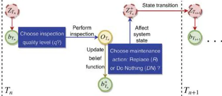
1.

Fig. 1 illustrates the POMDP based inspection and maintenance process. At the beginning of the decision period T,., if the system still works, the appropriate actions for system are investigated. Recall that the underlying discrete system state, noted Zr., is hidden: we only have the prior information about the probability distribution of the current state, called belief function

br ••

that is derived from the last period. To update the belief function at this moment, it is necessary to decide the inspection quality level (q) to perform an inspection. The details of the decision optimization (ie. how to choose an appropriate inspection) are

, , State transition .;, ,

,

zt.

t -- - - -..+tr".,I

~

Affect

Fig. 1. Illustration of POMDP-based inspection and maintenance process

presented in Section 3. Given an observation 01,,, the belief function is updated, see Subsection 2.4 for details. Then, the appropriate main tenance action is decided, see Section 3 for the details of the main tenance policy.

If

the DN option is chosen, the system state does not change. Contrarily, when the

R option

is chosen, the system is restored to its new state. Then, the corresponding belief function is derived for the next period, see Subsection 2.4 for the details of its transition process.

2.3. Stnte discretization modeling and formulati.on

The first step towards the development of a POMDP based modeling approach for maintenance evaluation purpose is the discretization of

the continuous time continuous state true deterioration process

{XJ,., 0 into continuous time discrete state process {Z,},., 0• This dis cretization step is not only required from a methodological point of

view for the model development, it is also interesting from a practical point of view. Indeed, very often in practice, even in the case of con

tinuously deteriorating items, the maintenance decision maker con siders only a few discrete deterioration states, such

as

:

"good", "minor deterioration", "medium deterioration", "severe deterioration", "cri tical deterioration", "failed". From a practical point of view, for the decision maker, considering only a few discrete deterioration states allows having a more synthetic view on the system state, and allows a simpler maintenance decision making process [29). In order to comply with this observed practice, in our proposed setting, we consider the number of discrete deterioration states N

as

an input for our modeling approach and for the policy optimisation, and not

as

a decision variable to be optimized.

The discrete state space of {Z,},., 0 is then defined by Sz

=

{l, 2, ... ,N, N

+

l}, where the state N

+

1 is the system failure state that corresponds to the interval [L, +oo) for the degradation level, and a state k e (1, 2, ... ,N} is a degradation state that corresponds to the in terval [(k - 1)1, kl), where I= ~

-The observed deterioration process {Yr.}11EN•

Yi;.

e IR, is then a dis

crete time continuous state stochastic process. Note that in practice the state space of {Y1,,}11E,., should be IR+, the theoretical state space IR ap

proaches the practical one when aq is not too large. As {X,},., 0, {Yr.lnEN

is also discretized in N

+

1 state

as

S0

= (1, 2, ...

,N, N

+

1} to obtain the discrete state observed deterioration process { OnlnEl'I• where the states 1

and N + 1 correspond to the intervals (-oo, [) and [L, +oo) respectively, and a state h e {2, ... ,N} corresponds to the interval [(h - 1)1, hi) with

I =

i

-

The process { Or,,}11E,., is thus a discrete time discrete state sto

chastic process. At an inspection time t

=

T., given the true deteriora tion level Zr,,

=

k, k e {l, ... ,N

+

l}, if the observed state On= k, then the system state is correctly detected; otherwise (i.e., On

=

h # k ), the detection is wrong. Fig. 2 shows an illustration of the system dete rioration modeling and discretization approach.

2.3.1. Derivation of the state transition law P(Z1n+i = mlZr. = k)

We derive in this section the expression of the state transition law P(Zrn+I = mlZr. = k), which is the conditional probability that the

N+l N 2 1 ~On N+l N

j

2

.

L

·----

~

-r

i

•

---

₀

x,

y7'

-_.,

-

•

-,

.

,

_I

_L

,

.

, ,

•

,,.

...

:

-

_I

·

-,X ___ c,c

I

-I

t

T2 Ts Ts

Fig. 2. Illustration of degradation-based failure model and discretization ap-proach

•

If1≤k=m≤N,

∫

= ∣ = = − < − − − − + + P Z k Z k P X X kl x f x dx F kl F k l ( ) ( ) ( ) ( ) (( 1) ) , T T k l kl T T X X X ( 1) n n n n Tn Tn Tn 1 1 (3)

•

If 1≤ k < m ≤ N,

∫

= ∣ = = − − ≤ − < − − − − + + P Z m Z k P m l x X X ml x f x dx F kl F k l ( ) (( 1) ) ( ) ( ) (( 1) ) , T T k l kl T T X X X ( 1) n n n n _Tn Tn Tn 1 1 (4)

•

If 1≤ k ≤ N,m=N+1,

∫

= + ∣ = = − ≥ − − − − + + P Z N Z k P X X L x f x dx F kl F k l ( 1 ) ( ) ( ) ( ) (( 1) ) , T T k l kl T T X X X ( 1) n n n n _Tn Tn Tn 1 1 (5)

•

Ifk=N+1,m=N+1, = + ∣ = + = ≤ ∣ ≤ = + + P Z( Tn 1 N 1ZTn N 1) P L( XTn 1L XTn) 1. (6)

The expressionsP Z( Tn+1=m Z∣ Tn=k)in the special case of a Gamma deterioration process are detailed in Appendix A.

2.3.2. Derivation of the conditional observation probability

= ∣ =

P Oq( n h ZTn k)

We derive in this section the expression of the conditional ob servation probability P Oq( n= ∣h ZTn=k) which is the conditional probability that the discrete observation is h given that the system is in the discrete state k (where h∈ SO and k∈ SZ), under an inspection

quality index q. Recall that Gσqis the cdf of the Gaussian noise and that

FXTnandfXTnare respectively the cumulative distribution function (cdf) and the probability density function (pdf) of the degradation process. To derive the expression of the conditional observation probability, the following cases have to be distinguished:

•

If h∈ [2, N] and k ∈ [1, N],

∫

= ∣ = = − − − − − − − P O h Z k G hl x G h l x f x dx F kl F k l ( ) ( ( ) (( 1) )) ( ) ( ) (( 1) ) , q n T k l kl σ σ X X X ( 1) n q q Tn Tn Tn (7)

•

Ifh=N+1 and k∈ [1, N],

∫

= + ∣ = = − − − − − P O N Z k G L x f x dx F kl F k l ( 1 ) (1 ( )) ( ) ( ) (( 1) ) , q n T k l kl σ X X X ( 1) n q _Tn Tn Tn (8)

•

If h∈ [2, N] and =k N+1,

∫

= ∣ = + = − − − − − ∞ P O h Z N G hl x G h l x f x dx F L ( 1) ( ( ) (( 1) )) ( ) 1 ( ) , q n T L σ σ X X n q q _Tn Tn (9)

•

Ifh=N+1 andk=N+1,

∫

= + ∣ = + = − − − ∞ P O N Z N G L x f x dx F L ( 1 1) (1 ( )) ( ) 1 ( ) , q n T L σ X X n q Tn Tn (10)

•

Ifh=1 andk∈[1,N+1],

∑

= ∣ = = − = ∣ = = + P Oq( n 1ZT k) 1 P O( h Z k). h N q n T 2 1 n n (11)

These different expressions ofP O( n= ∣h ZTn=k)are further detailed in Appendix B for the special case of a Gamma deterioration process.

The integrals inEqs. (3 11) are numerically evaluated using the Gauss Kronrod quadrature formula [11] implemented in the in tegrate R function.

2.4. Belief function

Since the real degradation state of system cannot be revealed ex actly by imperfect inspections, then the state of knowledge of the de cision maker on the system state at time t is characterized by a belief function btconsisting of a vector of the probabilities of the real system

degradation level over the discrete state spaceSZ. Each element of btis

defined asP Z( t=k),k∈ SZ. For a new system, the initial belief func

tion, noted b0 is known without inspection:b0=[1, 0, 0. ..0],i.e. the

probability of the new state is equal to 1 and the one of other states is 0. As the observation measure obtained after an inspection at Tnde

pends on the system state and the inspection quality index q, then =

P Oq( n h)the probability that the observation measure is h is given by:

∑

= = = = = ∈ P Oq( n h) P Z( k P O)· ( h Z| k) k T q n T SZ n n (12) Given the observation measureOn=hafter an inspection with quality index q, we update the belief functionbTn+whose each element is given

by: = = = = = = = = = + P Z k P Z k O h P Z k P O h Z k P O h ( ) ( | ) ( )· ( | ) ( ) T T n T q n T q n n n n n (13) where_{P Z(} +=_k)

Tn is the probability that the real degradation state is k given that the observation h is obtained after an inspection at quality index q. The value of the belief function at the next inspection period, without maintenance can then be evaluated as :

= + ′

+

bTn 1 bTn·T( | )z zn (14)

whereT( | )z zn′ is the state transition matrix of the discrete system state without maintenance action. Each element of the state transition ma trix, that is the conditional probability that the system is in the discrete state m at the inspection dateTn+1given that it is in the discrete state k

at the inspection date Tn, where k, m∈ SZand m≥ k, have been derived

inSubsection 2.3.1.

3. Dynamic inspection-maintenance policy

In this section, a dynamic inspection maintenance policy is pro posed. Within this policy, the maintenance decision for both inspection quality adjustment and preventive maintenance action is based on the knowledge on the system deterioration state summarized in the belief function vector. The maintenance cost is herein used as a criterion for the optimization process.

system is in the discrete state m at the inspection date Tn+1 given that it

is in the discrete state k at the inspection date Tn, where k, m ∈ SZ and m ≥ k. Recall that FXTnand fXTnare respectively the cdf and the pdf of the degradation process, the four following configurations of m and k are considered.

3.1. Policy description

At each periodic discrete timeTn=Tn−1+T(T is a decision variable which needs to be optimized), if the system is still functioning, the online adaption process for the inspection quality and the maintenance decision structure are as follows:

•

First, the belief function is derived from the information at the last period (see againSection 2.4). Then, an inspection quality index q is selected by minimizing the expected total maintenance cost corre sponding to the belief function value at this moment. It should be noticed that the relationship between the belief function and the expected maintenance cost is discussed inSection 3.3. An associated inspection costc_iq is incurred when performing an inspection with quality index q;

•

Given the deterioration state observation returned by the inspection operation, the belief function is then updated;

•

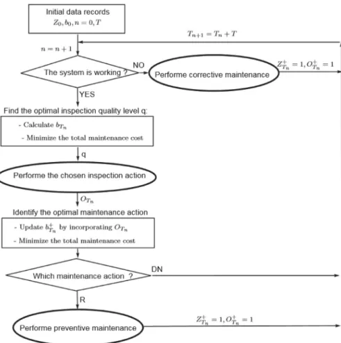
Based on the updated belief function after inspection, the preventive maintenance action (replace the system (R) or do nothing (DN)) is selected by minimizing the expected total maintenance cost.

Fig. 3 illustrates the decision process for inspection and main tenance decision making.

The proposed policy involves two kinds of decision variables:

•

The inspection period T: this is a global decision variable in the sense that it is set of the whole planning horizon.

•

Two local decision variables, whose value is set for each discrete time period (Tn=Tn−1+T): inspection quality index q and main tenance action (replacement R or DN).

Tofind the optimal value of these decision variables, cost models are herein developed and presented in next sections.

3.2. Inspection cost formulation

It is pointed out in the literature that a higher quality inspection incurs a higher inspection cost, see for instance [5]. Therefore, we consider σqas a decreasing function of the corresponding inspection

costciq. In that sense, it is assumed in this work that when the quality index q is chosen at inspection time Tn, one has to pay an inspection

cost which is defined as:

⎜ ⎟ = ⎛ ⎝ ⎜ −⎛ ⎝ ⎞ ⎠ − ⎞ ⎠ ⎟ c c ν σ σ ν · ·( 1) , iq il q l k (15) where

•

σlandcilare respectively the standard deviation of the measurement errors and the inspection cost at the lowest inspection quality;

•

ν is the ratio between the cost of the best quality inspection and the cost of the lowest quality inspection ( =ν cih/cil);

•

k is the parameter characterizing the shape of the inspection cost function.

Note that, for the best quality inspection, we suppose that the ob servation reveals the real system state,σq=0.

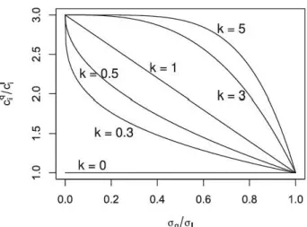
According to this cost model, different shapes of the inspection cost function can be found depending on the value of k, seeFig. 4 as an illustration:

•

k=0, the inspection cost is constant (ciq=cil)

•

0 < k < 1, the inspection cost is a convex function: the inspection

Fig. 3. Illustration of the proposed maintenance policy. Initial data records

Zo,bo,n

=

0, T

Find the optimal inspection quality level q: - Calculate b-r,.

-Minimize the total maintenance cost

Orn

Identify the optimal maintenance action

-Update bt by incorporating Orn

-Minimize the total maintenance cost

Tn+l =Tn +T

DN

0 M LO N -0 -0

---

\'Ii

"u

·

~

....

~ 0.0 0.2 0.4 0.6 0.8 1.0

Fig. 4. lliustration of inspection cost function, v

=

3

cost decreases more than the decrease gain of inspection quality

• k

=

1, the inspection cost is a linear function

•

k

> 1, the inspection cost is a concave function: the inspection cost

decreases less than the decrease gain of inspection quality.

3.3. Maintenance total cost formukJti.on and optimization

The optimal cost incurred by this policy is given by the minimal value of the expected cost t'(o,r,.d](T, b0) associated to different values of

inspection period length T :

v

f

=

minr(lio,r,nd](T, bo)), where

lio,T.,.d](T, bo) is calculated by :

i-[o,T.,.d](T, bo)

=

IE[Co(bo)) + "lfo,r,.d](T, br₁) (16) At the initial time, the system is new, then we do nothing. Therefore,

the system continuously operates until the first inspection at time T 1,

the belief function at this time is !mown as br₁ (calculated by Eq. (14)). Hence, the expected accumulated cost t'(o,r,.d](T, b0) over the planning period [0, T,,.il is the sum of the expected downtime cost IE[Co(bo))

during period [O, Ti.] and the expected accumulated cost from the ob

servation period T1 until the final time T ,n,1.

A replacement, whether preventive or corrective, can only be in stantaneously performed at inspection times. Therefore, there exists the possibility of system failure, and an additional cost is incurred from the failure time until the next replacement time with down time cost rate, ed. let IE[C0(Zr,,

=

k)) be the expected downtime cost of the system during the period [T,,, T,,+il when !mowing the real state Zr.

=

k at T,.,

then the expected downtime cost IE[C00 ) of the system during the

period [T., T,,+il when knowing the belief function br,, is given by:

IE[Co(br.)]

=

1:

P(Zi-.

=

k)·IE[C0(Zi-.

=

k)]

te:Sz (17)

where the evaluation of IE[Co(Zr.

=

k)] is made using a discretization

method. Recall that the length between two successive inspections T is a

multiple of 1!,,t-. T

=

J·ll.t, in order words, the interval [T,,, Yn+il can be

discretized into J sub interval of length M, that is [T., Tn+ll.t[,

[T,.

+

ll.t, Tn+2ll.t[, ... , and [T,.

+

(J - l)ll.t, Tn+il• If the failure time be

longs to one of these intervals, we approximate it by the left end value.

Given cd the downtime cost rate c,i, if the failure time belongs

[T,1

+

(j - l)ll.t, T,,+jll.t [, where (1 ~ j ~ J, j ERO then the downtime

cost associated is evaluated to

ca-CT;

-

(j - l)ll.t).

Hence, the expected downtime cost IE[C0(Z1,,

=

k)) during interval IT,,,

Yn

+

ii

is given by:

J

IE[Co(Zr.

=

k)]

=

ea

1:

(P(zr.+jllt

=

N

+

llZr.

j=I

=

k)

-

P(Zr,,+u-1)111

=

N

+

llZr.

=

k)('Ji - (j - l)ll.t) ₍₁₈₎

where P(Zr.+j111

=

N

+

llZr.

=

k) can be evaluated be Eq. (5)

let teJ be the maximal integer that is inferior

thane,

then we define

N

=

l

re;'

J

as the number of observation periods during [0, T,,.,J.

For 1 ~

n

~ N - 1, the expected accumulated cost from Tn until the

final time Tend is given by:

V,1(T, b1,,)

=

IPJ(Tn)CcO

+

(1 - IPj(T,1))·

min(c?

+

1:

Pq(On

=

h)·min[CRO, CoNO)) q hESo

(19) where IPj(t) is the probability that the system is failed at t In detail, the

equation Eq. (19) is evaluated by the sum of :

1. Cc(br •• T): the expected accumulated cost associated to system

failure at the beginning of the observation period T,., see Eq. (20).

Cc(br., T) is the sum between the corrective replacement cost Cc, the expected downtime cost IE[C0(br.)] during [Tn, Tn+il, and the ex pected accumulated cost from the next period until the end of the planning horizon V,,+1(T, br1).

2. The expected accumulated cost associated to the case where the

system still works at the beginning of the observation period Tn. In

this case, it is necessary to decide the quality level for inspection.

Then, based on the updated belief function, the adequate main

tenance action is performed (preventive replacement (R) or do

nothing (DN)). The quality index q is chosen such that the expected

cost associated to this decision (accumulated from this time until the

end of the planning horizon) is minimal It is evaluated using the

inspection cost

c?,

the minimal value of the expected accumulated

cost CR(·) corresponding to the preventive replacement decision

(see Eq. (21)) and the expected accumulated cost C0 N( ·) corre

sponding to the do nothing decision (see Eq. (22)).

• CR(·) is evaluated as the sum of the preventive replacement cost

cp,

the expected downtime cost IE[Co(bo)], and the expected ac

cumulated cost from the next period until the end of the planning horizon V,,+1 (T, br₁) (see Eq. (21)).

• C0 ~ ·) is evaluated as the sum of the expected downtime cost

IE[Co(br +)I during [T., Tn+1) and the expected accumulated cost

from th~ next period until the end of the planning horizon

V.+1 (T, b1ri+1) (see Eq. (22)).

CcO

=

Cc+ V,,+1(T, brn+i)

+ IE

[Co(bo)) (20)

(21)

(22)

For the terminal condition of the planning horizon, we suppose that

Vi~nd

=

0.

4. Numerical experiments

In this section, we present the results of a numerical experiment implemented to get a better insight into the behavior of the proposed inspection and maintenance policy. Through this example, the aim is to show how the proposed maintenance decision rule helps to choose whether and when it is necessary to improve the inspection quality, and

to illustrate the benefit of implementing a flexible/dynamic inspection

and maintenance policy instead of a static one.

For this example, the system degradation is assumed to follow a

homogeneous Gamma process, see Appendix A. The parameters (char

acteristics and costs of the system deterioration, inspection and main

Table 1.

In the remainder of this section, benchmark maintenance policies arefirst presented: they are used for performance comparison with the proposed maintenance policy. The behavior of the proposed main tenance policy, tuned at its optimum, is then analyzed and compared to the behavior of the benchmark policies. Finally, the benefit of using the proposed maintenance policy in terms of maintenance cost is in vestigated and compared to the cost performance of the benchmark policies.

4.1. Presentation of the benchmark policies for performance analysis and comparison

In order to study the performance of the proposed dynamic in spection maintenance policy (presented inSection 3), namely policy P, three variant policies (namely P1, P2 and P3) are considered:

•

Policy P1 - Classic CBM (Condition Based Maintenance) policy. System degradation states are periodically inspected after period length T. If the observed degradation state is greater than a pre ventive replacement threshold M, the system is then replaced by a new one. The inspection quality cannot be adjusted. Either a CBM with low quality inspections (notedPOl

1) or a CBM with high quality

inspections (noted POh

1) is considered in this experiment and ap

plied throughout a planning horizon [0, Tend].

•

Policy P2 - CBM with dynamic inspections policy. Similar to Policy P1, a CBM policy is applied based on the observed degrada tion state. The inspection quality can be adjusted at each period. In detail, at the beginning of an inspection period, we decide the quality index q for an instantaneous inspection with a costc_iq(de pending on the inspection quality q).

•

Policy P3 - Dynamic maintenance policy withfixed inspection quality. Similar to Policy1, the inspection quality cannot be ad justed: either a dynamic replacement policy with low quality in spections (notedPOl

3) or with high quality inspections (noted PO3h)

is applied throughout a planning horizon [0, Tend]. Given an ob

servation, the belief function is updated and then the relevant ex pected cost is evaluated for each option (DN or R). Based on the comparison between these costs, we decide to replace the system or not.

Table 2reports a summary of the proposed policy (policy P) and the variant policies considered for comparison (policy P1, P2 and P3).

The formulation of the cost model for the three policies P1, P2 and P3 can be adapted from the cost model developed for the proposed policy in Section 3.3. The detailed mathematical developments are presented in Appendix C. For each policy, the optimal expected accu mulated cost over a planning horizon is evaluated using the classical backward induction algorithm and the grid based algorithm[17]. For numerical examples, the system states and observations are discretized

and ∑_i=1ei=1

6

. For each value of T, using the backward induction al gorithm, the cost function corresponding to each possible maintenance action at Tendis computed for the set of points in the belief space. The

optimal action at this moment is the one leading to the minimal cost. Next, using the optimal cost function at Tn, we derive the cost function

corresponding to every action atTn−1for the belief space and thenfind

the optimal action. This procedure is iterated untiln=1, so that the optimal expected cost over the planning horizon is obtained.

Let VP 0 l 1_{and V}P 0 h

1 _{be respectively the minimal value of the optimal}

expected accumulated cost incurred by Policy P1 with either low quality inspection or high quality inspections:

=

VP min(VP,VP)

0 0 0

l h

1 1 1 ₍₂₃₎

Similarly, the optimal expected accumulated cost for Policy P3 is given by:

=

V0P min(V0P,V0P) l h

3 3 3 ₍₂₄₎

For policies with quality adjusted inspections (policies P and P2), six quality levels are examined. In details, the probability that an ob servation reveals the true system state is respectively 100%, 90%, 80%, 70%, 60% and 50% for these six inspection levels. Note that q is the quality index,q=1 characterizes the highest quality and q=6 re presents the lowest quality. At the initial moment, T0, the system is

totally new, therefore, its state is known and we are only interested in the maintenance options for next periods (from the thefirst inspection period, T1).

4.2. Discussion of the belief function deviation under an adjusted inspection quality policy

The initial prior belief is assumed to be perfect. In practice, this assumption is reasonable because, considering a new system, it is trivial to have a perfect prior knowledge:Z=1. In addition, at every stage, the belief function is updated according to the observation. Therefore, an adjusted inspection quality policy with the perfect inspection option allows correcting belief functions. Hence, the belief function does not derived so far from the truth. For an illustration,Fig. 5presents the changes of the belief function at the early stages of the policy appli cation in two cases: highest quality inspection and lowest quality in spection. Note that, inFig. 5, for a simplification of the notations, the

belief function bTnis represented by bn. We consider a system whose the

deterioration process is discretized by 6 statesZ=[1, 2, 3, ...6], with the failure stateZ=6. From the initial stateZ=1, after one decision period, the belief function is equal tob1=[0.63, 0.24, 0.09, 0.03, 0.01, 0]. Then, a highest quality inspection allows correcting the belief function thanks to its perfect outcome. Indeed, given the system state at thefirst stage, Z1=1, the updated belief function in the case of the highest

quality inspection,b1+in subfig. 6(a), provides the probability that the

system belongs to the initial state is 1,P Z( 1=1)=1. In the case of the lowest inspection, see subfig. 6(b), thanks to the correct result,O1=1, its relevant belief function indicates that the probability of the initial state is highP Z( 1=1)=0.9. One can notice that even if using the λ β L k cp cc cd Tend cil ν σl σh

1 1 5 1 50 100 25 30 1 3 0.67 0

Table 2

Overview of the 4 policies

Maintenance policy Inspection policy Decision variables

Policy P Dynamic Adjusted T set throughout the planning horizon, q at the beginning of each inspection period and action (R or DN) corresponding to the updated belief function

Policy P1 Fixed Fixed (T, M) set throughout the planning horizon

Policy P2 Fixed Adjusted (T, M) set throughout the planning horizon and q at the beginning of each inspection period

Policy P3 Dynamic Fixed T set throughout the planning horizon and action (R or DN) corresponding to the updated belief function at every inspection period

Table 1

Parameters _{set for the numerical example.}

by 6 states. Among them, ZTn= 6 is the failure state. Then, the belief space is discretized by a set of vectors of 6 elements ei. Each element of

Zo

=

1

; - - - . .

b,

=

[0.63,0.24,0.09,0.03,0.01,01 b,

=

(0.63,0.24,0.09,0.03,0.0l,OJ ] I

b

T

=

11.0.0.0.0.01

bT

= [0.9,0.1,0,0,0,0J 112

=

[0.4,0.38,0.14,0.05,0.02,0.011 ~ =2 b2 = [0.36.0.38,0.17,0.06.0.02,0.01)

b

t =

[0, 1,0,0,0,01

b

t

= [0.02,0.44,0.47,0.07,0,01 b3

=

[0,0.4,0.38,0.14,0.05,0.03) b3

=

[0.0l.0.18,0.35,0.27,0.12,0.07)

b

t =

(0, l,0,0,0,01

b

l

=

[0,0.13,0.66,0.2,0.0l.Ol b4

=

[0,0.4,0.38,0.14,0.05,0.03) b4

=

[0,0.05,0.31,0.35,0.18,0.IIJ

bt

= [0,0,0.02,0.38,0.48,0.12] bs

=

[0,0,0,0,0.39,0.61] bs

=

[0,0,0.0l,0.14,0.34,0.5)

(a.)

Highe

s

t qu

a

lity i

ns

pec

t

ion

,

q

=

I

(b

)

Lowe

st

qu

a

lity inspe

ct

ion

,

q

=

6

Fig. 5. lliustration of belief function changes at the early stages.

bn =[0.63, 0.24, 0.09. 0.Q3, 0.01, OJ

•

---

-

----:-

!

~.

~

_,

· ·

,

.

•

. . -

L.:....:..I

I ' I .

i

~ \

I • '

.

~-

--

-1 \\ ••

•

-lill'':g

-•

1-

- -

~--i

I \:\

\>.,

' ', ' ', ,

\

. .

•

.ll9!

,

a-

- -

-t-

--i

•

[

~J<_

Fig. 6. lliustration of the behavior of the optimally tuned policy P2 at steady

state

lowest inspection, the belief function is close to the ground truth thanks to the correct inspection result. Next, after consecutive wrong ob

servations, 02 = 03 = 3, the belief function deviates quite far from the

truth, for example at the beginning of the fourth decision period,

b4

=

(0, 0.05, 0.31, 0.35, 0.18, 0.11], instead of the correct results b4

=

(0, 0.4, 0.38, 0.14, 0.05, 0.03). However, thanks to the correct ob

servation 04

= 5,

the belief function is updated and then, its value at the

next period, i.e.

bs

= (0, 0, 0.01, 0.14, 0.35, 0.5

) does not deviate so far

from the ground truth, i.e.

bs

= (0, 0, 0, 0, 0.39, 0.61

).

4.3. Analysis of the optimally tuned

policies

In order to guarantee the solution accuracy, a large belief space is

considered, consequently the computational cost is high. Using the

MacBook Pro 3,1 GHz Intel Core i5, the computational time to optimize

the policies 1, 2, 3 and 4 are respectively 980, 8550, 1020 and 16890

seconds. Considering the set of parameters presented in Table 1, all the

considered policies are optimized and the following analysis can be

made on their optimal structure:

• For maintenance policies with non adjusted quality inspections (i.e.

Pl and P3),

• Policy Pl Under the optimal tuning of the decision variables,

lowest quality inspections are performed at every inspection

period T

= 1

and the system is preventively replaced when the

obse,ved

state is greater than 4,

Or.

>

4, which means that the

replacement threshold M is 5. In summary, the optimal decision

variables are q• = 6 and (T*, M*) = (1, 5).

• Policy P3 Highest quality inspections (q

=

1) are performed

every period T

= 2

and the replacement option triggered when the

degradation state is equal or greater than 4, Z.r,, ~ 4. Note that for

highest quality inspections, the observation reveals the true de

gradation state.

• For maintenance policies with adjusted quality inspections (i.e. P2

and P), the optimal action is decided by minimizing the relevant

expected cost function that depends on the action and belief func

(without the influence of the starting ending conditions) ; note that the steady state behavior is guaranteed when there are still at least 11 periods from the current decision period to the end of the planning horizon, Tend. As the belief function is strictly connected to

the observation state and the historical process of the maintenance actions, in order to facilitate the description of the optimal policy, we present it in the format of the action process and the observation state. The behavior of these two policies, when optimally tuned, is sketched inFigs. 6and7, and described below.

•

Policy P2 The system is inspected at every periodT=1and is preventively replaced when the observed state is greater than 4, i.e.( ,T M)=(1, 5). For an illustration, we assume that the belief

function at the decision period Tn is

=

bn [0.63, 0.24, 0.09, 0.03, 0.01, 0]. Then, the optimal stationary adjusted inspection quality policy in this case prescribes that at this inspection period, the lowest quality inspectionq=6 is im plemented, seeFig. 6. If the observation state O is lower than 3, the lowest quality inspection is still used at the inspection period

+

Tn 1. In the case of the observation stateO=3at Tn, the inspec

tion with quality indexq=3is performed at the next period,Tn+1,

while for the higher observation result,O=4, the system is in spected with higher inspection quality, q=2. For O > 4, the system will be replaced by a new one, thus, a new maintenance cycle is then repeatedly performed. Next, atTn+1,considerFig. 6,

wefind that the inspection quality is flexibly adjusted for every situation that depends on the historical action process and the observation gathered atTn+1. Note that considering the planning

horizonTend=30,the terminal condition impact is negligible for Tn,Tn+1andTn+2whenTn+2≤19.

•

Policy P Under the optimally tuned policy P, the system is in spected at every periodT=1. For an illustration, we assume that the belief function at the decision period Tn is

=

bn [0.63, 0.24, 0.09, 0.03, 0.01, 0]. Then, the optimal stationary policy in this case prescribes that at this inspection period, the lowest quality inspection q=6 is implemented. Based on the updated belief function corresponding to the observation state, the maintenance action is determined between DN (“Do Nothing”) or R (“Replace”). For example, see Fig. 7, if the ob served state at Tnis lower or equal to 4, O≤ 4, we do nothing

(DN) while the system is replaced (R) when O≥ 5. In the case of the observation stateO=1at Tn, without replacement the system

is inspected with lowest quality ( =q 6) at the next inspection periodTn+1and then is replaced for O≥ 5. If the observation state

at Tn is O=2 or 3, the inspection with quality q=3 is

implemented atTn+1and the system is replaced for O > 3.Fig. 7

shows a policy behavior under which both replacement option and the inspection quality areflexibly changed to adapt to every situation. Note that considering the planning horizonTend=30, the steady state is guaranteed for Tn,Tn+1andTn+2whenTn+2≤19.

4.4. Comparison of the policies performance in terms of cost

In this section, we study and compare the cost performance of the considered policies. To this aim, let consider the percentage of the difference in their optimal values defined as follows:

= − = − = − = − = − = − V V V V V V V V V V V V V V V V V V Δ ( )100%; Δ ( )100%; Δ ( )100%; Δ ( )100%; Δ ( )100%; Δ ( )100%; P P P P P P P P P P P P P P P P P P 12 0 0 0 13 0 0 0 14 0 0 0 23 0 0 0 24 0 0 0 34 0 0 0 2 1 1 3 1 1 1 1 3 2 2 2 2 3 3 (25) For example, Δ12 quantifies the relative cost increase (when

Δ12> 0) or decrease (when Δ12< 0) between the optimal costs of

Policy P2 and Policy P1. IfΔ12< 0, Policy P2 is more cost efficient than

Policy P1 since it incurs a lower cost over the considered planning horizon. The other Δij (i < j, 1≤ i ≤ 3 and 1 ≤ i ≤ 4) can be inter

preted in the same way.

4.4.1. Influence of the maintained system parameters on the relative performance of the maintenance policies

We investigate here the effect on the policies performance of the different characteristics of the maintained system (parameter char acterizing the shape of the inspection cost function k, inspection cost ci,

downtime cost rate cd, variance coefficient of the degradation process vc

and the ratio between corrective and preventive replacement cost cc/

cp). In order to compare the performance between the different in

spection maintenance policies, we consider only the difference (Δij) in

their optimal values.Table 3presents the Pearson correlation values, that belong to −[ 1, 1], between the system parameters and the relative cost difference Δij. This Pearson correlation is equal to zero when there

is no the correlation between two variables and equal to 1 (or 1) when two variables are positive (or negative) linearly proportional. The re sults presented inTable 3are obtained from a set of numerical ex periments with different values of k={0.1, 0.3, 1, 3, 5}, ci∈ [1, 5],

cd∈ [20, 35], vc ∈ [0.1, 0.7], and cc/cp∈ [1, 5].

The following conclusions can be drawn:

•

In general, the impact of the ratio between corrective and pre ventive maintenance cost cc/cpon the performance difference be

tween these inspection maintenance policies (Δij) is not significant.

•

The performance differences between adjusted quality inspections and non adjusted quality inspections, that are characterized by the Fig. 7. Illustration of the behavior of the Proposed Policy P at steady state,

when optimally tuned

Table 3

Pearson correlation between the parameters inputs and theΔij.k: parameter characterizing the shape of the inspection cost function, ci: inspection cost, cd: downtime cost rate, vc: variance coefficient of degradation process, and cc/cp: the ratio between corrective and preventive replacement cost

k ci cd vc cc/cp Policy P1 vs P2 (Δ12) 0.68 0.57 0 -0.03 0 Policy P1 vs P3 (Δ13) 0 0.89 -0.14 0.88 -0.11 Policy P1 vs P (Δ14) 0.52 0.76 -0.1 -0.69 -0.04 Policy P2 vs P3 (Δ23) -0.83 -0.07 -0.09 0.04 -0.01 Policy P2 vs P (Δ24) -0.12 0.81 -0.27 0.69 -0.1 Policy P3 vs P (Δ34) 0.78 0.48 -0.05 0.04 0 bn=[0.63, 0.24, 0.09, O.Q3, 0.01, OJ I ~ ,:--1 ~ I L.._J

'>-/

i

\,

values of Ll12 and Ll34, significantly depend on k, the parameter characterizing the shape of the inspection cost function.

• The performance differences between the dynamic replacement

option and the fixed preventive replacement policy, that are char acterized by the values of Ll13 and Ll24, principally depend on ci, the inspection cost and on

vc,

the variance coefficient of the degradation process.

• When considering the performance difference between Policy P2,

the fixed preventive replacement policy with adjusted quality in spections and Policy P3, the dynamic replacement option with non adjusted quality inspections, it is found that Ll23 depends strictly on k and might have a correlation with

vc.

These relations are further investigated in detail in subsection 4.4.3.

• The difference in performance between the proposed dynamic in spection replacement policy (Policy P) and the static one (Policy Pl), that is characterized by Ll14, does not depend neither on the downtime cost nor on the ratio between the preventive and cor rective replacement cost.

After this general overview of the effects of the parameters of the maintained system on the relative performance of the different con

sidered maintenance policies, the next sections further examine the sensitivity of the maintenance policy performance to the most influent parameters.

4.4.2.

Adjusted

quality vs.

fixed

quality

inspections:

maintenance

performance comparison

In this section, we investigate the performance gain brought by adjusted quality inspections over non adjusted ones. We firstly consider

the policies with a fixed preventive replacement threshold (i.e. Pl and

P2) and then the policies with dynamic replacement option (i.e. P and

P3). In detail, corresponding to every combination of the input para meters (c/, k, etc.) we find the minimum maintenance cost of 4 main tenance policies and then calculate the percentage of their difference, e.g. Ll12 and Ll34 given by Eq. (25). Note that the minimum maintenance cost of each policy is numerically obtained by using the approaches presented in Appendix C when varying the decision variables's values.

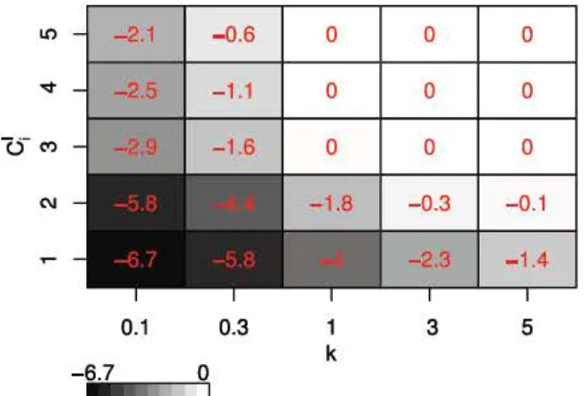
Policy Pl vs Policy P2.

Following Table 3, there are significant cor relations between Ll12 and the two parameters k and c1• Therefore, in

this paragraph, we first investigate how much more benefit Policy P2

provides over Policy Pl with different values of k and c1• The results are

sketched in Fig. 8.

Fig. 8 represents the relative decrease (Ll12

< 0)

between the op

timal costs of Policy P2 and Policy Pl. In other words, it characterizes the benefit provided by adjusted quality inspections when being in tegrated in the maintenance policy with fixed preventive replacement threshold. The shade of gray represents the value range of Ll12 : the

II) <SM N -2.1

-

0

.

6

0 -2.5 -1.1 0

-

-

-0.1 0.3

-

6.7

0

-1 k 0 0 0 0 0 0 -0.3 -0.1 -2.3 -1.4 3

5

Fig. 8. Performance of adjusted-quality inspections for fixed maintenance policy : Ll12 as a function of k (shape parameter of the inspection cost function) and c/ (cost of the low quality inspection) -With Cd

=

25, Cc

=

100, cP

=

50

darker, the greater the benefit of the adjusted quality inspection option

is. The horizontal axis represents the value of k the parameter char

acterizing the shape of the inspection cost function (see Eq. (15)) while the vertical axis characterizes the cost of low quality inspection (c/). Recall that if O

<

k

<

1, the inspection cost function is convex, whereas it is linear for k

=

1, and concave for k > 1.

When

k

increases, the benefit of adjusted quality inspections de creases. In other words,

if

the inspection cost decreases faster than the inspection quality, it is preferable to

use

adjusted quality inspections for fixed maintenance policy.

Consider for example the first column of Fig. 8, when k

=

0.1, using adjusted quality inspections helps to reduce from 2.1% to 6.7% of the

cost incurred by fixed inspection policy. However, when the inspection cost decreases slower than the inspection quality, (i.e. k

=

3 or 5), ad justed quality inspection cannot provide more benefit when compared with the non adjusted one (Ll12

=

0), especially for high inspection cost.

Indeed, the benefit of adjusted quality inspections decreases when the inspection cost increases. Since we consider a constant ratio between the high and low inspection cost, cNci = 3, if

c/

= 5, then

c

1h = 15, it is

preferable to

use

only inspections with low quality, which explains why the benefit of adjusted quality inspections decreases when k increases.

Proposed

Policy

P vs Policy P3.

Fig. 9 represents the relative decrease (Ll34

<

0) in the maintenance cost incurred by the Proposed Policy P

when compared to Policy P3. It characterizes the benefit provided by adjusted quality inspections when being integrated in a dynamic maintenance policy (with replacement option at every inspection period). The smaller the negative value of Ll34 is, the greater the benefit that the Proposed Policy P can provide when used instead of Policy P3.

The significations of color shades, horizontal and vertical axis are si milar to the ones of Fig. 8.

In the most favorable configurations (not too expensive inspections and convex inspection cost function), the Proposed Policy P allows

significant savings over Policy P3. The results show that when k in creases, the benefit provided by the Proposed Policy significantly de creases. This benefit also decreases with c;, showing that when the in spection cost is high, it is preferable to use low quality inspections. In

this latter case, the adjusted quality inspection policy tends to the fixed quality inspection policy.

4.4.3. Dynamic inspection vs dynamic mainlmance decision : performance

comparison

Policy P2 consists in the combination of dynamic inspections and a fixed maintenance decision rule whereas Policy P3 combines fixed in spections and a dynamic maintenance decision rule. Corresponding to every combination of the input parameters (c/, k, C,t,

vc,

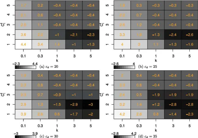
etc.) we find the minimum maintenance cost of the maintenance policies P2, P3 and then calculate the percentage of their difference, e.g. Ll2.3 given by Eq. (25).

II) _{0 0 0} "<t _{0 0 0} <S (') _{0 0} N 0 0 -0.3 0.1 0.3 1 3

5

k

-

5.4

0

Fig. 9. Performance of adjusted-quality inspections for dynamic replacement policy : ,¼. as a function of k (shape parameter of the inspection cost function) and c/ (cost of the low quality inspection) -With Cd

=

25, Cc

=

100, cP

=

50

It) It) _{0.3 -0.3 -0.3 -0.3}

v

v

-

-0.4 -0.4 -0.4

c:s

(') (')

-

-0.4 -0.4 -0.4 C\I C\I

-

-1.3 -2.4 -2.6 4.4 4 -1.3 -1.6 0.1 0.3 3 5 0.1 0.3 1 3 5 k It) It) _{0.4 -0.4 -0.4 -0.4}

v

v

-

-

-0.4 -0.4 -0.4

c:s

(') (')

-

0

.

5

-1 9 -1 9 -1.9 C\I C\I

-

-

-1.2 -2 8 -2.8

-

-

-

-1.4 -2.3 0.1 0.3 1 3 5 0.1 0.3 1 3 5 k k

-=

3

::

:

c:==

3:::J· 9 (c) Cd

=

30

-

=

2 ·:8

:

:

===

4

j'

2 (d} Cd

=

35

Fig. 10. Comparison of Policy P2 and Policy P3: d23 as a function of k (shape parameter of the inspection cost function) and

c/

(cost of the low quality inspection)

-Cc

=

100, Cp

=

50 -For different values of c.i

Based on the evolution of Ll₂₃ as a function of different system para

meters, the aim of this section is to compare more in depth the behavior

and the performance of these two policies P2 and P3 to gain a better

understanding of their respective interests.

Fig. 10 presents the performance difference between Policy P3 and

Policy P2 : Policy P2 is better than Policy P3 when Ll23 > 0 and in

versely. The values of Ll2_3 are then illustrated by shades of black: the

darker, the smaller value of Ll2.3 is. It can be observed that

• !l23 is positive for all cases of k between k

=

0.1 and 0.3, which in

dicates that the performance of the adjusted quality policy is better

than the one of the dynamic replacement policy when the inspection

cost decreases faster than the inspection quality (k

<

1).

• When k

=

1, it is preferable to

use

Policy 2 with adjusted quality

inspections to reduce the maintenance cost for low inspection cost

(

c/

=

1). When the inspection cost increases, the performance of

adjusted quality inspection decreases, then the performance of

Policy P3 is better than the one of Policy P2.

• When k

=

3 or 5, the inspection cost increases faster than the in

spection quality, and it is not possible to take advantage from an

adjusted quality inspection policy. In this case, it preferable to

use

Policy P3 with a dynamic replacement option to reduce the main tenance cost.

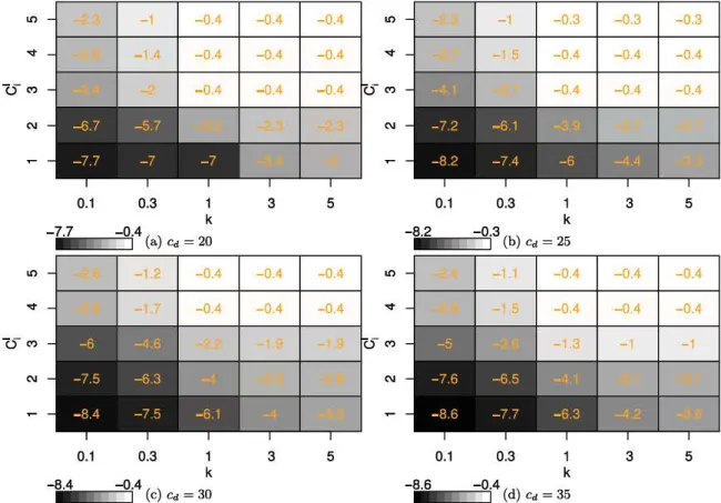
On the other hand, Fig. 11 presents the evolution of Ll23 with the

variance coefficient of the deterioration process vc and the shape

coefficient of the inspection cost function k.

It can be seen in Fig. 11 that Ll₂_3 is not monotone when

vc

increases,

which explains why the correlation value of Ll23 and vc is low, see

Table 3. However, an interesting result can be recognized: when

vc

increases from 0.1 to 0.3 or 0.5, Ll23 increases as well It is thus pre

ferable to use Policy P2 with adjusted quality inspections than Policy

P3 with fixed quality inspections when the variance coefficient

vc

of the

I'-0

It)

0

0 > (')

0

~

0

•

•

0.7 0.2

••

•

2

••

4

•

•

0.1 -1.6

Mi

3 0.3 5.2 1.1

1

k -1.3 3 0.2 1.3 -0.1 -1.6 5

Fig. 11. Comparison of Policy P2 and Policy P3 for different values of the

variance coefficient vc and the shape parameter of the cost function k -With

Cd

=

25,

c,

=

100, Cp

=

50 and

c/

=

1

degradation process increases. However, ifvc is very high, e.g. vc

=

0.7,

the high quality inspections might not be necessary. Therefore, the

performance of adjusting quality inspections decreases and then, the

value of !l23 also decreases when

vc

increases from 0.5 to 0.7.

4.4.4.

Performance of dynamic inspection mainlmance policy

In this section, we investigate the performance gain brought by the

dynamic inspection maintenance policy (P) over the classic CBM. In

detail, corresponding to every combination of the input parameters (ea,

k,

cf

,

etc.) we find the optimal values of the policies P and Pl and then

calculate the percentage of their difference, e.g. Ll14 given by Eq. (25).

The performance gain brought by the policy P over the policy Pl is

represented in Fig. 12. We find that in all cases, Ll14 is negative, the