HAL Id: pastel-00679369
https://pastel.archives-ouvertes.fr/pastel-00679369
Submitted on 15 Mar 2012HAL is a multi-disciplinary open access archive for the deposit and dissemination of sci-entific research documents, whether they are pub-lished or not. The documents may come from teaching and research institutions in France or abroad, or from public or private research centers.
L’archive ouverte pluridisciplinaire HAL, est destinée au dépôt et à la diffusion de documents scientifiques de niveau recherche, publiés ou non, émanant des établissements d’enseignement et de recherche français ou étrangers, des laboratoires publics ou privés.
measurements: measurements and modelling
Caleb Narasigadu
To cite this version:
Caleb Narasigadu. Design of a static micro-cell for phase equilibrium measurements: measurements and modelling. Chemical and Process Engineering. École Nationale Supérieure des Mines de Paris; University of KwaZulu-Natal - Afrique du Sud, 2011. English. �NNT : 2011ENMP0071�. �pastel-00679369�
MINES ParisTech
Centre Énergétique et Procédés – Laboratoire CEP/TEP 35, rue Saint Honoré, 77305 Fontainebleau cedex, France
i
École doctorale n° 432 : Sciences des Métiers de l’lngénieur
présentée et soutenue publiquement par
Caleb NARASIGADU
le 06 septembre 2011Conception ďune Micro-Cellule pour Mesures d’Équilibres de Phases :
Mesures et Modélisation
Design of a Static Micro-Cell for Phase Equilibrium Measurements :
Measurements and Modelling
Doctorat ParisTech
T H È S E
pour obtenir le grade de docteur délivré par
l’École nationale supérieure des mines de Paris
Spécialité « Génie des Procédés »
Directeurs de thèse : Dominique RICHON et Deresh RAMJUGERNATH Co-encadrements de la thèse : Christophe COQUELET et Paramespri NAIDOO
T
H
È
S
E
JuryM. Jean-Nöel JAUBERT, Professeur, Institut National Polytechnique de Lorraine Rapporteur M. Serge LAUGIER, Maitre de Conférence, E.N.S.C.B.P. Rapporteur M. Johan David RAAL, Professeur Emerite, University of KwaZulu-Natal Examinateur M. Pascal MOUGIN, Ingénieur de Recherche, Institut français du pétrole Examinateur M. Deresh RAMJUGERNATH, Professeur, University of KwaZulu-Natal Examinateur M. Dominique RICHON, Directeur de Recherche, MINES ParisTech Examinateur M. Christophe COQUELET, Maitre Assistant, MINES ParisTech Examinateur
ii
DESIGN OF A STATIC MICRO-CELL FOR PHASE
EQUILIBRIUM MEASUREMENTS:
MEASUREMENTS AND MODELLING
by
CALEB NARASIGADU
[MSc. (Eng)]
University of KwaZulu Natal
Submitted in fulfillment of the academic requirements for
the degree of Doctor of Philosophy in Engineering at the School
of Chemical Engineering, University of KwaZulu Natal and
L’Ecole Nationale Supérieure des Mines de Paris
as agreed in the convention for international joint doctorate supervision
entered into by these two institutions
Durban
2011
iii
ABSTRACT
Vapour-Liquid Equilibrium (VLE), Liquid-Liquid Equilibrium (LLE) and Vapour-Liquid-Liquid Equilibrium (VLLE) are of special interest in chemical engineering as these types of data form the basis for the design and optimization of separation processes such as distillation and extraction, which involve phase contacting. Of recent, chemical companies/industries have required thermodynamic data (especially phase equilibrium data) for chemicals that are expensive or costly to synthesize. Phase equilibrium data for such chemicals are scarce in the open literature since most apparatus used for phase equilibrium measurements require large volumes (on average 120 ) of chemicals. Therefore, new techniques and equipment have to be developed to measure phase equilibrium for small volumes across reasonable temperature and pressure ranges.
This study covers the design of a new apparatus that enables reliable vapour pressure and equilibria measurements for multiple liquid and vapour phases of small volumes (a maximum of 18 ). These phase equilibria measurements include: VLE, LLE and VLLE. The operating temperature of the apparatus ranges from 253 to 473 K and the operating pressure ranges from absolute vacuum to 1600 kPa. The sampling of the phases are accomplished using a single Rapid-OnLine-Sampler-Injector () that is capable of withdrawing as little as 1μl of sample from each phase. This ensures that the equilibrium condition is not disturbed during the sampling and analysis process. As an added advantage, a short equilibrium time is generally associated with a small volume apparatus. This enables rapid measurement of multiple phase equilibria. A novel technique is used to achieve sampling for each phase. The technique made use of a metallic rod (similar in dimension to the capillary of the ) in an arrangement to compensate for volume changes during sampling.
As part of this study, vapour pressure and phase equilibrium data were measured to test the operation of the newly developed apparatus that include the following systems:
• VLE for 2-methoxy-2-methylpropane + ethyl acetate at 373.17 K • LLE for methanol + heptane at 350 kPa
• LLE for hexane + acetonitrile at 350 kPa • VLLE for hexane + acetonitrile at 348.20 K
New experimental vapour pressure and VLE data were also measured for systems of interest to petrochemical companies. These measurements include:
iv
• VLE for ethanol + butan-2-one at 383.26, 398.23 and 413.21 K • VLE for ethanol + 2-methoxy-2-methylbutane at 398.25 and 413.19 K • VLE for ethanol + 2-methylpent-2-ene at 383.20 K
These measurements were undertaken to understand the thermodynamic interactions of light alcohols and carbonyls as part of a number of distillation systems in synthetic fuel refining processes which are currently not well described. Two of these above mentioned systems include expensive chemicals: 2-methoxy-2-methylbutane and 2-methylpent-2-ene.
The experimental vapour pressure data obtained were regressed using the extended Antoine and Wagner equations. The experimental VLE data measured were regressed with thermodynamic models using the direct and combined methods. For the direct method the Soave-Redlich-Kwong and Peng-Robinson equations of state were used with the temperature dependent function (α) of Mathias and Copeman (1983). For the combined method, the Virial equation of state with the second Virial coefficient correlation of Tsonopoulos (1974) was used together with one of the following liquid-phase activity coefficient model: TK-Wilson, NRTL and modified UNIQUAC. Thermodynamic consistency testing was also performed for all the VLE experimental data measured where almost all the systems measured showed good thermodynamic consistency for the point test of Van Ness et al. (1973) and direct test of Van Ness (1995).
v
PREFACE
The work presented in this thesis was performed at the University of KwaZulu-Natal and L’Ecole Nationale Supérieure des Mines de Paris from January 2008 to March 2011 as stipulated in the convention for international joint doctorate supervision entered into by these two institutions. The work was supervised by Professor D. Ramjugernath and Doctor P. Naidoo at the University of KwaZulu-Natal and Prof. D. Richon and Doctor C. Coquelet at L’Ecole Nationale Supérieure des Mines de Paris.
This thesis is submitted as the full requirement for the degree PhD in chemical engineering.
I, Caleb Narasigadu declare that:
i) The research in this dissertation, except where otherwise stated, is my original work. ii) This thesis has not been submitted for any degree or examination at any other university. iii) This thesis does not contain other persons’ data, pictures, graphs or other information,
unless specifically acknowledged as being sourced from other persons.
iv) This thesis does not contain other persons’ writing, unless specifically acknowledged as being sourced from other researchers. Where other written sources have been quoted then:
a)
Their words have been re-written but the general information attributed to them has been referenced;b)
Where their exact words have been used, their writing has been placed inside quotation marks and referenced.v) This thesis does not contain text, graphics or tables copied and pasted from the internet, unless specifically acknowledged and the source being detailed in the thesis and in the References section.
__________________ C. Narasigadu
As supervisor of this candidate, I approve this dissertation for submission:
______________________ _____________________
Professor D. Ramjugernath Doctor P. Naidoo
______________________ _____________________
vi
ACKNOWLEDGEMENTS
I would like to take this opportunity to acknowledge and thank the following who have made a tremendous contribution to this work:
• Firstly, my Lord and Saviour, Jesus Christ, Who has made my tertiary education a reality. Lord, I am eternally grateful to You.
• My supervisors, Professor D. Ramjugernath, Doctor P. Naidoo, Doctor C. Coquelet and Professor D. Richon for their expert knowledge, guidance and support.
• SASOL Ltd. for their financial assistance.
• The technical staff at the School of Chemical Engineering University of KwaZulu Natal, in particular Kelly Robertson for his invaluable contribution to this work in terms of construction work.
• Alan Raymond Foster and Warren Errol Sheahan for their assistance with the schematic drawings.
• My mum, Linda, my sister, Lisa, and my uncle and aunt, Jiva and Sylvia, for their many years of wholehearted support, prayer, encouragement, love and motivation.
• My extended family, fellow postgraduate colleagues, friends and especially the congregation of Christian Revival Centre Tongaat church for their invaluable advice, prayer, support and friendship.
vii
DEDICATION
To
my Lord and Saviour, Jesus Christ
But without faith it is impossible to please and be satisfactory to Him. For whoever would come near to God must [necessarily] believe
that God exists and that He is the rewarder of those who earnestly and diligently seek Him [out].
HEBREWS 11:6
viii
TABLE OF CONTENTS
ABSTRACT
………...
iii
PREFACE
………..………...
v
ACKNOWLEDGEMENTS
………..…….
vi
TABLE OF CONTENTS
………...
viii
LIST OF FIGURES
………..………..
xiv
LIST OF PHOTOGRAPHS
………...
xxvi
LIST OF TABLES
………...
xxvii
NOMENCLATURE
………...
xxxi
CHAPTER 1:
FRENCH SUMMARY
...
1
INTRODUCTION
………...
2
CHAPTER 2:
FRENCH SUMMARY
………...…
4
LITERATURE REVIEW
...
6
2.1 The Static Method……….
7
2.2 Cell Design……….……….
8
2.2.1 Material of Construction……….
9
2.2.2 Thermal Environment………..………...
9
2.2.3 Agitation of Cell Contents……….
11
2.3 Sampling Techniques………..…
15
ix
CHAPTER 3:
FRENCH SUMMARY
………...….
22
THERMODYNAMIC FUNDAMENTALS AND
PRINCIPLES
……….
24
3.1 Fugacity and Fugacity Coefficients………..
25
3.1.1 Fugacity Coefficients from the Virial Equation of State……..…..
30
3.1.2 Fugacity Coefficients from a Cubic Equation of State…………...
33
3.1.2.1 The Soave-Redlich-Kwong (SRK) Cubic Equation of State
…...
33
3.1.2.2 The Peng-Robinson (PR) Cubic Equation of State
…..………..
36
3.1.2.3 The Alpha Correlation of Mathias and Copeman. (1983)……...
37
3.1.3 Mixing Rules for Cubic Equations of State……….
38
3.2 Activity and Activity Coefficient………..….
40
3.2.1 Liquid Phase Activity Coefficient Models………....
43
3.2.1.1 The Tsuboka-Katayama-Wilson (TK-Wilson) Equation
……...
43
3.2.1.2 The NRTL (Non-Random Two Liquid) Equation
………..
45
3.2.1.3The Modified UNIQUAC (UNIversal QUasi-Chemical) Equation
……….
47
3.3 Vapour-Liquid Equilibrium (VLE)………..……
49
3.3.1 VLE Data Regression………..………...
50
3.3.1.1 The Combined (γ-Ф) Method
……….…..
52
3.3.1.2 The Direct (Ф-Ф) Method
………....
55
3.4 Liquid-Liquid Equilibrium (LLE)………..…..
59
3.4.1 Binary Systems………...
59
3.4.2 Theoretical Treatment of LLE………..…
60
3.4.3 Binary LLE Data Regression………....
62
3.5 Vapour-Liquid-Liquid Equilibrium (VLLE)………..…
363
3.5.1 VLLE Data Regression………..………
66
3.6 Thermodynamic Consistency Tests………..………
66
3.6.1 The Point Test……….
67
3.6.2 The Direct Test………...
68
x
EQUIPMENT DESCRIPTION
………...
73
4.1 Description of the Equilibrium Cell and its Housing……….
74
4.2 Sampling Technique and Assembly………..
77
4.3 Method of Agitation within the Equilibrium Cell……….78
4.4 Isothermal Environment for the Equilibrium Cell………...
80
4.5 Temperature and Pressure Measurement……….
82
4.5.1 Temperature Measurement………...
82
4.5.2 Pressure Measurement………..
82
4.6 Composition Analysis………..
83
4.7 Data Logging………
86
4.8 Degassing Apparatus………...
86
4.9 Compression Device for Cell Loading………...
88
4.10 Safety Features………...
89
4.11 Overview……….
91
CHAPTER 5:
FRENCH SUMMARY
………....
92
EXPERIMENTAL PROCEDURE
……….
94
5.1 Degassing Apparatus………..…………....
95
5.1.1 Preparation……….
95
5.1.2 Cleaning of the Degassing Apparatus………..….95
5.1.3 Operating Procedure of the Degassing Apparatus……….
96
5.2 Compression Device………..………..
98
5.2.1 Preparation and Cleaning………...
98
5.2.2 Charging the Compression Device….………..
98
5.3 Phase Equilibrium Apparatus………..
100
5.3.1 Preparation………...…
100
5.3.1.1 Leak Detection……….. 100
5.3.1.2 Cleaning the Equilibrium Cell………. 101
5.3.2 Calibration………
103
5.3.2.1 Temperature Probe Calibration………... 103
xi
5.3.2.3 Gas Chromatograph Calibration………. 104
5.3.3 Operating Procedures for Phase Equilibrium Measurements….
106
5.3.3.1 In-Situ Degassing………. 1065.3.3.2 Vapour Pressure Measurement………... 107
5.3.3.3 Binary Vapour-Liquid Equilibrium (VLE) Measurement……. 109
5.3.3.4 Binary Liquid-Liquid Equilibrium (LLE) Measurement……... 113
5.3.3.5 Binary Vapour-Liquid-Liquid Equilibrium (VLLE) Measurement. .……….. 115
CHAPTER 6:
FRENCH SUMMARY
………...…
117
EXPERIMENTAL RESULTS
………...
119
6.1 Chemical Purity……….120
6.2 Experimental Uncertainties……….
120
6.3 Vapour Pressure Data……….……….
122
6.4 Phase Equilibria of Test Systems………...
127
6.4.1 Vapour-Liquid Equilibrium (VLE) Result………
127
6.4.1.1 2-Methoxy-2-Methylpropane (1) + Ethyl Acetate (2)
……...
1276.4.2 Liquid-Liquid Equilibrium (LLE) Results………
129
6.4.2.1 Hexane (1) + Acetonitrile (2)
………..
1296.4.2.2 Methanol (1) + Heptane (2)
………
1306.5 Phase Equilibria of New Systems……….
131
6.5.1 Vapour-Liquid Equilibrium (VLE)………
131
6.5.1.1 Methanol (1) + Butan-2-one (2)……….. 131
6.5.1.2 Ethanol (1) + Butan-2-one (2)………. 133
6.5.1.3 Ethanol (1) + 2-Methoxy-2-Methylbutane (2)………. 135
6.5.1.4 2-Methylpent-2-ene (1) + Ethanol (2)………..137
6.5.2 Vapour-Liquid-Liquid Equilibrium (VLLE)………
139
6.5.2.1 Hexane (1) + Acetonitrile (2)………... 139
CHAPTER 7:
FRENCH SUMMARY
………..……
142
DATA ANALYSIS AND DISCUSSION
……….
143
xii
7.2 Experimental Vapour Pressure Data………...
144
7.2.1 Comparison of Experimental and Literature Vapour Pressure..
145
7.2.2 Regression using Empirical Correlations……….….
149
7.2.3 Regression using Equations of State………...
150
7.2.4 Thermodynamic Consistency Testing for Vapour Pressure Data….
……….
156
7.3 Experimental Activity Coefficients – VLE/VLLE Systems……….…...
156
7.4 Experimental VLE Data Reduction………160
7.4.1 2-Methoxy-2-Methylpropane (1) + Ethyl Acetate (2)…………...
161
7.4.2 Methanol (1) + Butan-2-one (2)…………..……….
167
7.4.3 Ethanol (1) + Butan-2-one (2)………..
172
7.4.4 Ethanol (1) + 2-Methoxy-2-Methylbutane (2)………
177
7.4.5 2-Methylpent-2-ene (1) + Ethanol (2)……….
182
7.5 Experimental LLE Data Reduction……….…...
188
7.5.1 Hexane (1) + Acetonitrile (2)……….…………..
188
7.5.2 Methanol (1) + Heptane (2)……….………
191
7.6 Experimental VLLE Data Reduction………
194
7.6.1 Hexane (1) + Acetonitrile (2)………...
194
7.7 Thermodynamic Consistency Testing for VLE Systems……….
198
7.7.1 2-Methoxy-2-Methylpropane (1) + Ethyl Acetate (2)…………...
199
7.7.2 Methanol (1) + Butan-2-one (2)………...
202
7.7.3 Ethanol (1) + Butan-2-one (2)………..
206
7.7.4 Ethanol (1) + 2-Methoxy-2-Methylbutane (2)………
210
7.7.5 2-Methylpent-2-ene (1) + Ethanol (1)……….
213
7.8 Concluding Remarks……….
216
CHAPTER 8:
FRENCH SUMMARY
………...…
217
CONCLUSION
………...
219
CHAPTER 9:
FRENCH SUMMARY
………...….
222
xiii
REFERENCES
………..………..
225
APPENDIX A: CRITERION FOR PHASE EQUILIBRIUM
……..…
242
APPENDIX B: PHYSICAL PROPERTIES OF CHEMICALS
...
245
APPENDIX C: CALIBRATIONS
………..………...
246
C.1 Temperature Calibrations……….………..246
C.2 Pressure Calibrations………...…
259
C.3 Gas Chromatograph Conditions……….
261
C.4 Gas Chromatograph Calibrations………...
263
C.4.1 VLE Systems………
263
C.4.2 LLE and VLLE Systems……….
272
APPENDIX D: USER-INTERFACE OF SOFTWARE
……….……...
276
APPENDIX E: APPARATUS FLOW DIAGRAM
………
278
APPENDIX F: COMMUNICATIONS
………..………
279
F.1 Publications……….…….………..279
F.2 Conferences……….……...…
279
xiv
LIST OF FIGURES
Chapter 2
Figure 2-1: Schematic illustration of the static analytical method (Raal and Mühlbauer, 1998)………...8 Figure 2-2: Schematic of the experimental apparatus of Outcalt and Lee (2004)……….. 10 Figure 2-3: Equilibrium cell and agitator of Bae et al. (1981)……… 12 Figure 2-4: Schematic illustration of the equilibrium cell and auxillary equipment of Huang et al. (1985)………...13
Figure 2-5: Equilibrium cell of Ashcroft et al. (1983)………14
Figure 2-6: Schematic of the acoustic interferometer used for bubble point pressure measurements by Takagi et al. (2003)………..14 Figure 2-7: (a) Equilibrium cell assembly of Figuiere et al. (1980); (b) carrier gas circulation through the cell to sweep samples (cross section 1-1)……….16
Figure 2-8: Equilibrium cell of Legret et al. (1981)………17
Figure 2-9: Sampling microcell of Legret et al. (1981)………..17
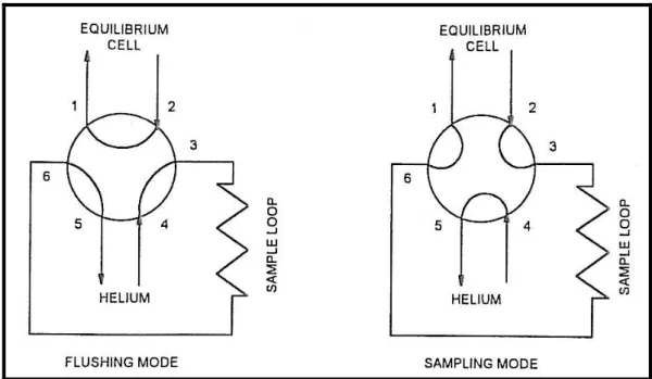
Figure 2-10: Equilibrium cell and sampling system of Rogers and Prausnitz (1970)…………..18 Figure 2-11: Sampling configuration of the six-port gas chromatograph valve used by
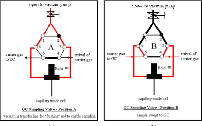
Ramjugernath (2000) (Raal and Mühlbauer, 1998)……….19 Figure 2-12: Electromagnetic version of sampler ( Evolution IV)…………19
Figure 2-13: Schematic of the degassing apparatus of Van Ness and Abbott (1978)…………...21 Figure 2-14: Purification and degassing apparatus of Fischer and Gmehling (1994)…………...21
Chapter 3
Figure 3-1: The three common types of binary phase diagrams for T-x-y, P-x-y and x-y plots: (a) intermediate-boiling; (b) minimum boiling azeotrope; (c) maximum boiling azeotrope (Raal and Mühlbauer, 1998)………..………..50 Figure 3-2: Calculation flow diagram for the bubble point pressure procedure of the combined
method to obtain the parameters for the liquid phase activity coefficient model (Smith et al., 2001)………...54 Figure 3-3: Calculation flow diagram for the bubble point pressure iteration for the direct
xv
Figure 3-4: Three types of constant pressure binary LLE phase diagrams: (a) an island curve, (b) a convex curve and (c) a concave curve, where α and β refer to the two liquid phases (Smith et al., 2001)………...60 Figure 3-5: Molar Gibbs energy of mixing for a partially miscible binary system at constant
temperature and pressure (Prausnitz et al., 1999)……….61 Figure 3-6: A common T-x-y diagram at constant pressure for a binary system exhibiting VLLE (Smith et al., 2001)………...64 Figure 3-7: A common P-x-y diagram at constant temperature for a binary system exhibiting
VLLE (Smith et al., 2001)………65
Chapter 4
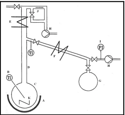
Figure 4-1: Schematic of the equilibrium cell assembly……….79
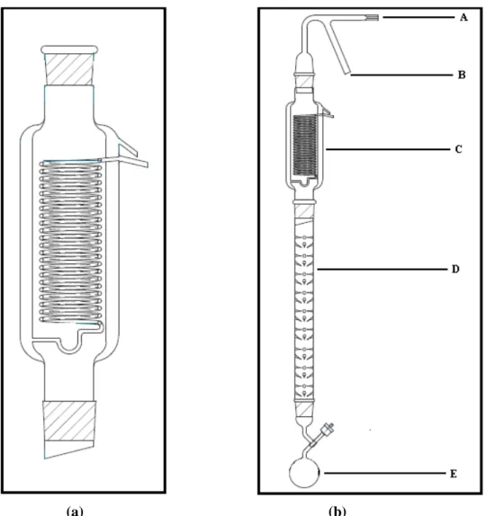
Figure 4-2: Positions of the GC sampling valve during operation for (a) “flushing” and (b) sampling………...85 Figure 4-3: Schematic of the (a) total condenser and (b) the degassing unit assembly………..87
Figure 4-4: Schematic of the compression device………...89
Chapter 5
Figure 5-1: Schematic of the set-up for charging the compression device………...… 100 Figure 5-2: Schematic of the set-up for charging the equilibrium cell with degassed liquid from
the boiling flask………..… 108
Figure 5-3: Schematic of the set-up for charging the second component into the equilibrium cell………..110
Chapter 6
Figure 6-1: Vapour pressure plots for the ethers used in this study, 2-methoxy-2-methylbutane and 2-methoxy-2-methylpropane, compared to literature. Error bars show 1 % error for pressure and 0.5 % error for temperature……….124
xvi
Figure 6-2: Vapour pressure plots for the alcohols used in this study, ethanol and methanol, compared to literature. Error bars show 1 % error for pressure and 0.5 % error for temperature……….125 Figure 6-3: Vapour pressure plots for the ketone (butan-2-one) and ester (ethyl acetate) used in
this study compared to literature. Error bars show 1 % error for pressure and 0.5 % error for temperature………...125 Figure 6-4: Vapour pressure plots for the alkanes used in this study, heptane and hexane,
compared to literature. Error bars show 1 % error for pressure and 0.5 % error for temperature……….126 Figure 6-5: Vapour pressure plots for the alkene (2-methylpent-2-ene) and nitrile (acetonitrile)
used in this study compared to literature. Error bars show 1 % error for pressure and 0.5 % error for temperature……….126 Figure 6-6: The x-y plot for the 2-methoxy-2-methylpropane (1) + ethyl acetate (2) system at
373.17 K, error bars show 2% error for and ………..128 Figure 6-7: The P-x- y plot for the 2-methoxy-2-methylpropane (1) + ethyl acetate (2) system at
373.17 K, error bars show 1% error for pressure and 2% error for and ……128 Figure 6-8: The T-- plot for the hexane (1) + acetonitrile (2) system at 350 kPa, error bars show
0.3% error for temperature and 2% error for and ………..129
Figure 6-9: The T-- plot for the methanol (1) + heptane (2) system at 350 kPa, error bars show 0.3% error for temperature and 2% error for and ………..130
Figure 6-10: The x-y plot for the methanol (1) + butan-2-one (2) system, error bars show 2% error for and ………...………132 Figure 6-11: The P-x-y plot for the methanol (1) + butan-2-one (2) system, error bars show 1%
error for pressure and 2% error for and ……….133 Figure 6-12: The x-y plot for the ethanol (1) + butan-2-one (2) system, error bars show 2% error
for and ………134 Figure 6-13: The P-x-y plot for the ethanol (1) + butan-2-one (2) system, error bars show 1%
error for pressure and 2% error for and ……….135 Figure 6-14: The x-y plot for the ethanol (1) + 2-methoxy-2-methylbutane (2) system, error bars
show 2% error for and ………136 Figure 6-15: The P-x-y plot for the ethanol (1) + 2-methoxy-2-methylbutane (2) system, error
bars show 1% error for pressure and 2% error for and ………..137 Figure 6-16: The x-y plot for the 2-methylpent-2-ene (1) + ethanol (2) system at 383.20 K, error
xvii
Figure 6-17: The P-x-y plot for the 2-methylpent-2-ene (1) + ethanol (2) system at 383.20 K, error bars show 1% error for pressure and 2% error for and ……….139 Figure 6-18: The - -y plot for the hexane (1) + acetonitrile (2) system at 348.20 K, error bars
show 2% error for , and ………140 Figure 6-19: The P-- -y plot for the hexane (1) + acetonitrile (2) system at 348.20 K, error bars
show 1% error for pressure and 2% error for , and ………..141
Chapter 7
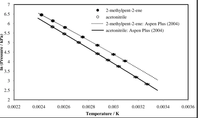
Figure 7-1: Vapour pressure deviation plots for the comparison of experimental data with Aspen Plus (2004) for 2-methoxy-2-methylbutane and experimental data with Reid et al. (1988) for 2-methoxy-2-methylpropane………145 Figure 7-2: Vapour pressure deviation plots for the comparison of experimental data with Reid
et al. (1988) for ethanol and experimental data with Aspen Plus (2004) for methanol………...………..146 Figure 7-3: Vapour pressure deviation plots for the comparison of experimental data with Reid
et al. (1988) for butan-2-one and experimental data with Aspen Plus (2004) for ethyl acetate……….………...146 Figure 7-4: Vapour pressure deviation plots for the comparison of experimental data with Reid
et al. (1988) for heptane and hexane………..147 Figure 7-5: Vapour pressure deviation plots for the comparison of experimental data with
Aspen Plus (2004) for 2-methylpent-2-ene and experimental data with Reid et al. (1988) for acetonitrile………...147 Figure 7-6: Vapour pressure plots for the ethers used in this study, 2-methoxy-2-methylbutane and 2-methoxy-2-methylpropane, with the best fit of the empirical correlations. Error bars show 1 % error for pressure and 0.5 % error for temperature………...152 Figure 7-7: Vapour pressure plots for the alcohols used in this study, ethanol and methanol,
with the best fit of the empirical correlations. Error bars show 1 % error for pressure and 0.5 % error for temperature………...154 Figure 7-8: Vapour pressure plots for the ketone (butan-2-one) and ester (ethyl acetate) used in
this study with the best fit of the empirical correlations. Error bars show 1 % error for pressure and 0.5 % error for temperature……….154
xviii
Figure 7-9: Vapour pressure plots for the alkanes used in this study, heptane and hexane, with the best fit of the empirical correlations. Error bars show 1 % error for pressure and 0.5 % error for temperature………155 Figure 7-10: Vapour pressure plots for the alkene (2-methylpent-2-ene) and nitrile (acetonitrile)
used in this study with the best fit of the empirical correlations. Error bars show 1 % error for pressure and 0.5 % error for temperature………155 Figure 7-11: Fit of the TS-NRTL model combination to the x-y plot of the methoxy-2-methylpropane (1) + ethyl acetate (2) system at 373.17 K for the combined method………164 Figure 7-12: Fit of the TS-NRTL model combination to the P-x-y plot of the methoxy-2-methylpropane (1) + ethyl acetate (2) system at 373.17 K for the combined method………164 Figure 7-13: Comparison of the experimental activity coefficients and those calculated from the
TS-NRTL model combination for the 2-methoxy-2-methylpropane (1) + ethyl acetate (2) system at 373.17 K for the combined method………..165 Figure 7-14: Fit of the PR-MC-WS-NRTL model combination to the x-y plot of the 2-methoxy-2-methylpropane (1) + ethyl acetate (2) system at 373.17 K for the direct method………166 Figure 7-15: Fit of the PR-MC-WS-NRTL model combination to the P-x-y plot of the 2-methoxy-2-methylpropane (1) + ethyl acetate (2) system at 373.17 K for the direct method………166 Figure 7-16: Best fit model combination for the x-y plot of the methanol (1) + butan-2-one (2)
system with the combined method……….169 Figure 7-17: Best fit model combination (383.25 K: TS-TKWILSON; 398.14 K: TS-NRTL;
413.20 K: TS-TKWILSON) to the P-x-y plot of the methanol (1) + butan-2-one (2) system with the combined method……….170 Figure 7-18: Comparison of the experimental activity coefficients and those calculated from the
best fit model combination for the methanol (1) + butan-2-one (2) system with the combined method………...170 Figure 7-19: Best fit model combination for the x-y plot of the methanol (1) + butan-2-one (2)
system with the direct method………171 Figure 7-20: Best fit model combination (383.25 K: PR-MC-WS-NRTL; 398.14 K:
SRK-MC-WS-NRTL; 413.20 K: PR-MC-WS-NRTL) to the P-x-y plot of the methanol (1) + butan-2-one (2) system with the direct method………..172
xix
Figure 7-21: Best fit model combination for the x-y plot of the ethanol (1) + butan-2-one (2) system with the combined method……….174 Figure 7-22: Best fit model combination (383.26 K: TS-UNIQUAC; 398.23 K: TS-UNIQUAC;
413.20 K: TS-NRTL) to the P-x-y plot of the ethanol (1) + butan-2-one (2) system with the combined method……….175 Figure 7-23: Comparison of the experimental activity coefficients and those calculated from the
best fit model combination for the ethanol (1) + butan-2-one (2) system with the combined method………...175 Figure 7-24: Best fit model combination for the x-y plot of the ethanol (1) + butan-2-one (2)
system with the direct method………176 Figure 7-25: Best fit model combination (383.26, 398.23 and 413.21 K: SRK-MC-WS-NRTL) to the P-x-y plot of the ethanol (1) + butan-2-one (2) system with the direct method………177 Figure 7-26: Best fit model combination for the x-y plot of the ethanol (1) + 2-methoxy-2-methylbutane (2) system with the combined method……….179 Figure 7-27: Best fit model combination (398.25 and 413.19 K: TS-NRTL) to the P-x-y plot of the ethanol (1) + 2-methoxy-2-methylbutane (2) system with the combined method………180 Figure 7-28: Comparison of the experimental activity coefficients and those calculated from the
best fit model combination for the ethanol (1) + 2-methoxy-2-methylbutane (2) system with the combined method……….180 Figure 7-29: Best fit model combination for the x-y plot of the ethanol (1) + 2-methoxy-2-methylbutane (2) system with the direct method………...181 Figure 7-30: Best fit model combination (398.23 K: PR-MC-WS-NRTL and 413.21 K: SRK-MC-WS-NRTL) to the P-x-y plot of the ethanol (1) + 2-methoxy-2-methylbutane (2) system with the direct method………..182 Figure 7-31: Fit of the TS-NRTL model combination to the x-y plot of the 2-methylpent-2-ene
(1) + ethanol (2) system at 383.20 K for the combined method……….184 Figure 7-32: Fit of the TS-NRTL model combination to the P-x-y plot of the 2-methylpent-2-ene (1) + ethanol (2) system at 383.20 K for the combined method……….184 Figure 7-33: Comparison of the experimental activity coefficients and those calculated from the TS-NRTL model combination for the 2-methylpent-2-ene (1) + ethanol (2) system at 383.20 K for the combined method………185
xx
Figure 7-34: Comparison of the vapour pressures of ethanol and 2-methylpent-2-ene showing the Bancroft point………185 Figure 7-35: Fit of the PR-MC-WS-NRTL model combination to the x-y plot of the
2-methylpent-2-ene (1) + ethanol (2) system at 383.20 K for the direct method…..187 Figure 7-36: Fit of the PR-MC-WS-NRTL model combination to the P-x-y plot of the 2-methylpent-2-ene (1) + ethanol (2) system at 383.20 K for the direct method…..187 Figure 7-37: Temperature dependence of the TK-Wilson model parameters for the hexane (1) +
acetonitrile (2) system………189 Figure 7-38: Temperature dependence of the NRTL model parameters for the hexane (1) +
acetonitrile (2) system………190 Figure 7-39: Temperature dependence of the modified UNIQUAC model parameters for the
hexane (1) + acetonitrile (2) system………...190 Figure 7-40: Temperature dependence of the TK-Wilson model parameters for the methanol (1)
+ heptane (2) system………...192 Figure 7-41: Temperature dependence of the NRTL model parameters for the methanol (1) +
heptane (2) system………..193 Figure 7-42: Temperature dependence of the modified UNIQUAC parameters for the methanol
(1) + heptane (2) system……….193 Figure 7-43: Fit of the TS-TKWILSON model combination to the x-y plot of the hexane (1) +
acetonitrile (2) system at 348.20 K for the combined method………...196 Figure 7-44: Fit of the TS-TKWILSON model combination to the P-x-y plot of the hexane (1) +
acetonitrile (2) system at 348.20 K for the combined method………...196 Figure 7-45: Comparison of the P-x-y prediction plot using the parameters regressed from LLE
and VLLE data with the TK-Wilson model for the hexane (1) + acetonitrile (2) system at 348.20 K……….197 Figure 7-46: Comparison of the molar Gibbs energy of mixing using the parameters regressed
from LLE and VLLE data with the TK-Wilson model for the hexane (1) + acetonitrile (2) system at 348.20 K……….197 Figure 7-47: ∆P plot for the TS-NRTL and PR-MC-WS-NRTL model combinations for the
2-methoxy-2-methylpropane (1) + ethyl acetate (2) system at 373.17 K…………200 Figure 7-48: ∆ plot for the TS-NRTL and PR-MC-WS-NRTL model combinations for the
2-methoxy-2-methylpropane (1) + ethyl acetate (2) system at 373.17 K…………..201 Figure 7-49: ∆ ln (γ/γ) plot for the TS-NRTL model combination for the
xxi
Figure 7-50: ∆P plot for the best fit direct method model combinations of the methanol (1) + butan-2-one (2) system at 383.25, 398.14 and 413.20 K………...202 Figure 7-51: ∆ plot for the best fit direct method model combinations of the methanol (1) +
butan-2-one (2) system at 383.25, 398.14 and 413.20 K………...203 Figure 7-52: ∆P plot for the best fit combined method model combinations of the methanol (1) +
butan-2-one (2) system at 383.25, 398.14 and 413.20 K………...204 Figure 7-53: ∆ plot for the best fit combined method model combinations of the methanol (1) +
butan-2-one (2) system at 383.25, 398.14 and 413.20 K………204 Figure 7-54: ∆ ln (γ/γ) plot for the combined method best fit model combinations of the methanol
(1) + butan-2-one (2) system at 383.25, 398.14 and 413.20 K………...205
Figure 7-55: ∆P plot for the best fit direct method model combinations of the ethanol (1) + butan-2-one (2) system at 383.26, 398.23 and 413.21 K………...206 Figure 7-56: ∆ plot for the best fit direct method model combinations of the ethanol (1) +
butan-2-one (2) system at 383.26, 398.23 and 413.21 K………...207 Figure 7-57: ∆P plot for the best fit combined method model combinations of the ethanol (1) +
butan-2-one (2) system at 383.26, 398.23 and 413.21 K………...207 Figure 7-58: ∆ plot for the best fit combined method model combinations of the ethanol (1) +
butan-2-one (2) system at 383.26, 398.23 and 413.21 K………...208 Figure 7-59: ∆ ln (γ/γ) plot for the combined method best fit model combinations of the ethanol
(1) + butan-2-one (2) system at 383.26, 398.23 and 413.21 K………...209 Figure 7-60: ∆P plot for the best fit direct method model combinations of the ethanol (1) +
2-methoxy-2-methylbutane (2) system at 398.25 and 413.19 K………...210 Figure 7-61: ∆ plot for the best fit direct method model combinations of the ethanol (1) + 2-methoxy-2-methylbutane (2) system at 398.25 and 413.19 K………...211 Figure 7-62: ∆P plot for the best fit combined method model combinations of the ethanol (1) +
2-methoxy-2-methylbutane (2) system at 398.25 and 413.19 K………211 Figure 7-63: ∆ plot for the best fit combined method model combinations of the ethanol (1) +
2-methoxy-2-methylbutane (2) system at 398.25 and 413.19 K………212 Figure 7-64: ∆ ln (γ/γ) plot for the combined method best fit model combinations of the ethanol
(1) + 2-methoxy-2-methylbutane (2) system at 398.25 and 413.19 K…………...213 Figure 7-65: ∆P plot for the TS-NRTL and PR-MC-WS-NRTL model combinations for the 2-methylpent-2-ene (1) + ethanol (2) system at 383.20 K……….214 Figure 7-66: ∆ plot for the TS-NRTL and PR-MC-WS-NRTL model combinations for the
xxii
Figure 7-67: ∆ ln (γ/γ) plot for the TS-NRTL model combination for the 2-methylpent-2-ene (1) + ethanol (2) system at 383.20 K………..215
Appendix C
Figure C-1: Temperature calibration plot for the probe of the upper 316 SS flange of the equilibrium cell (low temperature range)………... 247 Figure C-2: Temperature deviation plot for the probe of the upper 316 SS flange of the
equilibrium cell (low temperature range)………... 247 Figure C-3: Temperature calibration plot for the probe of the upper 316 SS flange of the
equilibrium cell (high temperature range)……….. 248 Figure C-4: Temperature deviation plot for the probe of the upper 316 SS flange of the
equilibrium cell (high temperature range)……….. 248 Figure C-5: Temperature calibration plot for the probe of the lower 316 SS flange of the
equilibrium cell (low temperature range)………... 249 Figure C-6: Temperature deviation plot for the probe of the lower 316 SS flange of the
equilibrium cell (low temperature range)………... 249 Figure C-7: Temperature calibration plot for the probe of the lower 316 SS flange of the
equilibrium cell (high temperature range)……….. 250 Figure C-8: Temperature deviation plot for the probe of the lower 316 SS flange of the
equilibrium cell (high temperature range)……….. 250 Figure C-9: Temperature calibration plot for the probe of the upper 316 SS flange of the
equilibrium cell used to control the heater cartridge……….. 251 Figure C-10: Temperature deviation plot for the probe of the upper 316 SS flange of the
equilibrium cell used to control the heater cartridge……….. 251 Figure C-11: Temperature calibration plot for the sensor on the low pressure transmitter
aluminum block……….. 252
Figure C-12: Temperature deviation plot for the sensor on the low pressure transmitter aluminum
block………... 252
Figure C-13: Temperature calibration plot for the sensor on the high pressure transmitter
aluminum block……….. 253
Figure C-14: Temperature deviation plot for the sensor on the high pressure transmitter
xxiii
Figure C-15: Temperature calibration plot for the sensor in the expansion
chamber... 254
Figure C-16: Temperature deviation plot for the sensor in the expansion
chamber……….. 254
Figure C-17: Temperature calibration plot for the sensor in the lines between the and the 6-port
GC valve………3 255
Figure C-18: Temperature deviation plot for the sensor in the lines between the and the 6-port
GC valve……….. 255
Figure C-19: Temperature calibration plot for the sensor in the lines between the 6-port GC valve
and the GC………. 256
Figure C-20: Temperature deviation plot for the sensor in the lines between the 6-port GC valve
and the GC……….. 256
Figure C-21: Temperature calibration plot for the sensor in the lines between the pressure transmitters and the equilibrium cell……….. 257 Figure C-22: Temperature deviation plot for the sensor in the lines between the pressure
transmitters and the equilibrium cell……….. 257 Figure C-23: Temperature calibration plot for the sensor in the aluminum block for the GC
valve………... 258
Figure C-24: Temperature deviation plot for the sensor in the aluminum block for the GC
valve……….. 258
Figure C-25: Pressure calibration plot for the low pressure transmitter……….. 259 Figure C-26: Pressure deviation plot for the low pressure transmitter……… 260 Figure C-27: Pressure calibration plot for the moderate pressure transmitter………. 260 Figure C-28: Pressure deviation plot for the moderate pressure transmitter………... 261 Figure C-29: GC calibration graph for the 2-methoxy-2-methylpropane (1) + ethyl acetate (2)
system (2-methoxy-2-methylpropane dilute region)……….. 265 Figure C-30: GC calibration graph for the 2-methoxy-2-methylpropane (1) + ethyl acetate (2)
system (ethyl acetate dilute region)……… 265
Figure C-31: Composition deviation plot for the 2-methoxy-2-methylpropane (1) + ethyl acetate
(2) system………... 266
Figure C-32: GC calibration graph for the methanol (1) + butan-2-one (2) system (methanol
dilute region)……….. 266
Figure C-33: GC calibration graph for the methanol (1) + butan-2-one (2) system (butan-2-one
xxiv
Figure C-34: Composition deviation plot for the methanol (1) + butan-2-one (2) system……. 267 Figure C-35: GC calibration graph for the ethanol (1) + butan-2-one (2) system (ethanol dilute
region)……….268 Figure C-36: GC calibration graph for the ethanol (1) + butan-2-one (2) system (butan-2-one
dilute region)……….. 268
Figure C-37: Composition deviation plot for the ethanol (1) + butan-2-one (2) system………. 269 Figure C-38: GC calibration graph for the ethanol (1) + 2-methoxy-2-methylbutane (2) system
(ethanol dilute region)……… 269
Figure C-39: GC calibration graph for the ethanol (1) + 2-methoxy-2-methylbutane (2) system (2-methoxy-2-methylbutane dilute region)……… 270 Figure C-40: Composition deviation plot for the ethanol (1) + 2-methoxy-2-methylbutane (2)
system………. 270
Figure C-41: GC calibration graph for the 2-methylpent-2-ene (1) + ethanol (2) system
(2-methylpent-2-ene dilute region)………. 271
Figure C-42: GC calibration graph for the 2-methylpent-2-ene (1) + ethanol (2) system (ethanol
dilute region)……….. 271
Figure C-43: Composition deviation plot for the 2-methylpent-2-ene (1) + ethanol (2)
system………. 272
Figure C-44: GC calibration graph for the hexane (1) + acetonitrile (2) system (hexane calibration, second order polynomial fit)………... 273 Figure C-45: GC calibration graph for the hexane (1) + acetonitrile (2) system (acetonitrile
calibration, second order polynomial fit)………... 273 Figure C-46: Composition deviation plot for the hexane (1) + acetonitrile (2) system………... 274 Figure C-47: GC calibration graph for the methanol (1) + heptane (2) system (methanol
calibration, second order polynomial fit)………... 274 Figure C-48: GC calibration graph for the methanol (1) + heptane (2) system (heptane
calibration, second order polynomial fit)………... 275 Figure C-49: Composition deviation plot for the methanol (1) + heptane (2) system…………. 275
Appendix D
Figure D-1: User-interface of the software for the 34970A Agilent data acquisition unit…… 276 Figure D-2: User-interface of the software for the 34970A Agilent data acquisition unit,
xxv
Figure D-3: User-interface of the GC Solutions software used for the equilibrium phase
composition analysis……….. 277
Figure D-4: User-interface for the integration of the peak areas………... 277
Appendix E
xxvi
LIST OF PHOTOGRAPHS
Chapter 4
Photograph 4-1: (a) The sapphire equilibrium cell and (b) the cell housed within two 316 stainless steel flanges………...75 Photograph 4-2: The O-rings in the upper 316 stainless steel flange that seal the equilibrium cell………...76 Photograph 4-3: The iron framework for the oil bath and fixed position of the equilibrium
cell with the mechanical jack used to (a) lower the oil bath and (b) to raise the oil bath………...81 Photograph 4-4: The compression device (a) cover-lid and (b) piston assembly…………..89
xxvii
LIST OF TABLES
Chapter 3
Table 3-1: Advantages and disadvantages of cubic equations of state (Valderrama, 2003)….56 Table 3-2: Consistency index for the direct test of Van Ness (1995) with the root mean square
values (RMSD)……….70
Chapter 6
Table 6-1: Chemical purities and refractive indices for all reagents used in this study……..120 Table 6-2: Experimental uncertainties for temperature and pressure measurements………..121 Table 6-3: Experimental uncertainties for mole fraction compositions of VLE systems……121 Table 6-4: Experimental vapour pressure data……… 123 Table 6-5: Experimental vapour-liquid equilibrium data for the 2-methoxy-2-methylpropane (1) + ethyl acetate (2) system at 373.17 K………..127 Table 6-6: Experimental liquid-liquid equilibrium data for the hexane (1) + acetonitrile (2)
system at 350 kPa………...129 Table 6-7: Experimental liquid-liquid equilibrium data for the methanol (1) + heptane (2)
system at 350 kPa………...131 Table 6-8: Experimental vapour-liquid equilibrium data for the methanol (1) + butan-2-one (2) system……….132 Table 6-9: Experimental vapour-liquid equilibrium data for the ethanol (1) + butan-2-one (2) system……….134 Table 6-10: Experimental vapour-liquid equilibrium data for the ethanol (1) + 2-methoxy-2-methylbutane (2) system……….136 Table 6-11: Experimental vapour-liquid equilibrium data for 2-methylpent-2-ene (1) + ethanol (2) at 383.20 K………138 Table 6-12: Experimental vapour-liquid-liquid equilibrium data for hexane (1) + acetonitrile (2) at 348.20 K……….140
Chapter 7
xxviii
Table 7-2: Regressed pure component parameters for the extended Antoine equation……...151 Table 7-3: Regressed pure component parameters for the Wagner equation………..151 Table 7-4: Regressed pure component parameters for the α function of Mathias and Copeman
(1983) with the SRK EoS………...153 Table 7-5: Regressed pure component parameters for the α function of Mathias and Copeman (1983) with the PR EoS………..153 Table 7-6: Experimental liquid-phase activity coefficients for the 2-methoxy-2-methylpropane (1) + ethyl acetate (2) system at 373.17 K………..157 Table 7-7: Experimental liquid-phase activity coefficients for the methanol (1) + butan-2-one (2) system………...157 Table 7-8: Experimental liquid-phase activity coefficients for the ethanol (1) + butan-2-one (2)
system……….158 Table 7-9: Experimental liquid-phase activity coefficients for the ethanol (1) + 2-methoxy-2-methylbutane (2) system……….158 Table 7-10: Experimental liquid-phase activity coefficients for the 2-methylpent-2-ene (1) +
ethanol (2) system at 383.20 K………...159 Table 7-11: Experimental liquid-phase activity coefficients for the hexane (1) + acetonitrile (2) system at 348.20 K……….159 Table 7-12: The regression combinations used for the combined method………160 Table 7-13: The regression combinations used for the direct method………...161 Table 7-14: Model parameters ( and )a, root mean square deviations (RMSD) and absolute
average deviation (AAD) values for the combined method of the 2-methoxy-2-methylpropane (1) + ethyl acetate (2) system at 373.17 K…………..163
Table 7-15: Model parameters, root mean square deviations (RMSD) and absolute average deviation (AAD) values for the direct method of the 2-methoxy-2-methylpropane (1) + ethyl acetate (2) system at 373.17 K………..165 Table 7-16: Model parameters ( and )a, root mean square deviations (RMSD) and absolute
average deviation (AAD) values for the combined method of the methanol (1) + butan-2-one (2) system………..168 Table 7-17: Model parameters, root mean square deviations (RMSD) and absolute average
deviation (AAD) values for the direct method applied to the methanol (1) + butan-2-one (2) system……….171
xxix
Table 7-18: Model parameters ( and )a, root mean square deviations (RMSD) and absolute average deviation (AAD) values for the combined method of the ethanol (1) + butan-2-one (2) system………..173 Table 7-19: Model parameters, root mean square deviations (RMSD) and absolute average
deviation (AAD) values for the direct method of the ethanol (1) + butan-2-one (2) system……….176 Table 7-20: Model parameters ( and )a, root mean square deviations (RMSD) and absolute
average deviation (AAD) values for the combined method of the ethanol (1) + 2-methoxy-2-methylbutane (2) system………..178
Table 7-21: Model parameters, root mean square deviations (RMSD) and absolute average deviation (AAD) values for the direct method of the ethanol (1) + 2-methoxy-2-methylbutane (2) system……….181 Table 7-22: Model parameters ( and )a, root mean square deviations (RMSD) and absolute
average deviation (AAD) values for the combined method of the 2-methylpent-2-ene (1) + ethanol (2) system at 383.20 K……….183
Table 7-23: Model parameters, root mean square deviations (RMSD) and absolute average deviation (AAD) values for the direct method of the 2-methylpent-2-ene (1) + ethanol (2) system at 383.20 K………...186 Table 7-24: Model parameters from mutual solubility data for the hexane (1) + acetonitrile (2) system……….189 Table 7-25: Fitted equations for the activity coefficient models used in the LLE data reduction
for the hexane (1) + acetonitrile (2) system………191 Table 7-26: Model parameters from mutual solubility data for the methanol (1) + heptane (2) system……….192 Table 7-27: Fitted equations for the activity coefficient models used in the LLE data reduction
for the methanol (1) + heptane (2) system………..194 Table 7-28: Model parameters ( and )a, root mean square deviations (RMSD) and absolute
average deviation (AAD) values for the combined method of the hexane (1) + acetonitrile (2) system at 348.20 K………195 Table 7-29: Results obtained for the direct test when using a liquid phase activity coefficient
model for the 2-methoxy-2-methylpropane (1) + ethyl acetate (2) system at 373.17 K……….200
xxx
Table 7-30: Results obtained for the direct test when using a liquid phase activity coefficient model for the methanol (1) + butan-2-one (2) system at 383.25, 398.14 and 413.20 K……….205 Table 7-31: Results obtained for the direct test when using a liquid phase activity coefficient
model for the ethanol (1) + butan-2-one (2) system at 383.26, 398.23 and 413.21 K……….209 Table 7-32: Results obtained for the direct test when using a liquid phase activity coefficient
model for the ethanol (1) + 2-methoxy-2-methylbutane (2) system at 398.25 and 413.19 K……….212 Table 7-33: Results obtained for the direct test when using a liquid phase activity coefficient
model for the 2-methylpent-2-ene (1) + ethanol (2) system at 383.20 K………...215
Appendix B
Table B-1: Physical properties of chemicals used in this study………... 245 Table B-2: Pure component constants for the modified UNIQUAC model……….245
Appendix C
Table C-1: Calibration results for temperature probes/sensors used in this study………...… 246 Table C-2: Calibration results for pressure transmitters used in this study……….. 259 Table C3: Specifications of the gas chromatograph capillary columns used in this
study………... 261
Table C4: Gas chromatograph (GC) operating conditions for the systems studied in this
work……… 262
Table C-5: Gas chromatograph calibration results for all VLE systems used in this
study………... 263
Table C-6: Gas chromatograph calibration results for all LLE and VLLE systems used in this
xxxi
NOMENCLATURE
English Letters
'
A Parameter in the extended Antoine vapour pressure equation
''
A Parameter in the Wagner vapour pressure equation
E
A∞ Excess Helmholtz free energy at infinite pressure [J.mol-1]
m
A Mixture parameter in a cubic equation of state
* i
A Peak area for species i obtained from the gas chromatograph
AVD Average absolute deviation of a property
a Intermolecular attraction force parameter in a cubic equation of state
ij
a TK-Wilson model energy interaction parameter of Tsuboka and Katayama (1975) [J.mol-1]
m
a Mixture intermolecular attraction force parameter in a cubic equation of state
t
a Polar contribution parameter in correlation of Tsonopoulos (1974)
'
B Parameter in the extended Antoine vapour pressure equation
''
B Parameter in the Wagner vapour pressure equation
ij
B Interaction second Virial coefficient [.mol-1]
m
B Mixture parameter in a cubic equation of state
mixture
B Second Virial coefficient of a mixture, defined by Equation (3-27) [.mol-1]
virial
B Second Virial coefficient, density expansion [.mol-1]
b Molecular size parameter in a cubic equation of state
m
b Mixture intermolecular attraction force parameter in a cubic equation of state
t
b Polar contribution parameter in correlation of Tsonopoulos (1974)
'
C Parameter in the extended Antoine vapour pressure equation
''
C Parameter in the Wagner vapour pressure equation
c Parameter in the mixing rule of Wong and Sandler (1992)
D Summation term in the mixing rule of Wong and Sandler (1992)
'
D Parameter in the extended Antoine vapour pressure equation
''
xxxii
'
E Parameter in the extended Antoine vapour pressure equation
F Objective function in an iteration scheme
i
F Response factor of species i from gas chromatograph
i
f Fugacity, pure species i [kPa]
i
fˆ Fugacity, species i in solution [kPa] ( )0
f Term in correlation of Tsonopoulos (1974), defined by Equation (3-31) ( )1
f Term in correlation of Tsonopoulos (1974), defined by Equation (3-32) ( )2
f Term in correlation of Tsonopoulos (1974), defined by Equation (3-34)
G Molar Gibbs energy [J.mol-1]
ij
G Parameter in the NRTL model of Renon and Prausnitz (1968)
i
G Partial Gibbs energy, species i
G
∆ Gibbs energy change of mixing [J.mol-1]
ij
g NRTL model energy interaction parameter of Renon and Prausnitz (1968) [J.mol-1]
H Molar enthalpy [J.mol-1]
i
H Partial enthalpy, species i in solution
i
K Vapour-liquid equilibrium ratio for species i
ij
k Binary interaction parameter
i
l Parameter in the UNIQUAC model of Abrams and Prausnitz (1975)
N Number of chemical species
n Number of moles
i
n
Number of moles, species iT
n Total number of moles in a system
P Absolute pressure [kPa]
sat i
P Saturation vapour pressure, species i [kPa]
Q Quadratic summation term in the mixing rule of Wong and Sandler (1992)
i
q Area parameter for UNIQUAC model of Abrams and Prausnitz (1975)
' i
q Area parameter for modified UNIQUAC model of Anderson and Prausnitz (1978)
R Universal gas constant [J.mol-1.K-1]
xxxiii
i
r Volume parameter for UNIQUAC model of Abrams and Prausnitz (1975)
S Molar entropy [J.mol-1.K-1]
T Absolute temperature [K]
ij
u Energy interaction parameter of UNIQUAC model of Abrams and Prausnitz (1975) [J.mol-1]
V Molar volume [ .mol-1]
i
V Partial molar volume, species i in solution
'
x Term used in the Wagner vapour pressure equation, defined by Equation (7-4)
i
x Mole fraction, species i, liquid phase
i
y Mole fraction, species i, vapour phase
Z Compressibility factor
z Overall mole fraction
Greek Letters
α Scaling factor function in a cubic equation of state
ij
α Non-randomness parameter in the NRTL model of Renon and Prausnitz (1968)
β Parameter in the TK-Wilson model of Tsuboka and Katayama (1975)
v
β Parameter in the TK-Wilson model of Tsuboka and Katayama (1975)
i
Φ Ratio of fugacity coefficients, defined by Equation (3-24)
* i
Φ Volume fraction in the UNIQUAC model of Abrams and Prausnitz (1975)
i
φ Fugacity coefficient, pure species i
i
φˆ Fugacity coefficient, species i in solution
i
Γ Integration constant
i
γ Activity coefficient, species i in solution
δ Denotes a residual for a property
ij
δ Parameter that relates second Virial coefficients, defined by Equation (3-29)
B
A ε
ε
ε, , Tolerances used for objective functions
* * *
, ,εP εT
ε Constant terms in the direct test of Van Ness (1995) κ Characteristic constant in a cubic equation of state
xxxiv
3 2
1,κ ,κ
κ Parameters in the scaling factor function of Mathias and Copeman (1983)
ij
Λ Parameter in the TK-Wilson model of Tsuboka and Katayama (1975)
ij
λ Parameter in the TK-Wilson model of Tsuboka and Katayama (1975)
i
µ Chemical potential, species i
i
θ Area fraction in the UNIQUAC model of Abrams and Prausnitz (1975)
' i
θ Area fraction in the modified UNIQUAC model of Anderson and Prausnitz (1978)
ij
τ Parameter in the NRTL model of Renon and Prausnitz (1968)
ω Acentric factor
Subscript
c Denotes a critical property
cal Denotes a calculated value from a model
exp Denotes an experimental value
i Denotes species i
j Denotes species j
new Denotes the current value of a property in an iteration scheme
old Denotes the previous value of a property in an iteration scheme
r Denotes a reduced property
1 Denotes species 1
2 Denotes species 2
Superscript
E Denotes an excess property
id Denotes value for an ideal solution
ig Denotes value for an ideal gas
l Denotes liquid phase
sat Denotes a saturated value
v Denotes vapour phase
α Denotes a phase
xxxv
π Number of phases
∞ Denotes a value at infinite dilution Notes
1
Les industries chimiques ont un besoin constant de données d'équilibre de phase (diagrammes de phases) précises (particulièrement pour les nouveaux produits chimiques dont la synthèse est coûteuse pour) afin concevoir avec succès des procédés de séparation efficaces et économes facile à mettre en œuvre. Pour déterminer ces diagrammes de phases, il est nécessaire de disposer d’un appareillage fiable associé à une méthodologie expérimentale bien adaptée. Bien qu’il soit facile de trouver dans la littérature de nombreux types d’appareillages destinés à la mesure d'équilibres de phase, seulement peu d'entre eux ont été conçus pour travailler sur de petits volumes de produits chimiques (inférieurs à 20 ). Cette étude concerne donc une prise de recul face à l’existant, une réflexion critique et enfin la conception et le développement d'un nouvel équipement expérimental de mesure de tension de vapeur et des équilibres multiphasiques sur de petits volumes de l’ordre de 18 . La température de fonctionnement de cet équipement expérimental s'étend de 253 à 473 K et la pression de fonctionnement s'étend du vide à 16000 kPa. En complément de cette étude, de nouvelles données expérimentales d'équilibre de phase ont été obtenues, sur des systèmes binaires comprenant un alcool léger et un composé carbonylé, pour le compte d’une compagnie pétrochimique Sud-Africaine.
CHAPTER 1
INTRODUCTION
2
1
CHAPTER ONE
INTRODUCTION
Phase equilibrium is of special interest in chemical engineering as this type of data forms the basis for the design of separation processes such as distillation and extraction, which involve phase contacting. In the light of chemical companies/industries manufacturing new chemicals, there is an important need for thermodynamic data, especially phase equilibrium measurements. These new chemicals are extremely costly to synthesize or commercially unavailable. There is a variety of experimental equipment and techniques designed to perform phase equilibrium measurements, but such equipment usually require a large volume of the chemical species to undertake measurements. As a result, new techniques and equipment have to be developed to measure phase equilibrium for small volumes (say 20 ) across reasonable temperature and pressure ranges.
This study covers the design of a new apparatus that enables reliable vapour pressure and equilibria measurements for multiple liquid and vapour phases of small volumes (a maximum of 18 ). These phase equilibria measurements include: vapour-liquid equilibrium (VLE), liquid-liquid equilibrium (LLE) and vapour-liquid-liquid-liquid-liquid equilibrium (VLLE). The operating temperature of the apparatus ranges from 253 to 473 K and the operating pressure ranges from absolute vacuum to 16000 kPa. The sampling of the phases are accomplished using a Rapid-OnLine-Sampler-Injector ( ) that is capable of withdrawing as little as 1μl of sample from each phase (Guilbot et al., 2000). The use of a also does not disturb the equilibrium under study since approximately only a μl of sample is withdrawn. As an added advantage, a short equilibrium time is generally associated with a small volume apparatus. This enables rapid measurement of multiple phase equilibria.
As part of this study, vapour pressure and phase equilibrium data were measured to test the operation of the newly developed apparatus that include the following systems:
• VLE for 2-methoxy-2-methylpropane + ethyl acetate at 373.17 K • LLE for methanol + heptane at 350 kPa
3 • LLE for hexane + acetonitrile at 350 kPa • VLLE for hexane + acetonitrile at 348.20 K
New experimental vapour pressure and VLE data were also measured for systems of interest to petrochemical companies. These measurements include:
• VLE for methanol + butan-2-one at 383.25, 398.14 and 413.20 K • VLE for ethanol + butan-2-one at 383.26, 398.23 and 413.21 K • VLE for ethanol + 2-methoxy-2-methylbutane at 398.25 and 413.19 K • VLE for ethanol + 2-methylpent-2-ene at 383.20 K
These measurements were undertaken to understand the thermodynamic interactions of light alcohols and carbonyls as part of a number of distillation systems in synthetic fuel processes which are currently not well described. Two of these above mentioned systems include expensive chemicals: 2-methoxy-2-methylbutane and 2-methylpent-2-ene. A quotation obtained from Capital Lab Suppliers CC on 22 April 2010 showed a cost of R5 510 for 500 mL of 2-methoxy-2-methylbutane with purity greater than 97% and R2 605 for 50 mL of 2-methylpent-2-ene with a minimum purity of 98%.
Overall, this study focuses on: the design and development of a new phase equilibria apparatus for small volumes (a maximum of 18 ), measurement of new vapour pressure and phase equilibria data and thermodynamic modeling of the measured data. Novel features of this apparatus includes: a small equilibrium cell volume (18 ) and a new technique that uses a single movable for the sampling of equilibrium phases.