an author's http://oatao.univ-toulouse.fr/23164
https://www.sciencedirect.com/science/article/pii/S1474667016431319
Ben Hassen, Wafa and Auzanneau, Fabrice and Pérès, François and Tchangani, Ayeley Ambiguity cancellation for wire fault location based on cable life profile. (2014) In: 19th World Congress The International Federation of Automatic Control, 24 August 2014 - 29 August 2014 (Cape Town, South Africa).
Ambiguity Cancellation for Wire Fault
Location based on Cable Life Profile
W. BEN HASSEN∗, F. AUZANNEAU∗, F. PERES∗∗ and A.P. TCHANGANI∗∗
∗CEA, LIST, Laboratoire de Fiabilisation des Syst`emes Embarqu´es,
F-91191 Gif-sur-Yvette, France (e-mail:[email protected], [email protected]).
∗∗LGP, ENIT, INPT, Universit´e de Toulouse, F-65016 Tarbes, France
(e-mail: [email protected], [email protected])
Abstract: Although reflectometry is an efficient method to diagnose simple topologies (such as transmission line, Y shape network), it remains limited in the case of complex branched networks due to multipath fading of the test signal during its propagation. Generally, the knowledge of the environment in which the cable operates gives an additional idea about the fault location. The current paper proposes to introduce the cable life profile (such as environmental stress, type, age, noise, etc.) to detect and cancel diagnosis ambiguities and provide a precise location of the fault. Bayesian Network (BN) seems to be a suitable solution to offer a coherent representation of knowledge domain (reflectometry method, cable characteristics and network heterogeneity) under uncertainties (fault(s) location, systems reliability and measurement precision). In this work, a two-stages BN model for diagnosis using reflectometry in branched networks is proposed and simulation results are discussed.
1. INTRODUCTION
The growing need for wiring in avionics, automotive, telecommunications, nuclear plants, buildings, etc., has caused the increase of the cable length. The type of cable (coaxial, twisted pair, fiber optic, etc.) depends on the nature of the propagating signal (data and energy) into network, the corresponding voltage level and the environ-ment (noise, temperature, vibration, etc.) in which the cable is implemented. One day or another, a cable will show signs of damage resulting in fault appearance (short and open circuit, aging, etc.). These faults can be a con-sequence of environmental stress (heat, moisture, chafes, etc.). Therefore, a wiring diagnosis system is needed to de-tect and locate faults as early as possible. Reflectometry is a suitable diagnosis technique as it requires a single access point to inject a test signal into the cable network. During its propagation, a part of its energy is reflected back to the access point for each impedance discontinuity met (fault, junction, etc.). Then, the analysis of the reflected signals, commonly called “Reflectogram”, permits to characterize this discontinuity. In the literature, several reflectometry methods have been proposed depending on the studied domain and the type of test signal Auzanneau [2013]. Although standard reflectometry has proven its efficiency in wire fault detection, it suffers from ambiguity problems related to fault location in branched networks. As a solu-tion, a distributed diagnosis strategy has been proposed Hassen et al. [2013b]. It consists in a diagnosis system made of several sensors also called “reflectometers”, to make reflectometry measurements at different ends of the cable network. Here, the major issue is related to the reflectometer’s reliability, number and location, signal pro-cessing, resource allocation, communication protocol, etc.
Based on the uncertainty regarding reflectometer’s fail-ure, measurement precision and fault location, the use of BNs is motivated by the combination of deterministic and stochastic behaviors of such diagnosis systems Villeneuve et al. [2011].
In previous works Hassen et al. [2012] and Hassen et al. [2013a], reflectometers’ number reduction in branched net-works and its impact on the diagnosis quality have been studied. Firstly, a deterministic case implementation was considered with a reflectometer implemented at each end of a cable network. Secondly, one or more reflectome-ter(s) was/were removed and the diagnosis uncertainty was estimated at each time. Finally, communication among reflectometers was included to guarantee a good diagno-sis quality. However, this communication imposes further challenges related to bandwidth allocation, communica-tion protocol and noise interference mitigacommunica-tion. In this work, the cable life profile is included to overcome am-biguity problems related to the fault location in complex branched networks. This permits to reduce the diagnosis cost by avoiding the use of too many reflectometers in the network. The rest of this paper is organized as follows. In section 2, the fault location ambiguity problem in branched networks is presented. Then, the formalism of BNs is introduced in section 3. In section 4, the diagnosis strategy approach using Bayesian Networks is proposed. To prove the proposed strategy’s efficiency, simulation results are studied in section 5. Finally, a conclusion with a brief recall of the proposed strategy and future works is presented.
2. FAULT LOCATION AMBIGUITY PROBLEMS IN COMPLEX BRANCHED NETWORKS
Accurate models can be used to simulate and under-stand the propagation of signals in transmission lines.
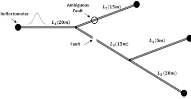
The description of Telegrapher’s equations based models can be found in Clayton [2007]. This kind of model can be used to compute the various signals reflected by a branched network for any Time Domain Reflectometry (TDR) based diagnosis method Auzanneau and Ravot [2007]. 1 represents a complex branched network with an open circuit fault at the distance 25m from the injection point as confirmed by the corresponding reflectogram in Fig.2. Only one reflectometer is placed at the extremity of L1 to diagnose the whole network. The reflectometer
and the network are considered unmatched, explaining the first positive peak on the reflectogram. The end of lines are also unmatched. Here, the detected fault on L3cannot be
distinguished from the same fault on L2.
Fig. 1. Fault location ambiguity in a branched network.
0 20 40 60 80 100 −0.5 0 0.5 1 1.5 Amplitude [V] Distance [m] Healthy network Faulty network Injected Signal Fault
Fig. 2. Reflectogram using TDR method.
In this case, it is possible to add another reflectometer at the end of L2. Although, the ambiguity problem is
resolved for the fault on L3, it would remain inevitable
if another fault appeared on L4. So, another reflectometer
should be added to overcome this ambiguity but with the consequences we know in terms of diagnosis cost. As a so-lution, we propose to introduce the cable life profile aiming at canceling the fault location ambiguity without raising the diagnosis cost. Considering the uncertainty related to fault location, measurement precision and reflectometer reliability, the use of BN seems a suitable candidate to combine these deterministic and stochastic behaviours.
3. BAYESIAN NETWORKS PRINCIPLE
A Bayesian Network (BN, also referred to as belief net-work, probabilistic netnet-work, or causal network) is a mem-ber of the probabilistic Graphical Models (GM) family, known as Directed Acyclic Graph (DAG) Verron et al. [2008]. It is represented by two sets: the set of nodes (qualitative part) and the set of edges (quantitative part) Knox and Mengshoel [2009]. The nodes represent variables of interest, noted as Xi. The edges represent direct
de-pendences among these variables. An arrow from node Xi to Xj represents a probabilistic relation between the
corresponding values where Xi is defined as a parent (or
ascendant) of Xj and similarly Xj is referred to as a child
(or descendant) of Xi. Following the above discussion,
the BN B is defined by a pair B = {G, Θ} where G is the DAG whose nodes X1, X2, · · · , Xn represent
vari-ables of interest and for which edges represent the direct dependencies between them. The parameter Θ denotes the set of parameters of the network which contains the parameter θxi|πi = PB(xi|πi) for each realization xi of
Xi conditioned on πi. Then, the BN B defines a joint
probability distribution over a set of variables of interest where: PB(X1, X2, · · · , Xn) = n Y i=1 PB(Xi|πi) = n Y i=1 θXi|πi. (1)
4. PROPOSED DIAGNOSIS PROCEDURE FOR AMBIGUITY CANCELLATION
The procedure of the proposed diagnosis is shown on Fig.3.
Fig. 3. Diagnosis Procedure in Wiring Networks
First, the complex wiring network is divided into sub-networks where each sub-network is diagnosed at least by one reflectometer. Second, each reflectometer performs the local diagnosis in each sub-network based on the observed symptoms and calculates the conditional probabilities on each branch of the sub-network using BNs. Here, the cable life profile is considered to compute the probability of the presence of the detected fault on each cable. This procedure permits to locate the fault on the sub-network with a reduced uncertainty. Then, the diagnosis system performs the global diagnosis in the whole network by merging the previously defined sub-systems results to locate the fault in the whole network.
19th IFAC World Congress
Table 1. Variables of interest of local diagnosis modelling
Classification Variable Notation Description
Reflectometer EmissionReliability X1∈ χh Reliability of the reflectometer in terms of signal
injection.
ReceptionReliability X2∈ χh Reliability of the reflectometer in terms of signal
reception. Diagnosis Method
MeasurementPrecision X3∈ χh Accuracy of the obtained measurement.
Attenuation X4∈ χh Attenuation of the test signal during its propagation.
Bandwidth X5∈ χo Bandwidth of the channel ( The wider the Bandwidth,
the narrower the peak.)
Cable
ChannelNoise X6∈ χh Noise level in the cable. It impacts on the reflected
signal reception and the measurement precision.
CableLength X7∈ χo Length of the cable. It impacts on the attenuation of
the test signal
CableAge X8∈ χo Age of the cable. It impacts on the fault characteristic.
CableType X9∈ χo Type of the cable. It impacts on the noise on the cable,
the length, the attenuation and the corresponding bandwidth.
Environment Temperature X10∈ χo Exposure of the cable to a heat source promotes its
aging and increases its noise level.
Chafing X11∈ χo Chafing causes the cable aging.
Diagnosis Procedure SignalInjection X12∈ χo Injection of a test signal into the cable network.
RSignalReception X13∈ χo Reception of a reflected signal at the injection port.
Fault PeakPresence X14∈ χo Each impedance discontinuity (fault or junction) is
identified by a peak in the corresponding reflectogram.
FaultonBranch X15∈ χr Detected fault exists in the studied branch.
4.1 Local Diagnosis based on Bayesian Networks
Here, we propose to decompose the diagnosis system into simple sub-systems and model them individually in order to reduce the system complexity Przytula Wojtek and Thompson [2000]. A BN is modelled for each cable tak-ing into account its life profile. The variables of interest, represented in the BN by nodes, are summarized in Table 1. They are classified into groups: reflectometer, diagno-sis method, cable, environment, diagnodiagno-sis procedure and fault. These groups depend on each other and may impact on the fault diagnosis results. In fact, the reflectometer’s reliability in terms of injection or reception impacts on the fault characterisation. For example, in the case of an unreliable reflectometer, an erroneous test signal may be injected. Then, a false interpretation of the reflectogram is made involving unnecessary intervention. Moreover, the choice of the diagnosis method is crucial since some meth-ods being more robust than others to the interference and noise presence such as mutli-carrier methods Ben Hassen et al. [2013], Lelong and Olivas [2009]. In addition to that, the cable’s characteristics (type, age, length, noise) impact on the test signal behaviour during its propagation. For example, a Shielded Twisted Pair (STP) or a coaxial cable is more robust to external electromagnetic interference and cross-talk than an Unshielded Twisted Pair (UTP). Furthermore, the environmental stress (temperature, vi-bration, moisture, etc.) promotes the appearance of cable weaknesses or aging. Taking all these parameters, referred to as cable life profile, into account permits to characterize the fault location uncertainty and then, cancel the ambi-guity problem.
In this case, BN’s variables are divided into three sets which are:
• χr set of nodes representing the real state of the
studied system.
• χhset of nodes representing the hidden symptoms of
the studied system.
• χo set of nodes representing the observed symptoms
of the studied system.
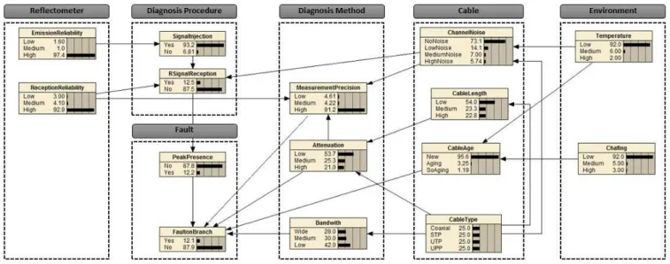
Fig.4 represents the BN dedicated to local diagnosis. It permits to locate the fault on each branch. Let us note that probabilities are given by an expert in the proposed BN. For each reflectometer, the conditional probability on each branch is given by:
P (X15/X3, X4, X5, X8, X14) =
P (X15; X3, X4, X5, X8, X14)
P (X3, X4, X5, X8, X14)
. (2)
where P (X15; X3, X4, X5, X8, X14) represents the joint
probability and P (X3, X4, X5, X8, X14) represents the a
priori probability.
The same process is repeated for all reflectometers imple-mented in the target network.
4.2 Global Diagnosis using Bayesian Networks
In this step, we integrate the results obtained by each reflectometer on each cable in a global BN to locate the fault in the whole network. The variables of interest are summarized in Table 2. The conditional probability related to the presence of the fault on the branch m depends on the gathered information from the reflectometers. This information is obtained by the local diagnosis previously established related to reflectometer Ri and Rj. It is given
as follows:
P (Ym/Yi,m, Yj,m) =
P (Ym; Yi,m, Yj,m)
P (Yi,m, Yj,m)
. (3)
In order to prove the efficiency of the proposed approach, simulation results are presented in the next section.
Fig. 4. Bayesian Network dedicated to local diagnosis on each cable Table 2. Variables of interest of the Global
Bayesian Network
Variable(s) Modality Notation Description
RiF aultonBm Yes/No Yi,m Presence of the fault on
branch Bm according
to the reflectometer i.
RjF aultonBm Yes/No Yj,m Presence of the fault on
branch Bm according
to the reflectometer j.
F aultonBm Yes/No Ym Presence of the fault on
branch Bm.
Fig. 5. A simplified CAN bus
5. SIMULATION RESULTS
Controller Area Network (CAN) bus is widely used in automotive, aircraft, energy distribution, etc., as a mean for enabling robust serial communication between several embedded functions. In this work, a simplified CAN bus is considered where three reflectometers R1,R2 and R3
are used for the diagnosis of the whole network as shown on Fig.5. Here, an Unshielded Twisted Pair (UTP) is considered. The network is made of a main bus whose length is 40m and 6 transmissions lines whose lengths are equal to 2.5m to link the electronic boards to the bus. They are represented by Bi0 where i ∈ {1, 2, · · · , 6}. The extremities of the bus are loaded by 120Ω loads to avoid interference and multi-path fading. The main CAN bus is divided into multiple sections called B1 to B7. An open
circuit fault is simulated on branch B3 at distance 4.5m
from R1, 11.5m from R2and 22.5m from R3. TDR method
is used for the network diagnosis. The idea is to inject,
periodically, a Gaussian pulse signal into the network with an amplitude equal to 1V. Then, the measured signal is basically made of multiple copies of this signal delayed in time. For each copy, the delay is the round trip time necessary to reach the impedance discontinuity from the reflectometer. Given the propagation velocity, it is possible to locate the discontinuity. Although TDR is simple to implement, it suffers from noise weaknesses and signal attenuation as shown on Fig.6 and Fig.7. For reflectometer
−2 −1 0 1 2 3 4 5 6
−0.5 0 0.5 1
1.5 The obtained reflectogram by R1
Amplitude [V] Distance [m] Healthy network Faulty network −2 −1 0 1 2 3 4 5 6 −0.2 0 0.2 0.4 Amplitude [V] Distance [m] Injected Signal Junction1 Fault detection at 4.5 ±0.3m from R1
The difference between healthy and faulty reflectograms
Fig. 6. Fault detection at distance 4.5 ± 0.3m from R1
R1, the fault on Branch B3cannot be distinguished from a
possible fault on B2as shown by the corresponding
reflec-togram in Fig.6. Moreover, it cannot be distinguished from a possible one on branch B30 or B6 for reflectometer R2
as shown by Fig.7. Moreover, it can not be distinguished from a fault on branch B03 for R3. Supposing that cable
B3 is submitted to aggressive thermal stress (near to a
hot unit), it can age quicker and become faulty due to the cable insulation chafing. This knowledge is integrated in the proposed BN presented in Fig.4 and then propagated into the network. This thermal stress is the origin of noise whose amplitude N is given by N (dBW ) = 10 log(kT B) where k is the Boltzmann constant (k = 1.38e−23 J/K), T is the temperature (K) and B is the bandwidth (Hz). The increase of the temperature T causes not only the
0 2 4 6 8 10 12 0
0.5 1
The obtained reflectogram by R
2 Amplitude [V] Distance [m] Healthy network Faulty network 0 2 4 6 8 10 12 −0.1 0 0.1 0.2 Amplitude [V] Distance [m] Injected Signal Junction 1 Junction 2
The difference between faulty and healthy reflectograms
Fault detection at
11.5±0.3m from R2
Fig. 7. Fault detection at distance 11.5 ± 0.3m from R2
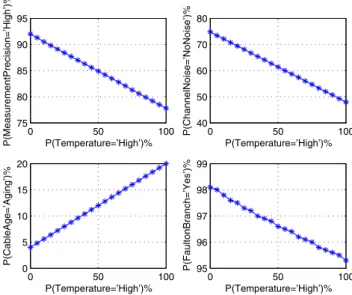
channel noise and cable aging increase, but also the mea-surement precision decrease as shown on Fig.8. This latter is demonstrated by the uncertainty related to the fault position. For example, for R1, the fault is located at
4.5±0.3m from the injection point. These probabilities are obtained for P(X9=’UPP’)=100%, P(X14=’Yes’)=100%,
P(X4=’Low’)=100% and P(X5=’Wide’)=100%.
More-over, that thermal noise may increase the uncertainty related to the fault presence and then trigger false alarms. In this work, all the cables have the same characteristics in terms of impedance, propagation velocity, etc.
As described previously on Fig.3, the diagnosis procedure
0 50 100 75 80 85 90 95 P(MeasurementPrecision=’High’)% P(Temperature=’High’)% 0 50 100 40 50 60 70 80 P(ChannelNoise=’NoNoise’)% P(Temperature=’High’)% 0 50 100 0 5 10 15 20 P(CableAge=’Aging’)% P(Temperature=’High’)% 0 50 100 95 96 97 98 99 P(FaultonBranch=’Yes’)% P(Temperature=’High’)%
Fig. 8. The Temperature impact on the measurement precision, cable age, channel noise and fault location.
includes two steps: local and global diagnosis. In local diagnosis, each reflectometer calculates the conditional probability of the presence of the fault on each branch using equation (2). For simplicity, we present some inter-esting results as shown on Tables 3,4 and 5.
If we look at the results for the local diagnosis, we tend to conclude that the fault is on the branch B2 for
reflectometer R1 as P (X15 =‘Yes’)=91.9% on B2 and
P (X15 =‘Yes’)=89.8% on B3. This ambiguity is caused
Table 3. R1: Local diagnosis dedicated to B3
Symptom Probability Result Probability
P (X10=‘High’)=100 % P (X15=‘Yes’)=89.8% P (X6=‘NoNoise’)=55.9 % P (X3=‘Low’ )=6.33 % P (X8=‘New’ )=80 % P (X14=‘Yes’ )=100 %
Table 4. R1: Local diagnosis dedicated to B2
Symptom Probability Result Probability
P (X10=‘Low’)=100 % P (X15=‘Yes’)=91.9% P (X6=‘NoNoise’)=82.9 % P (X3=‘Low’ )=2.88 % P (X8=‘New’ )=96 % P (X14=‘Yes’ )=100 %
Table 5. R1: Local diagnosis on B30 and B6
Symptom Probability Result Probability
P (X10=‘Low’)=100 % P (X15=‘Yes’)=0.09% P (X6=‘NoNoise’)=82.9 % P (X3=‘Low’ )=2.88 % P (X8=‘New’ )=96 % P (X14=‘Yes’ )=0 %
by the presence of the thermal noise stress on B3 that
impacts badly on the measurement precision and then the fault location. Therefore, we do not limit our study to local diagnosis, as is usually done in conventional methods, but we propose to gather the obtained information by each reflectometer in a global diagnosis.
In the global diagnosis, the results obtained by each diagnosis system on each branch are integrated in a global BN. Fig9 shows that the probability of the presence of the fault on branch B3 is equal to 91.6% and is obtained as
follows:
P (YB3/YR1,B3, YR2,B3, YR3,B3) =
P (YB3; YR1,B3, YR2,B3, YR3,B3)
P (YR1,B3, YR2,B3, YR3,B3)
. (4)
Fig. 9. Global Diagnosis Modelling on B3.
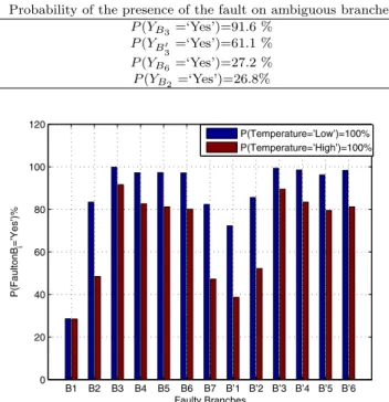
The same process is applied for all the branches of the network. Here, we are interested only by the ambiguous branches B3, B2, B5 and B30. Table 6 summarizes the
probability of the presence of the fault in each of them. Based on the obtained probabilities, we may conclude that the fault is on branch B3 with probability 91.6 %.
The proposed two-stages approach is applied in each branch of the bus CAN as shown on Fig.10. It is obvious that the fault on B1 is located with high uncertainty as
R2 and R3 do not detect it due to its distance from these
reflectometers. Moreover, the thermal stress influences badly on the fault location.
Table 6. Global Diagnosis for Fault Location
Probability of the presence of the fault on ambiguous branches P (YB3 =‘Yes’)=91.6 % P (YB0 3 =‘Yes’)=61.1 % P (YB6 =‘Yes’)=27.2 % P (YB2=‘Yes’)=26.8% B1 B2 B3 B4 B5 B6 B7 B’1 B’2 B’3 B’4 B’5 B’6 0 20 40 60 80 100 120 Faulty Branches P(FaultonB i =’Yes’)% P(Temperature=’Low’)=100% P(Temperature=’High’)=100%
Fig. 10. Fault location probability in each branch of the CAN bus.
Simulation results demonstrate that the introduction of life profile cable permits to efficiently diagnose the network at a low cost (only 3 reflectometers are implemented). Moreover, it permits to reduce the uncertainty related to fault location in complex wiring network. One can notice that the reliability of the reflectometer in emission and reception is considered in the obtained statistics. This reliability differs from a reflectometer to another and impacts on the fault location. In this paper, all reflectometers R1, R2 and R3are considered reliable with
P (X1=‘High’)=97.4% and P (X2=‘High’)=92.4% for R1,
P (X1=‘High’)=96.4% and P (X2=‘High’)=91.4% for R2
and P (X1 =‘High’)=96.2% and P (X2 =‘High’)=91.3%
for R3. A deep study on the reflectometers reliability and
its impact on the obtained results will be the purpose in further works.
6. CONCLUSION
In this paper, a new strategy based on the cable life profile has been proposed for the diagnosis of complex topology wiring networks, and applied to a CAN bus. Our main objective was to find a good compromise between the system cost (diagnosis systems number) and the diagnosis quality. Here, the use of BNs was motivated by the uncer-tainty regarding diagnosis system reliability, measurement precision, and wire faults characterization. The proposed strategy includes two steps: (1) local diagnosis based on BNs, (2) global diagnosis for the whole network to locate the detected fault(s). In local diagnosis, each reflectometer introduces the cable life profile to calculate the condi-tional probability of the presence of the fault on each branch. Then, the obtained results for each reflectometer are integrated into a global BN to locate the fault in the whole network. Simulation results prove the efficiency of the proposed strategy to help cancel the ambiguity for
fault location in a branched network. In this context, a deep study on the reflectometers reliability and its impact on the obtained results will be the purpose in further works. In addition to that, other influential factors (such as chafing, attenuation, bandwidth, etc.) may affect the diagnosis quality and then should be also considered. Fi-nally, in-depth works based on experience feedback would improve the conditional probabilities tables quality thanks to learning Bayesian Networks.
REFERENCES
F. Auzanneau. Wire troubleshooting and diagnosis: Re-view and perspective. Progress In Electromagnetics Research B, 49:253–279, 2013.
F. Auzanneau and N. Ravot. Defects detection and localization in complex topology wired networks. Annals of Telecommunications, 62:193–213, Feb 2007.
W. Ben Hassen, F. Auzanneau, F. Peres, and A. Tchangani. OMTDR using BER Estimation for Ambiguities Cancellation in Ramified Networks Diagnosis. In IEEE ISSNIP Conference, Melbourne, Australia, April 2013.
R. P. Clayton. Analysis of Multiconductor Transmis-sion Lines. Special Issue of IEEE Transactions on Instrumentation and Measurement, 2007. ISBN-13: 978-0470131541.
W. Ben Hassen, F. Auzanneau, F. Peres, and A. Tchangani. A Distributed Diagnosis Strategy using Bayesian Network for Complex Wiring Networks. In IFAC Workshop on Advanced Maintenance Engineering, Services and Technology (AMEST), 2012.
W. Ben Hassen, F. Auzanneau, F. Peres, and A. Tchangani. Optimisation de capteurs de diagnostic de defauts par reflectometrie dans les reseaux filaires complexes en utilisant les reseaux bayesiens. In Qualita, Compiegne, France, March 2013a.
W. Ben Hassen, F. Auzanneau, F. Peres, and A. Tchangani. Diagnosis Sensor Fusion for Wire Fault Location in CAN Bus Systems. In IEEE SENSORS, pages 1–6, Baltimore, Maryland, USA, November 2013b.
W. Bradley Knox and Ole Mengshoel. Diagnosis and Reconfiguration using Bayesian Networks: An Electrical Power System Case Study. In IJCAI 2009 Workshop on Self-* and Autonomous Systems, 2009.
A. Lelong and M. Olivas. On Line Wire Diagnosis using Multicarrier Time Domain Reflectometry for Fault Location. In IEEE Sensors Conference, pages 751–754, October 2009.
K. Przytula Wojtek and D. Thompson. Construction of Bayesian networks for diagnostics. In IEEE Aerospace Conference, volume 5, pages 193–200, 2000.
S. Verron, P. Weber, D. Theilliol, T. Tiplica, A. Kobi, and C. Aubrun. Using Bayesian networks for decision in the simultaneous faults case. In Workshop on Advanced Control and Diagnosis (ACD’08), Coventry, Royaume-Uni, 2008.
E. Villeneuve, C. Beler, F. Peres, and L. Geneste. Hy-bridization of Bayesian Networks and Belief Functions to Assess Risk. Application to aircraft Disassembly. In-ternational Conference on Industrial Engineering and Systems Management (IESM), 2011.