To link to this article: DOI:10.1155/2015/538643
http://dx.doi.org/10.1155/2015/538643
This is an author-deposited version published in:
http://oatao.univ-toulouse.fr/
Eprints ID:
15553
To cite this version:
Ben Hassen, Wafa and Auzanneau, Fabrice and Incarbone, Luca and
Pérès, François and Tchangani, Ayeley Distributed sensor fusion for wire
fault location using sensor clustering strategy. (2015) International
Journal of Distributed Sensor Networks, 2015. pp. 1-17. ISSN 1550-1329
O
pen
A
rchive
T
oulouse
A
rchive
O
uverte (
OATAO
)
OATAO is an open access repository that collects the work of Toulouse researchers and
makes it freely available over the web where possible.
Any correspondence concerning this service should be sent to the repository
administrator:
[email protected]
Distributed Sensor Fusion for Wire Fault Location
Using Sensor Clustering Strategy
Wafa Ben Hassen#1, Fabrice Auzanneau #2, Luca Incarbone #3, François Pérès ∗3 and Ayeley P. Tchangani ∗4,
# CEA, LIST, Laboratoire de Fiabilisation des Systèmes Embarqués, F-91191 Gif-sur-Yvette, France ∗LGP, ENIT, INPT, Université de Toulouse, F-65016 Tarbes, France.
Abstract
From reflectometry methods this work aims at locating accurately electrical faults in complex wiring networks. Increasing demand for on-line diagnosis has imposed serious challenges on interference mitigation. In particular, diagnosis has to be carried out while the target system is operating. The interference becomes more even critical in the case of complex networks where distributed sensors inject their signals simultaneously. The objective of this paper is to develop a new embedded diagnosis strategy in complex wired networks that would resolve interference problems and eliminate ambiguities related to fault location. To do so, OMTDR (Orthogonal Multi-tone Time Domain Reflectometry) method is used. For better coverage of the network, communication between sensors is integrated using the transmitted part of the OMTDR signal. It enables data control and transmission for fusion to facilitate fault location. In order to overcome degradation of diagnosis reliability and communication quality, we propose a new sensor clustering strategy based on network topology in terms of distance and number of junctions. Based on CAN bus network, we prove that data fusion using sensor clustering strategy permits to improve the diagnosis performance.
Index Terms
Embedded diagnosis, complex wiring network, reflectometry, sensor fusion, ambiguity, clustering.
I. INTRODUCTION
I
N the era of Internet of Things, the presence of wired networks remains a fundamental pillar for the transmission of electric energy or information. Whether they are used in aerospace, automotive, telecommunications or even energy distribution, cables are victims of their environment. In fact, they often face aggressive conditions such as mechanical vibration, thermal stress, moisture penetration, etc. These conditions cause the appearance of faults with different severity levels ranging from a simple fissure in the cable sheath to the crack of the cable. This has led to several researches related to diagnosis methods for fault detection and location such as X-Ray, visual inspection, infrared thermal imaging, continuity measurement, etc [1]. Moreover, the complexity of wired networks has increased due to the appearance of the “X-by-Wire” technology, replacing mechanical and hydraulic components by programmable electronic systems for steering, braking, suspension, etc. This trend is also present in avionics known as “Fly-by-Wire” where the embedded electrical power has moved from 320 kilo Watts (kW) in an Airbus 320 to 800 kW in an Airbus 380. The increasing number of embedded electronic systems has led to the increase of the length of the cables that connect them: up to 530 km in an Airbus 380. Indeed, the increase of the complexity of wired networks leads to the increase of the difficulty of their maintenance that becomes not only problematic but also expensive. The loss in efficiency of maintenance may result in the appearance of serious faults in cables.Cable faults can have tragic consequences when the cables are part of critical systems such as aircrafts, nuclear plants, etc. For example, cables have been considered responsible for the crash of TWA Flight 800 (1996) and Swissair 111 (1998). This has led to the need of permanent diagnosis for detecting and locating the first signs of weakness in the cables as soon as possible in order to avoid dramatic accidents. This need for a permanent diagnosis involves the integration of the diagnosis function in the system where wired networks operate, called embedded diagnosis [2]. It implies serious constraints related to the diagnosis performance optimization (i.e. fault location precision), integration difficulty and the diagnosis system (or sensor) reliability. To do so, the most appropriate method is reflectometry. It consists in injecting a test signal at an extremity of the wired network under diagnosis. This signal propagates along the network and each impedance discontinuity encountered (junction or fault) sends a part of its energy back to the injection point. Finally, the analysis of the reflected signal permits to detect, locate and determine the nature of the fault(s).
The interest of the embedded diagnosis is that it performs network diagnosis concurrently to the normal operation of the target network (i.e. communication, energy distribution, etc.). This is called online diagnosis. This implies additional constraints related to the diagnosis harmlessness [3]. In fact, test signals must not interfere with the useful signals. To do so, the choice of the injected signals must be judicious to avoid the frequency bands used by the target system and called prohibited bandwidth. In the literature, several methods have been proposed to resolve interference problems such as Sequence Time Domain Reflectometry (STDR) [4], Spread Spectrum Time Domain Reflectometry (SSTDR) [5], Noise Domain Reflectometry
(Noise Domain Reflecometry) [6] and Multi-Carrier Time Domain Reflecometry (MCTDR) [7]. Recently, a new method called Orthogonal Multi-tone Time Domain Reflecometry (OMTDR) has been proposed [8]. It applies the principles of Orthogonal Frequency Division Multiplexing (OFDM) to wired network diagnosis. The idea is to divide the bandwidth into multiple sub-bands using orthogonal and then overlapped sub-carriers which permits to maximize the spectral efficiency and total spectrum control. Then, the prohibited frequency band may be avoided by canceling the corresponding tone of the OMTDR signal.
Even if reflectometry has proven its efficiency in detecting and locating faults in simple wired networks (i.e. transmission line), it may suffer from ambiguity problems in the case of complex wired networks. In fact, using a single sensor is no longer possible to cover the whole network. This may be explained by the signal attenuation due to the traveled distance and multiple junctions. Although the distance between the injection point and the fault may be determined, the identification of the faultive branch remains ambiguous. As a solution, a distributed diagnosis is used. The idea is to implement several sensors at different extremities of the network in order to maximize the diagnosis coverage. However, as multiple sensors are making measurements simultaneously, specific signal processing methods are required to avoid interference between concurrent sensors [9], [10]. To do so, we propose a new sub-carriers allocation method using OMTDR reflectometry. This solution permits to offer the same perspective of the network to all the sensors and then enhance the diagnosis reliability.
In the context of distributed diagnosis, we propose to integrate communication between sensors via the transmitted part of the test signal which has never been done with conventional methods [9], [10]. For this reason, the test signal must be capable of carrying information which is the case of OMTDR method [11]. The fusion of all this information, based on master/slave protocol, provides unambiguous location of the fault in complex wired networks. Moreover, it may provide information about the health state of the sensors in the network. However, we may also be facing diagnosis reliability and communication quality degradation due to the signal attenuation during its propagation. As a remedy, we propose a new sensor clustering strategy based on the distance and number of junctions. The data fusion using sensor clustering permits to improve the diagnosis performance in complex wiring networks.
The remaining of this paper is organized as follows. In section II, wiring fault diagnosis using reflectometry is introduced. In section III, OMTDR method is described. Even if OMTDR has proven its efficiency in simple topology, it may suffer from ambiguity problems in complex wiring networks as shown in section IV. As a solution, distributed diagnosis is applied. However, this imposes serious challenges related to interference mitigation. For this reason, we propose in section V, a new sub-carrier allocation method using OMTDR method. After interference mitigation, we propose in section VI to integrate communication between sensors based on OMTDR method to enable data fusion. In the case of complex wiring networks, we propose in section VII a sensor clustering strategy based on the distance and number of junctions in the network. Finally, experimental results are presented in the next section in order to evaluate the performance of the proposed strategy using real signals.
II. WIRING FAULTS DIAGNOSIS USING REFLECTOMETRY
For many years, a wire has been considered as a system that could be installed and run for the life of the system in which it operates. However, this practice has rapidly changed with the observation that wires are victims of wear and can experience some failures. These failures can cause the appearance of serious faults such as loss of electrical signal, distortion of information, system malfunction, smoke, fire, etc. Unfortunately, these faults can have dramatic consequences if the wires are part of critical systems. Based on collected data by the Air Force Safety Agency (AFSA) between 1989 and 1999, cables are responsible for many accidents in aircraft [12], [13]. The problems in the cables can also implies huge costs. In 2004, the US Navy had to abort more than 1400 missions because of wiring problems and keep about 2% to 3% of its fleet grounded for the same reasons [1]. The cost of maintaining an aircraft on ground was estimated by several airlines at 150 000 dollars per hour. In fact, the most frequent causes of fault appearance are: insulation aging, mechanical stress, thermal stress, moisture, etc. According to NASA [14], 80% of faults are caused by human intervention. Indeed, a maintenance operator may have to use cables as ladders to reach inaccessible areas during maintenance operation. These factors cause considerable changes in the intrinsic parameters of the cable and result then in the appearance of faults. Depending on their severity, faults in cables can be divided into two major groups: hard faults and soft faults. On the one hand, hard faults are characterized by an interruption of the energy or information circulation in the damaged cable. They include open circuit and short circuit. On the other hand, soft faults result in a small variation in the characteristic impedance of the cable caused by sheath crack, conductor degradation, etc. These faults do not always lead to catastrophic incident as they do not interrupt energy or information circulation, but can generate hot spots and hard faults in over the long term due to mechanical stress, moisture penetration, thermal stress or even cable aging. An efficient diagnosis system is mandatory to detect and precisely locate the fault(s).
In this context, various methods have been studied such as: visual inspection, X-Rays, capactive and inductive methods, reflectometry, etc. While the visual inspection is commonly used, it is inefficient in complex wired networks. It can detect
only 25% of faults present in an aircraft [14] when a large portion of the wired network is hidden by huge structures such as electric panels, components or other cables. The X-Ray inspection requires the use of heavy equipment, direct access to cable and human intervention for data analysis. Both methods, capacitive and inductive, are efficient in the case of of point-to-point cable diagnosis, but remain limited in the case of complex wired networks. In addition, they can be used only if the cable is off-line. Table II summarizes the main advantages and disadvantages of those methods. Among all known diagnosis methods, reflectometry appears to be the most promising one.
Table I
COMPARISON OF DIAGNOSIS METHODS: , THE METHOD DETECTS THE FAULT. - THE METHOD DETECTS THE FAULT UNDER CONDITIONS. / THE METHOD DOES NOT DETECT THE FAULT.
Visual inspection
X-Rays Capacitive and inductive methods Frequency Domain Reflectometry Time Domain Reflecometry
Long cable (i.e. >30
m)
/
/
-
,
,
Buried cable/
/
-
,
,
Soft fault-
,
/
-
-Intermittent fault/
/
/
-
-Online diagnosis/
-
/
,
,
Complex network/
/
/
/
-Reflectometry includes two main families: Time Domain -Reflectometry (TDR) and Frequency Domain -Reflectometry (FDR). On the one hand, TDR injects periodically a probe signal and the reflected signal is basically made of multiple copies of this signal delayed in time. For each copy, the delay is the round trip time necessary to reach the discontinuity from the injection point. This signal is called “reflectogram” [15]. So, the knowledge of the propagation velocity and the time delay of each copy permits to locate the corresponding impedance discontinuity. On the other hand, FDR injects a set of sine wave called chirp [16], [17], [18]. Then, the analysis of the standing wave permits to give information about the fault location. This analysis becomes difficult to interpret in the case of complex wiring network. For this reason, TDR is more interesting than FDR in complex wiring networks.
III. ORTHOGONALMULTI-TONETIMEDOMAINREFLECOMETRY
The multi-carrier modulation Frequency Division Multiplexing (FDM), used by reflectometry MCTDR, divides the bandwidth into several sub-bands using sub-carriers. These sub-carriers must be separated by a guard band to avoid interference problems. This leads to non optimal use of the available bandwidth. Indeed, up to 50% of the bandwidth is used by the inter-band intervals [19], [20]. Orthogonal Frequency Division Multiplexing (OFDM) is an interesting modulation technique permitting to reduce those guard intervals and then bandwidth loss. This technique is well-known in the fourth generation cellular networks such as Long Term Evolution (LTE), Worldwide Interoperability for Microwave Access (WiMAX) 802.16, etc, thanks to its capacity to achieve a very high data rate transmission. The idea is to divide the total bandwidth using orthogonal and then overlapped sub-carriers which permits to maximize the spectral efficiency and interference mitigation.
A. Modeling and functional description of OMTDR signal
The OFDM technique consists in dividing the bandwidth B using N sub-carriers modulated independently by a Quadrature Amplitude Modulation with M states (M-QAM). The M-QAM modulation is a digital modulation that changes the amplitude
and the phase of each sub-carrier according to binary information to be transmitted on it. In the OMTDR method, the test signal injected down the wiring network is defined as:
sk(t) = N −1
∑ n=0
Sk,ngn(t− kTs) . (1)
where n is the sub-carrier number in the considered OFDM symbol k. Each sub-carrier signal gn(t) is modulated independently by the complex valued modulation symbol Sk,n and is expressed as:
gn(t) = {
ej2πn∆f t if t ∈[0, Ts] .
0 if not. (2)
where Ts = 1/∆f represents the useful OFDM symbol duration. ∆f is the frequency distance between two consecutive sub-carriers. The spectrum of the test signal Sk(f) is given by:
Sk(f) = Ts N −1
∑ n=0
Sk,nsinc(πTs(f− n∆f)) . (3)
where sinc(x) = sin(x)/x. The injected signal xk(t) is obtained by a digital-to-analog conversion (DAC) and correspond to the following relation:
xk(t) = +∞ ∑ k=−∞ N −1 ∑ n=0 Sk,nej2πn∆f tΠ(t− kTs). (4)
where Π is the shaping filter and is given as follows:
Π(t) = { 1 if t ∈[0, Ts].
0 if not. (5)
The auto-correlation function of the test signal gives an idea about the observed shape at each peak related to the impedance discontinuity. In the OMTDR method, it is expressed as follows:
Css(τ) = 1 N N −1 ∑ i=0 sk,is ∗ k,i−τe −j2πτ n N. (6)
where τ is the delay and N is the number of samples. Indeed, the test signal sk(t) is sampled with the sample interval ∆t = 1/N∆f in numerical applications. Here, the sample of the transmit signal is denoted by sk,i where i ∈{0, 1,⋯, N − 1} and is expressed as follows:
sk,i= N −1 ∑ n=0 Sk,nej2πi n N. (7)
Fig.1 shows the auto-correlation function of the OMTDR signal (6). The auto-correlation function is a pulse consisting of a central lobe and side lobes. The presence of side lobes may cause a fault detection problem (false alarm).
−100 −80 −60 −40 −20 0 20 40 60 80 −0.2 0 0.2 0.4 0.6 0.8 1 Samples Normalized Amplitude
Online diagnosis provides the possibility of performing the diagnosis concurrently to the normal operation of the network. However, it imposes serious challenges related to Electro-Magnetic Compatibility (EMC) constraints. When the energy of the test signal should be limited in some frequency bands, the corresponding coefficients Sk,n must be canceled as follows:
Sk,n= 0 ⇒ Sk(n∆f) = 0, where n ∈ [0, N− 1] and n ∈ N. (8) The signal xk(t) given by equation (4) is injected into the line and is reflected if it meets one or more impedance discontinuities during its propagation.
B. Analysis of the measured signal using OMTDR method
The received signal is represented as the convolution between the test signal and the channel impulse response hk(t) in the presence of Additive White Gaussian Noise (AWGN). At the output of the analog-digital converter, the received signal is sampled at the rate 1/T s. We can write the following relation:
yk,i= sk,i∗ hk,i+ nk,i. (9)
The reflected signal y
k = (yk,0, yk,1, ⋯, yk,N −1) is now correlated with the test signal sk = (sk,0, sk,1, ⋯, sk,N −1) and the obtained signal is given as follows:
rsyk(τ ) = 1 N N −1 ∑ i=0 sk,iyk,i−τ∗ . (10)
In online diagnosis, the modifications of the OMTDR signal spectrum to fulfill the EMC requirements lead to information loss. Indeed, in the frequency domain, the network response is clearly unknown in the canceled frequency bands. To verify this, we take the example of a transmission line of length 100 m with a soft fault at 50 m from the injection point and an open circuit at its end. Here, 50% of the bandwidth is canceled. We note that the loss of information causes the appearance of distortions around the peaks as shown in Fig.2.
50 100 150 200 −0.2 −0.1 0 0.1 0.2 0.3 0.4 0.5 Distance (m) Normalized Amplitude
Figure 2. Obtained reflectogram where samples{0, 1, ⋯, 255} are canceled.
The estimation of this missing information requires a specific post-processing. To do so, we propose here to introduce an averaging step for multiple OFDM symbols as follows:
¯ rsy= 1 K K−1 ∑ k=0 rsyk. (11) where rsy
k is the signal obtained from equation (10) after correlation between test signal and reflected signal in symbol OFDM
k. K represents the number of OFDM signals. Note that generated bits are different from an OFDM symbol to another. Fig.3 shows the obtained reflectogram after averaging 10 measures.
As mentioned above, the presence of side lobes (Fig.1) is unsuitable to detect and locate soft faults mainly in complex wiring networks. To improve the analysis of the reflectogram, we propose to introduce a convolution between the measure ¯rsy and a windowing function ω as follows:
ˆ
where i is the sample of the measure i ∈{0, 1, ⋯, N − 1} and i′ is the sample of the windowing function i′
∈{0, 1, ⋯, N′− 1}. N and N′ represent the number of samples of the measure and the windowing function, respectively. The number of samples of the convoluted signal is noted ˆN where ˆN =N + N′
− 1. The Dolph-Chebyshev window seems to be the best window to achieve a good compromise between the width of the central lobe at mid-height and the amplitude of the side lobes [21], [22]. Fig.4 shows the obtained reflectogram after convolution with a Dolph-Chebyshev window where N′=20. Fig. 5 shows the principle of OMTDR reflectometry for online diagnosis.
0 50 100 150 200 250 −0.1 0 0.1 0.2 0.3 0.4 0.5 Distance (m) Amplitude normalisée
Figure 3. Obtained reflectogram after averaging where samples{0, 1, ⋯, 255} are canceled. 50 100 150 200 250 −0.1 0 0.1 0.2 0.3 0.4 0.5 Distance (m) Normalized Amplitude
Figure 4. Obtained reflectogram after post-processing where samples {0, 1, ⋯, 255} are canceled.
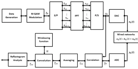
Figure 5. Principle of OMTDR reflectometry for online diagnosis.
IV. FAULTLOCATIONAMBIGUITYPROBLEMS INCOMPLEXBRANCHEDNETWORKS
In complex wiring network, using a single sensor is no longer possible to cover the whole network. This may be explained by the signal attenuation due to the distance and multiple junctions. Although the distance between the injection point and the fault may be determined, the identification of the defected branch remains ambiguous. To illustrate this, Fig.7 shows the computed reflectogram for the branched network of Fig.6 with an open circuit fault at 25 m from the injection point. Only one reflectometer is placed at the extremity of L1to diagnose the whole network. The reflectometer and the network are considered unmatched, explaining the first positive peak on the reflectogram. The end of lines are also unmatched. Here, the detected fault on L3 cannot be distinguished from the same fault on L2. In this case, it is possible to add another reflectometer at the
Figure 6. Fault location ambiguity in a branched network. 0 10 20 30 40 50 60 70 80 90 −0.5 −0.4 −0.3 −0.2 −0.1 0 0.1 0.2 0.3 0.4 0.5 Amplitude [V] Distance [m] Faulty network Junction End of line L 2 Fault
Figure 7. Reflectogram using TDR method.
end of L2using distributed diagnosis.The ambiguity disappears thanks to this new sensor but would recur upon the occurence of a new fault on L4. So, another reflectometer should be added to overcome this ambiguity. Then, distributed reflecometry is a suitable method to overcome ambiguity problems. However, several challenges are imposed related to interference mitigation when all sensors use the network simultaneously. In the context of multi-carrier method, we propose to use Frequency Division Multiple Access (FDMA) method as shown later.
V. A NEWSUB-CARRIERALLOCATIONMETHOD FORINTERFERENCEMITIGATION
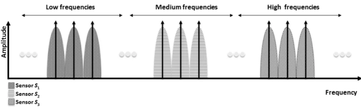
The use of OMTDR signal made of orthogonal subcarriers allows the avoidance of an interference by allocating a different set of available sub-carriers to each sensor. The conventional method is to allocate to each sensor a set of adjacent sub-carriers. Fig. 8 shows a spectrum of OMTDR method whose sub-carriers are divided into three sensors S1, S2and S3. Taking the sub-carriers in ascending values of their central frequencies, a first group (low frequencies) of adjacent sub-sub-carriers (3 sub-sub-carriers in the example in Fig. 8) is allocated to S1. A second group (medium frequencies) of adjacent sub-carriers is assigned to S2. Finally, a third group (high frequencies) of adjacent sub-carriers is allocated to S3. Although adjacent sub-carriers allocation
Figure 8. Example of Adjacent Sub-carriers Allocation
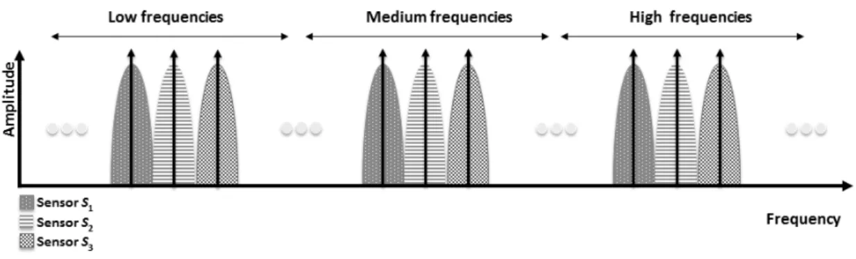
method permits to avoid interference, it has drawbacks. Indeed, in the configuration of Fig.8, S1 uses sub-carriers located substantially at low frequencies, S2 uses sub-carriers located in the medium frequencies and S3 uses sub-carriers located in the higher frequencies. This difference in spectrum causes unfortunately a difference in perspective of the network seen by each sensor. Therefore, the quality of the 3 obtained reflectograms is different in this case. In fact, propagation phenomena (attenuation and dispersion) depend extremely on the signal frequency. So, the attenuation and dispersion is more important in high frequencies than in low frequencies. For all these reasons, adjacent sub-carriers allocation is not efficient in the reflectometry-based wire diagnosis. Thus, we propose a distributed sub-carriers allocation method as shown in Fig.9. In this case, each sensor uses sub-carriers in regularly distributed frequencies and thus, all sensors use signals operating at similar frequencies.
In the example in Fig.9, the sub-carriers are alternately allocated to one of three reflectometers S1, S2and S3. Proceeding in this way, we ensure that each sensor S1, S2and S3will generate a multi-carrier signal using frequencies uniformly distributed
Figure 9. Example of Distributed Sub-carriers Allocation
in the useful band. All generated signals have then a close spectral profile which ensures obtaining homogeneous reflectograms. Three sensors S1, S2 and S3 are implemented in the network shown in Figure 6. S1, S2 and S3 are related, respectively, to branch L1, L2 and L4. Here, the sensors and the branches are considered matched. The branch L5 is affected by an open circuit at its end. Figures 10, 11 and 12 show the obtained reflectograms by sensors S1, S2 and S3 in two cases: allocation of sub-carriers is performed as described in Fig.8 (adjacent allocation) and allocation of sub-carriers is performed as described in Fig.9 (distributed allocation). We remark that the distributed allocation method permits to enhance the quality
10 15 20 25 30 35 40 −0.6 −0.4 −0.2 0 0.2 0.4 0.6 0.8 Distance (m) Amplitude Adjacent Allocation Distributed Allocation Junction Fault on L3
Round−trip on the fault
Figure 10. Reflectogram of S1 0 5 10 15 20 25 30 −0.4 −0.2 0 0.2 0.4 0.6 Distance (m) Amplitude Adjacent Allocation Distributed Allocation Junction Fault on L3
Round−trip on the fault
Figure 11. Reflectogram of S2 5 10 15 20 25 30 35 40 −0.4 −0.2 0 0.2 0.4 0.6 0.8 Distance (m) Amplitude Adjacent Allocation Distributed Allocation Junction Fault on L3 End of line L5 Figure 12. Reflectogram of S3
or high frequencies.
After interference mitigation in distributed reflectometry, we propose now to integrate communication between sensors via the transmitted part of the test signal which has never been done with conventional methods [9], [10]. For this reason, the test signal must be capable of carrying information which is possible thanks to the OMTDR method [11]. The fusion of all this information, based on master/slave protocol, provides unambiguous location of the fault in complex wired networks as shown as follows.
VI. DATA FUSION FOR WIRE FAULT LOCATION
In this section, we propose to integrate communication between sensors to enable data fusion in the context of distributed diagnosis. For this reason, we propose to use not only the reflected part of the diagnosis signal, but also the transmitted part. A signal carrying information is then used as test signal to enable reflectometry measurement and communication through the OMTDR technique. To do so, let’s begin with the structure of the test signal.
A. Frame description
As the test signal is carrying information, the data is formatted into frames themselves subdivided into 9 fields. The frame is delimited by a Start Of Frame (SOF) (8 bits) and an End of Frame (EOF) (8 bits) field. Each sensor is identified in the network by an ID (16 bits). Then, the field CMD (8 bits) reveals the nature of the frame (data or request). The field DLC gives the length of the transmitted data that may vary between 21-53 bytes. Cyclic Redundancy Check (CRC) is used for error detection as shown by Fig.13 and ACK to acknowledge the good receipt of the message.
Figure 13. A frame structure
After having described the frame structure, we propose now to classify the distributed sensor into two groups: master and slave.
B. Classification of sensors
In master/slave protocol, the choice of the master is crucial to ensure the efficiency of the proposed diagnosis strategy. To do so, we propose to assign a weight of eligibility to each sensor for sensor classification. In fact, the reflectogram’s quality depends strongly on the network topology in terms of distance and number of junctions [1]. The same remark holds for the communication quality. We propose now to study the impact of network topology on communication quality. We focus only on the number of junctions in the network. Recall that a junction causes the reflection of a part of the energy of the transmitted signal. Fig.14 shows the different topologies considered in order to calculate the BER. For this, the distance between the transmitter and the receiver is set to 10 m and the SNR is 10 dB. Fig.15 shows the evolution of the BER versus the number of junctions in the network. It may be noted that the BER depends on the complexity of the network topology in terms of junctions number. Indeed, the increase of the number of junctions causes the increase of the attenuation of the signal during its propagation.
Based on these findings, the weight of eligibility may be calculated by the following parameters:
● The sum of distances DSi = ∑Sj∈VSidistance(Si, Sj) between sensor Si and the other sensors Sj, i ≠ j where VSi is
the set of sensors in the network. The minimization of this value reduces the propagation attenuation and hence the bit error rate.
● The number of junctions JSi = ∑Sj∈VSijunction(Si, Sj) between sensor Si and the other sensors Sj, i ≠ j. The
minimization of this value reduces the bit error rate due to multiple reflections as shown by Fig.15. The weight of eligibility for sensor Si is given by:
wSi= DSi× JSi. (13)
In fact, the minimization of the weight of eligibility reduces firstly the bit error rate and increases the diagnosis accuracy since it minimizes the attenuation of the test signal. Then, the sensor with the lowest weight of eligibility is designated as the master while other sensors are considered as slaves. Besides network diagnosis (signal injection, received signal processing, fault detection, etc.), the master must ensure the management of its slaves (synchronization, resource allocation, routing table, etc.), the information collection, data analysis and decision making. For their part, slaves must do their diagnosis, identify the fault position and send it to their master.
Figure 14. Evolution of the topology of the network 0 1 2 3 4 5 0.1 0.2 0.3 0.4 0.5 0.6 0.7 Number of junctions BER (%) 0 junction 1 junction 2 junctions 3 junctions 4 junctions 5 junctions
Figure 15. Evolution of bit error rate in terms of junctions number
C. Automation of fault detection and location
In this section, we propose to develop an algorithm to automate the detection and location of a fault. We propose firstly to generate a reference measurement obtained when the network is healthy. We propose to save in sensor memory only the position of the local extrema of the corresponding reflectogram to avoid the saturation of the embedded memory. The number of extrema in the reference is noted Nref. The set of extrema is ςref = {eref(1), eref(2), ⋯, eref(Nref)}. We characterize each extremum by its position and amplitude as follows: (pref(i), aref(i)) where i ∈ {1, 2, ⋯, Nref}. Fig.16 describes the proposed algorithm for detecting and locating automatically a possible fault. After the construction of the reflectogram, we extract local extrema noted ecurr(pcurr(i), acurr(i)). Then, we compare it in terms of position with those stored in memory (reference). This indicates whether there has been an evolution of the state of the network or not. We note ςcurr ={ecurr(1), ecurr(2), ⋯, ecurr(Ncurr)} where Ncurr is the number of extrema in the current measure. If there is no change, we must ensure that all local extrema are treated. Otherwise, we should treat the following extremum where i ← i + 1. However, if the detected extremum does not belong to the reference set ςref, we must determine whether the amplitude of the extremum value is greater than a threshold noted T to avoid considering noise as a fault. In the presence of AWGN noise, the threshold is expressed as follows:
T = 2N σ2. (14)
where N represents the number of samples and σ the AWGN variance.
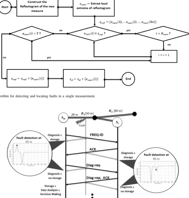
The algorithm described above allows automatic detection and location of a fault in a single reflectometry measurement. Indeed, saving only local extrema permits to optimize both processing time and memory capacity. Thereafter, the position of the detected fault is encapsulated in the field data of the frame to be sent to the master if the actual sensor is a slave. D. Description of the communication protocol
The master noted Sm sends a data message for initialization with CMD=“FREQ-ID” and the data field contains the set of sub-carriers allocated to the slave Ss as seen in section V and shown on the upper part of Fig.17.
Considering a soft fault with ∆Zc= 20% on the branch B1, a part of energy of the message sent by Sm is reflected back. The master Smconstructs the corresponding reflectogram and detects the presence of the soft fault at 20 m from Sm based on the algorithm shown on Fig.16. The soft fault position is stored in the memory of sensor Sm. After receiving the initializing message of its master Sm, the salve Ss injects an OMTDR signal which contains an acknowledge message to Sm where CMD=“ACK” and the filed ACK=“01”. In order to avoid that the data field remains empty (diagnosis precision degradation), a zero padding with at least 21 bytes is done. Here, a part of energy of the message is reflected back and the slave defines the fault position at 90 m based on its reflectogram. This position is also stored in its memory. Note that the processing of the measurement is done locally. For this, the slave must have a good memory and processing capacity.
When master Sm receives the acknowledgment of its salve, a new request message where CMD=“Diag-Req” is sent to Ss for information providing. The sensor must, every time, analyze the new reflectogram and compare it with that obtained at the previous time to check if the fault persists, if it has evolved (amplitude variation, increasing the length, etc) or even if there
Figure 16. Algorithm for detecting and locating faults in a single measurement.
Figure 17. Scenario of the communication protocol
is another fault that appeared in the meantime, etc. The slave Ss sends a data message where CMD=“Diag-Req” containing the information about the fault position. At the reception, the master Sm extracts the data sent by its slave and stores it in its memory. After receiving data sent by all its slaves, the master analyzes this data and makes the decision about the fault location in the network. In this example, the fault is located on branch B1 as shown by Fig.17.
The data fusion, based on master/slave protocol, provides unambiguous location of the fault in complex wired network. Moreover, it may provide information about the state (i.e. out of service) of the sensors in the network. We propose to verify the efficiency of data fusion strategy in a CAN bus system.
E. Validation of the strategy in a CAN Bus system
In this section, we consider the CAN bus system described in Fig.18. The network consists of six sensors Si, i ∈{1, 2, ⋯, 6} with the same characteristics (homogeneous network). These sensors are considered matched with the network cables where Zc= 120Ω. The bus is divided into multiple portions noted from B1to B7with lengths 5 m, 8 m, 13 m, 26 m, 8 m, 18 m and 22 m, respectively. The cables that connect the electronic functions to ensure access to the network are denoted respectively
B′
1 to B6′ with length of 5 m. We consider the presence of a soft fault with length of 0.5 m on branch B3 and variation of the impedance related to the characteristic impedance ∆Zc= 20%. Here, the master manages 5 slaves.
Figure 18. CAN bus system
Firstly, we calculate the weight of each reflectometer using equation (13). Table VI-E shows the weight of eligibility of each sensor.
Table II
WEIGHT OF ELIGIBILITY OF EACH SENSOR
i= 1 i= 2 i= 3 i= 4 i= 5 i= 6
DSi 254 222 196 196 212 284
JSi 20 16 14 14 16 20
wSi 5080 3552 2744 2744 3392 5680
It may be noted that both sensors S3 and S4 have the lowest weight. If we were in a heterogeneous case, we could differentiate between the two sensors by another metric such as reliability, computing or memory capacity, etc. However, we have assumed a homogeneous case in this paper. As a result, we can choose either sensor S3 or S4. In this case, we will consider the sensor S4 as the master. Using the strategy described above, each slave must detect and locate the soft fault and send it to its master S4. Fig. 19 and 20 show reflectograms obtained by salves S5 and S6, respectively. The positions of the fault are then sent to master S4. After receiving all data of its slaves, the master make the decision on the location of the fault in the whole network.
10 20 30 40 50 60 70 80 −1 −0.8 −0.6 −0.4 −0.2 0 0.2 X: 47 Y: −0.06886 Distance (m) Normalized Amplitude Junction 1 Junction 2 Junction 3 Junction 4 Soft fault
Figure 19. Reflectogram of S5: fault location at 47 m
10 20 30 40 50 60 70 −0.45 −0.4 −0.35 −0.3 −0.25 −0.2 −0.15 −0.1 −0.05 0 X: 65 Y: −0.01441 Distance (m) Noramalized Amplitude Junction 1 Junction 2 Junction 3 Soft Fault
Figure 20. Reflectogram of S6: fault location at 65 m
Table XI shows the available data at master S4. Given that the network topology is already known by the master, it is able to locate the fault on branch B3. It is noted that the amount of information depends heavily on the complexity of the network
topology and the number of sensors. This directly affects the decision-making time.
Table III
FAULT LOCATION ON BRANCHB3
Sensor Available information Ambiguous Branches
S1 18 {B′2,B3} S2 10 {B2,B3} S3 39 {B4,B3} S4 55 {B7,B3} S5 47 {B3} S6 65 {B3}
Sensor fusion is an innovative solution in the field of reflectometry. This can be achieved through the use of a signal carrying information thanks to the OMTDR method. The sensor fusion allows the centralization of information and facilitates decision-making about the fault location in the whole network.
We consider now the presence of a new soft fault on branch B1 with a relative variation of the characteristic impedance ∆Zc = 20%. Figures 21 and 22 show reflectograms of slaves S5 and S6, respectively. Note that the soft fault can not be detected either by sensor S5 or S6 because of signal attenuation after 5 or 6 junctions. Thus, both sensors always send information about the fault previously detected on branch B3. In this case, there is a fault location ambiguity relative to the master S4 as shown in Table IV.
10 20 30 40 50 60 70 −1 −0.8 −0.6 −0.4 −0.2 0 0.2 Distance (m) Normalized Amplitude Soft Fault on B 3 Undetected soft fault on B 1 at 63 m
Figure 21. Reflectogram of S5: Undetected fault at 63 m
0 10 20 30 40 50 60 70 80 90 −1 −0.9 −0.8 −0.7 −0.6 −0.5 −0.4 −0.3 −0.2 −0.1 0 X: 65 Y: −0.03094 Distance (m) Normalized Amplitude Soft Fault on B 3
Undetected soft fault on B
1 at 81 m
Figure 22. Reflectogram of S6: Undetected fault at 81 m
Table IV
AMBIGUITY OF FAULT LOCATION
Sensor Available Information Ambiguous Branches
R1 8 {B1,B2 } R2 16 {B3,B1, B′1} R3 29 {B4,B1, B′1} R4 55 {B1, B′1} R5 47 {B3} R6 65 {B3}
In the context of complex wiring networks, data fusion strategies suffer from signal propagation phenomena (attenuation and dispersion) which affect the diagnosis reliability for reflectometry measurement and data credibility for communication. In addition, the increase of complexity of the network topology comes with the increase of the amount of information, the time of information analysis and decision making. When a hard fault (open circuit or short circuit) appears, the master may be unreachable. As a solution, we propose a sensor clustering strategy.
VII. SENSORS CLUSTERING IN COMPLEX NETWORKS
In the case of complex topology, the network is divided into sub-networks with simpler topologies. We are talking here about sensor clustering. It consists in the network partition into clusters of one or more specific metric(s). Each cluster is controlled by a master to manage its slaves (synchronization, resource allocation, routing table, etc.), collect information and make a decision on the fault location. Each slave is responsible for communication within the cluster but must also maintain information corresponding to neighboring clusters (e.g., the identifier of the master of a neighboring cluster, the path to join, etc). In fact, the communication and diagnosis qualities depend strongly on the distance and number of junctions. For this reason, we consider these two parameters in the clustering strategy. To do so, we consider that the maximum number of junctions between two sensors of the same cluster must be less or equal to 3. First of all (step 1), for each sensor, one or many set(s) of possible sensors satisfying the above condition is/are defined. In step 2 , we propose to compute for each sensor the sum of distances between sensors of the same set. The list that presents the lowest distance is selected for each sensor in step 3. Finally, clusters may be defined based on the obtained sets.
To demonstrate the interest of sensor clustering in a complex network, we consider the CAN bus system shown on Fig.18. In order to define sensor clusters, we define for each sensor the set of sensors where the number of junctions is equal to 3. Then, we use the sum of distances for each set in order to choose the best set of each sensor. Based on the sum of distances in each set, it is possible now to select the best set of sensors for each sensor. Table V summarizes the strategy previously described.
Table V
SENSOR CLUSTERING INCANBUS USING THE PROPOSED STRATEGY
Sensor Step 1: Possible Set(s) Step 2: Sum of distances Step 3: Selected set
S1 {S2,S3} 49 m {S2,S3} S2 {S1,S3} 41 m {S1,S3} {S3,S4} 72 m {S4,S5} 80 m S3 {S1,S2} 54 m {S1,S2} {S2,S4} 59 m {S5,S6} 54 m {S5,S6} S4 {S2,S3} 85 m {S3,S5} {S3,S5} 54 m S5 {S4,S6} 46 m {S4,S6} {S3,S4} 62 m S6 {S4,S5} 64 m {S4,S5}
By considering the intersection between the different sets, we are able to divide the network into two clusters noted C1 and C2. Table VI shows the sensors and diagnosed branches assigned to each reflectometer. It may be noted that a branch can be covered by sensors belonging to different clusters.
Table VI
ALLOCATION OF SENSORS AND BRANCHES TO CLUSTERS
Cluster Associated sensors Traveled Branches C1 S1,S2,S3 {B1, B1′, B2, B2′, B3, B′3, B4}
C2 S4,S5,S6 {B4, B4′, B5, B5′, B6, B′6, B7}
After sensors clustering, we propose now to identify the master for each cluster. Here, we consider only cluster C1 where S2 is considered as master and S1and S3 are slaves as shown by Table VII.
Table VII
CALCULATION OF THE WEIGHT OF ELIGIBILITY OF SENSORS OF CLUSTERC1
i= 1 i= 2 i= 3
DSi 49 41 54
JSi 5 4 5
wSi 254 146 270
Table VII shows the diagnosed branches of cluster C1. It should be noted that the signal propagation is limited by acquisition windows (or observation).
Table VIII
DIAGNOSEDBRANCHES BYS1, S2ANDS3
Sensor Diagnosed branches Acquisition window S1 B1′, B1, B2, B2′, B3 26 m
S2 B2′, B2, B3, B1, B1′ 18 m
S3 B′3,B3,B4,B2,B2′,B1,B′1 31 m
Figures 23 and 24 (top) show reflectograms obtained by S1 and S3respectively. The soft fault is detected at 21 m and 10 m from S1and S3, respectively. These positions are then sent to master S2as shown by Figures 23 and 24 (bottom). The first peak at 18 m corresponds to the direct path between S1 and S2 (sum of lengths of branches lB′
2= 5 m, lB2 = 8 m, lB1′ = 5
m). The other peaks correspond to the multi-path signal following multiple reflections. Same observation for sensor S3at 23 m.
0 5 10 15 20 25 −1 −0.5 0 Distance (m) Amplitude
Fault location at 21 m from S
1 10 20 30 40 50 60 0 0.5 1 Distance (m) Amplitude
Transmission function from S1 to S2 B’ 1 B’ 1+B2 Soft fault B’ 1+B2+B’2 B’1+3*B2+B’2
Figure 23. Fault location at 21 m from S1and transmission of the fault position
to S2 0 5 10 15 20 25 30 −1 −0.5 0 Distance (m) Amplitude
Fault location at 10m from S
3 0 10 20 30 40 50 60 0 0.5 1 Distance (m) Amplitude
Transmission function from S
3 to S2 B’ 3 B’ 3+B3+B2 B’3+B3 B’ 3+B3+B’2 B’3+3*B3+B’2 Soft fault Soft fault
Figure 24. Fault location at 10 m from S3and transmission of the fault position
to S2
Based on its own information and that sent by its slaves S1 and S3, master S2locates the fault on branch B3 as shown in Table IX.
Table IX
S2: SOFT FAULT LOCATION ONB3
Sensor Available information Ambiguous branches
S1 21 {B3,B′2}
S2 12 {B3, B2}
S3 10 {B3, B4}
We consider now the presence of a second soft fault on B1. Figures 25 and 26 show reflectograms obtained by S1and S3. The fault is detected at 8 m and 29 m of S1 and S3, respectively.
Based on its own information and that sent by its slaves S1and S3, the master S2 locates the fault on branch B1 as shown in Table X. Let’s recall that the location of the second fault on branch B1 was not possible without sensor clustering.
Table X
S2: SOFT FAULT LOCATION ONB1
Sensor Available Information Ambiguous Branches
S1 8 {B1,B2 }
S2 16 {B3, B2,B1, B′1}
S3 29 {B4,B1, B′1}
0 5 10 15 20 25 30 −1 −0.8 −0.6 −0.4 −0.2 0 0.2 0.4 Distance (m) Amplitude Soft fault on B 1 Soft fault on B 3
Figure 25. Fault location at 8 m from S1
5 10 15 20 25 30 −1 −0.8 −0.6 −0.4 −0.2 0 0.2 Distance (m) Amplitude Soft fault on B 3 Soft fault on B 1
Figure 26. Fault location at 29 m from S3
and decision-making time. The clustering also reduces the communication quality degradation due to the increased bit error rate in the case of complex wired network.
VIII. EXPERIMENTALRESULTS
In this section, we propose to evaluate the performance of the clustering strategy using real networks. Figure 27 shows the considered system design. The OFDM signals are calculated offline in MATLAB and downloaded to a Tektronix AWG7122C Arbitrary Wave Generator. We should notice that real OFDM signals are obtained by constraining the input frequency symbols to the IFFT block to have an Hermitian symmetry [23]. The reflected signals and the corresponding reflectograms are obtained using an oscilloscope (LeCroy Waverunner 204MXi-A 2GHz). The reflectogram is constructed using correlation function between the injected and reflected signals. In order to evaluate the performance of clustering strategy, we propose to consider
Figure 27. System Design
the complex network topology described in Fig.18. It consists in multiple SMA cables with characteristic impedance 50Ω noted from B1 to B7 with lengths 1 m, 2 m, 1 m, 1 m, 0.5 m, 0.5 m and 0.5 m, respectively. The SMA cables that ensure access to the network are denoted respectively B′
1 to B6′ with lengths 1 m, 0.5 m, 2 m, 2.5 m, 1 m and 1.6 m. The end of lines are matched using a impedance 50Ω using 50Ω resistors. A soft fault with length of 1 cm is created on branch B3. In this study, we consider firstly the network diagnosis without clustering strategy and secondly the network diagnosis with clustering strategy. Here, we consider the same masters and slaves defined previously.
A. Network diagnosis without clustering strategy
In this case, we consider that the reflectometers S5and S6are slaves as demonstrated in section VI-E. Figure 28 shows the diagnosed network by S5.
Figure 28. Diagnosed network by reflectometer S5
Figure 29 and 30 show reflectograms obtained, respectively, by S5 and S6. It is obvious that the reflectometers S5and S6 are not able to detect the presence of the fault on branch B3and then send to their master S4 a wrong information about the soft fault location which causes false alarms.
−1 0 1 2 3 4 5 −0.2 −0.1 0 0.1 0.2 0.3 0.4 0.5 0.6 0.7 Distance (m) Amplitude (V) Reflectogram of S 5 Junction 1 (B’ 5) Junction 2 (B’5+B5) Junction 3 (B’ 5+B5+B4) Junction 4 (B’ 5+B5+B4+B3)
Figure 29. Impossibility of soft fault location by S5
−1 0 1 2 3 4 5 −0.2 −0.1 0 0.1 0.2 0.3 0.4 0.5 0.6 Distance (m) Amplitude (V) Reflectogram of S 6 Junction 1 (B’ 6) Junction 2 (B’6+B6) Junction 3 (B’ 6+B6+B5)
Figure 30. Impossibility of soft fault location by S6
In the case of complex wiring network (Fig.28), reflectometry method suffers from signal propagation phenomena (attenuation and dispersion) which affect the diagnosis reliability. As a solution, we propose to consider a sensor clustering strategy. B. Network diagnosis with clustering strategy
In clustering strategy, the complex network is divided into sub-networks with simpler topologies where each sub-network is a cluster. Here, we consider the cluster C1consisting in two slaves S1and S3and a master S2. Figure 31 shows the diagnosed network by S3. In this case, we may remark that the diagnosed network is simpler thanks to clustering strategy. Figure 32 shows the reflectogram obtained by S3. The first negative peak corresponds to the junction at 1.9 m. Then, the soft fault is detected at 2.4 m from reflectometer S3.
In fact, the soft fault is detected at 3.4 m and 2.4 m from S1and S3, respectively. Figure 33 shows the reflectogram obtained by the master S2.
Figure 31. Diagnosed network by reflectometer S3 −0.5 0 0.5 1 1.5 2 2.5 3 −0.2 −0.1 0 0.1 0.2 0.3 0.4 0.5 Distance (m) Amplitude (V) Reflectogram of S 3 Junction 1 (B’ 3)
Soft fault location End of line B
3
Figure 32. Reflectogram of S3: Soft fault location at 2.4 m
−1 −0.5 0 0.5 1 1.5 2 2.5 3 −0.1 0 0.1 0.2 0.3 0.4 0.5 0.6 Distance (m) Amplitude (V) Reflectogram of S 2 Junction 1 (B’2)
Soft fault location
Figure 33. Reflectogram of S2: Soft fault location at 0.85 m
Based on its own information and that sent by its slaves S1and S3, the master S2 locates the fault on branch B3 as shown in Table XI. Let’s recall that the location of the fault on branch B3was not possible without sensor clustering.
Table XI
S2: SOFT FAULT LOCATION ONB3
Sensor Available information Ambiguous branches
S1 3.4 {B3,B′2}
S2 2.4 {B3, B2}
S3 0.85 {B3, B4}
IX. CONCLUSION
The current paper aimed at proposing and developing new strategies to optimize performance, cost and reliability of diagnosis in complex wired networks. The increase of wired network complexity and its exposure to different aggressive conditions accelerates the appearance of faults on cables. Some faults can sometimes have serious consequences when the cables are part of critical systems. The need of embedded diagnosis to perform continuous monitoring was identified. We chose to use reflectometry for its natural ability to be integrated into an embedded system. In this context, we have introduced OMTDR method to maximize the spectral efficiency and interference mitigation thanks to the orthogonality imposed between sub-carriers. To ensure online diagnosis, post-processing steps have been presented to enhance reflectogram quality. Even if OMTDR has
proven its efficiency in fault detection and location, it may suffer from ambiguity problems related to the fault location in the case of complex wiring networks. As a solution, we proposed to integrate communication between distributed sensors for data fusion. Indeed, OMTDR method uses a carrying information signal which permits to transmit data by considering the transmitted part of the test signal. The data fusion, based on master/slave protocol, may provide unambiguous location of the fault in complex wired network. Moreover, it may provide information about the health state of the sensors in the network. However, we may also be facing diagnosis reliability and communication quality degradation due to signal attenuation during its propagation. As a remedy, we proposed a new sensor clustering strategy based on the distance and number of junctions metrics. The sensor clustering permits to improve the diagnosis performance. In future works, a dynamic sensor clustering strategy will be proposed based on other metrics such as network/sensor state, bit error rate, etc.
REFERENCES
[1] F. Auzanneau, “Wire Troubleshooting and Diagnosis: Review and Perspective,” Progress In Electromagnetics Research B, vol. 49, pp. 253–279, 2013. [2] L. Incarbone, F. Auzanneau, and S. Martin, “Emc impact of online embedded wire diagnosis,” in General Assembly and Scientific Symposium (URSI
GASS), 2014 XXXIth URSI, Aug 2014, pp. 1–4.
[3] A. Lelong, C. M. Olivas, V. Degardin, and M. Lienard, “Characterization of Electromagnetic Radiation Caused by On-Line Wire Diagnosis,” in General Assembly of International Union of Radio Science (URSI’08), Chicago, USA., August 2008.
[4] C. Sharma, C. Furse, and R. Harrison, “Low-Power STDR CMOS Sensor for Locating Faults in Aging Aircraft Wiring,” IEEE Sensors Journal, vol. 7, no. 1, pp. 43–50, Jan 2007.
[5] Z. Wenqi, W. Li, and C. Wei, “Theoretical and Experimental Study of Spread Spectral Domain Reflectometry,” in Electrical Systems for Aircraft, Railway and Ship Propulsion (ESARS), 2012, Oct 2012, pp. 1–5.
[6] C. Lo and C. Furse, “Noise-Domain Reflectometry for Locating Wiring Faults,” IEEE Transactions on Electromagnetic Compatibility, vol. 47, no. 1, pp. 97–104, Feb 2005.
[7] A. Lelong and M. Carrion, “On line wire diagnosis using Multicarrier Time Domain Reflectometry for fault location,” in IEEE Sensors, 2009, Oct 2009, pp. 751–754.
[8] W. Ben Hassen, F. Auzanneau, L. Incarbone, F. Pérès, and A. Tchangani, “On-line Diagnosis Using Orthogonal Multi-Tone Time Domain Reflectometry in a Lossy Cable,” in 10th International Multi-Conference on Systems, Signals Devices (SSD), 2013, March 2013, pp. 1–6.
[9] N. Ravot, F. Auzanneau, Y. Bonhomme, M. Olivas, and F. Bouillault, “Distributed Reflectometry-Based Diagnosis for Complex Wired Networks,” in EMC: Safety, Reliability and Security of Communication and Transportation Syst., EMC Workshop, Paris, February 2007, pp. 1–6.
[10] A. Lelong, L. Sommervogel, N. Ravot, and M. Carrion, “Distributed Reflectometry Method for Wire Fault Location Using Selective Average,” IEEE Sensors Journal, vol. 10, no. 2, pp. 300–310, Feb 2010.
[11] W. Ben Hassen, F. Auzanneau, F. Peres, and A. Tchangani, “Diagnosis Sensor Fusion for Wire Fault Location in CAN Bus Systems,” in IEEE SENSORS, 2013, Nov 2013, pp. 1–4.
[12] G. Slensky, “Aircraft Wiring System Integrity Initiatives,” Air Force Research Laboratory, AFRL/MLSA WPAFB, OH 45433, Tech. Rep.
[13] “Aircraft accident report: In-flight breakup over the atlantic ocean,” National Transportation Safety Board, Near East Moriches, New York, Tech. Rep., July 1996.
[14] K. R. Wheeler, D. A. Timucin, I. X. Twombly, K. F. Goebel, and P. F. Wysocki, “Aging Aircraft Wiring Fault Detection Survey,” NASA Ames Research Center, Moffett Field CA 94035, Tech. Rep. V.1.0, June 2007.
[15] T. Engdahl, “Time domain reflectometer (TDR),” 2000, http ://www.epanorama.net/circuits/tdr.html.
[16] C. Furse, Y. C. Chung, R. Dangol, M. Nielsen, G. Mabey, and R. Woodward, “Frequency-Domain Reflectometry for On-board Testing of Aging Aircraft Wiring,” IEEE Transactions on Electromagnetic Compatibility, vol. 45, no. 2, pp. 306–315, May 2003.
[17] Y. C. Chung, C. Furse, and J. Pruitt, “Application of Phase Detection Frequency Domain Reflectometry for Locating Faults in an F-18 Flight Control Harness,” IEEE Transactions on Electromagnetic Compatibility, vol. 47, no. 2, pp. 327–334, May 2005.
[18] N. Kamdor and C. Furse, “An Inexpensive Distance Measuring System for Location of Robotic Vehicles,” vol. 3, pp. 1498–1501 vol.3, July 1999. [19] R. Prasad, OFDM for Wireless Communications Systems, ser. Artech House universal personal communications series. Artech House, 2004. [Online].
Available: http://books.google.fr/books?id=gVE9vkreKWMC
[20] A. Bahai, B. Saltzberg, and M. Ergen, Multi-Carrier Digital Communications: Theory and Applications of OFDM, ser. Information Technology: Transmission, Processing and Storage. Springer, 2004. [Online]. Available: http://books.google.fr/books?id=ypXRF-5zYp4C
[21] N. Geckinli and D. Yavuz, “Some Novel Windows and a Concise Tutorial Comparison of Window Families,” IEEE Transactions on Acoustics, Speech and Signal Processing, vol. 26, no. 6, pp. 501–507, Dec 1978.
[22] F. Harris, “On the Use of Windows for Harmonic Analysis with the Discrete Fourier Transform,” Proceedings of the IEEE, vol. 66, no. 1, pp. 51–83, Jan 1978.
[23] F. Barrami, Y. Le Guennec, E. Novakov, J.-M. Duchamp, and P. Busson, “A novel fft/ifft size efficient technique to generate real time optical ofdm signals compatible with im/dd systems,” in European Microwave Conference (EuMC), 2013, pp. 1247 – 1250.