HAL Id: cea-01845591
https://hal-cea.archives-ouvertes.fr/cea-01845591
Submitted on 21 Oct 2019
HAL is a multi-disciplinary open access
archive for the deposit and dissemination of
sci-entific research documents, whether they are
pub-lished or not. The documents may come from
teaching and research institutions in France or
abroad, or from public or private research centers.
L’archive ouverte pluridisciplinaire HAL, est
destinée au dépôt et à la diffusion de documents
scientifiques de niveau recherche, publiés ou non,
émanant des établissements d’enseignement et de
recherche français ou étrangers, des laboratoires
publics ou privés.
Sensor Clustering Strategy
Wafa Ben Hassen, Fabrice Auzanneau, Luca Incarbone, François Pérès, Ayeley
Tchangani
To cite this version:
Wafa Ben Hassen, Fabrice Auzanneau, Luca Incarbone, François Pérès, Ayeley Tchangani.
Dis-tributed Sensor Fusion for Wire Fault Location Using Sensor Clustering Strategy. International
Journal of Distributed Sensor Networks, Hindawi Publishing Corporation, 2015, 11 (4), pp.538643.
�10.1155/2015/538643�. �cea-01845591�
Research Article
Distributed Sensor Fusion for Wire Fault Location Using
Sensor Clustering Strategy
Wafa Ben Hassen,
1Fabrice Auzanneau,
1Luca Incarbone,
1François Pérès,
2and Ayeley P. Tchangani
21CEA, LIST, Laboratoire de Fiabilisation des Syst`emes Embarqu´es, 91191 Gif-sur-Yvette, France
2LGP, ENIT, INPT, Universit´e de Toulouse, 65016 Tarbes, France
Correspondence should be addressed to Wafa Ben Hassen; [email protected] Received 4 December 2014; Accepted 16 February 2015
Academic Editor: Gurkan Tuna
Copyright © 2015 Wafa Ben Hassen et al. This is an open access article distributed under the Creative Commons Attribution License, which permits unrestricted use, distribution, and reproduction in any medium, provided the original work is properly cited.
From reflectometry methods, this work aims at locating accurately electrical faults in complex wiring networks. Increasing demand for online diagnosis has imposed serious challenges on interference mitigation. In particular, diagnosis has to be carried out while the target system is operating. The interference becomes more even critical in the case of complex networks where distributed sensors inject their signals simultaneously. The objective of this paper is to develop a new embedded diagnosis strategy in complex wired networks that would resolve interference problems and eliminate ambiguities related to fault location. To do so, OMTDR (Orthogonal Multi-tone Time Domain Reflectometry) method is used. For better coverage of the network, communication between sensors is integrated using the transmitted part of the OMTDR signal. It enables data control and transmission for fusion to facilitate fault location. In order to overcome degradation of diagnosis reliability and communication quality, we propose a new sensor clustering strategy based on network topology in terms of distance and number of junctions. Based on CAN bus network, we prove that data fusion using sensor clustering strategy permits to improve the diagnosis performance.
1. Introduction
In the era of Internet of Things, the presence of wired net-works remains a fundamental pillar for the transmission of electric energy or information. Whether they are used in aerospace, automotive, telecommunications, or even energy distribution, cables are victims of their environment. In fact, they often face aggressive conditions such as mechanical vibration, thermal stress, and moisture penetration. These conditions cause the appearance of faults with different sever-ity levels ranging from a simple fissure in the cable sheath to the crack of the cable. This has led to several researches related to diagnosis methods for fault detection and location such as X-ray, visual inspection, infrared thermal imaging, and
continuity measurement [1]. Moreover, the complexity of
wired networks has increased due to the appearance of the “X-by-Wire” technology, replacing mechanical and hydraulic components by programmable electronic systems for steer-ing, braksteer-ing, suspension, and so forth. This trend is also
present in avionics known as “Fly-by-Wire” where the embed-ded electrical power has moved from 320 kilo Watts (kW) in an Airbus 320 to 800 kW in an Airbus 380. The increasing number of embedded electronic systems has led to the increase of the length of the cables that connect them: up to 530 km in an Airbus 380. Indeed, the increase of the com-plexity of wired networks leads to the increase of the difficulty of their maintenance that becomes not only problematic but also expensive. The loss in efficiency of maintenance may result in the appearance of serious faults in cables.
Cable faults can have tragic consequences when the cables are part of critical systems such as aircrafts and nuclear plants. For example, cables have been considered responsible for the crash of TWA Flight 800 (1996) and Swissair 111 (1998). This has led to the need of permanent diagnosis for detecting and locating the first signs of weakness in the cables as soon as possible in order to avoid dramatic accidents. This need for a permanent diagnosis involves the integration of the diagnosis function in the system where wired networks operate, called
Volume 2015, Article ID 538643, 17 pages http://dx.doi.org/10.1155/2015/538643
embedded diagnosis [2]. It implies serious constraints related to the diagnosis performance optimization (i.e., fault location precision), integration difficulty, and the diagnosis system (or sensor) reliability. To do so, the most appropriate method is reflectometry. It consists in injecting a test signal at an extremity of the wired network under diagnosis. This signal propagates along the network and each impedance disconti-nuity encountered (junction or fault) sends a part of its energy back to the injection point. Finally, the analysis of the reflected signal permits to detect, locate, and determine the nature of the fault(s).
The interest of the embedded diagnosis is that it performs network diagnosis concurrently to the normal operation of the target network (i.e., communication, energy distribution, etc.). This is called online diagnosis. This implies additional constraints related to the diagnosis harmlessness [3]. In fact, test signals must not interfere with the useful signals. To do so, the choice of the injected signals must be judicious to avoid the frequency bands used by the target system and called prohibited bandwidth. In the literature, several methods have been proposed to resolve interference problems such as
Sequence Time Domain Reflectometry (STDR) [4], Spread
Spectrum Time Domain Reflectometry (SSTDR) [5], Noise
Domain Reflectometry (Noise Domain Reflecometry) [6],
and Multi-Carrier Time Domain Reflecometry (MCTDR)
[7]. Recently, a new method called Orthogonal Multi-tone
Time Domain Reflecometry (OMTDR) has been proposed [8]. It applies the principles of Orthogonal Frequency Divi-sion Multiplexing (OFDM) to wired network diagnosis. The idea is to divide the bandwidth into multiple subbands using orthogonal and then overlapped subcarriers which permits to maximize the spectral efficiency and total spectrum control. Then, the prohibited frequency band may be avoided by canceling the corresponding tone of the OMTDR signal.
Even if reflectometry has proven its efficiency in detecting and locating faults in simple wired networks (i.e., transmis-sion line), it may suffer from ambiguity problems in the case of complex wired networks. In fact, using a single sensor is no longer possible to cover the whole network. This may be explained by the signal attenuation due to the traveled dis-tance and multiple junctions. Although the disdis-tance between the injection point and the fault may be determined, the iden-tification of the faultive branch remains ambiguous. As a solu-tion, a distributed diagnosis is used. The idea is to implement several sensors at different extremities of the network in order to maximize the diagnosis coverage. However, as multiple sensors are making measurements simultaneously, specific signal processing methods are required to avoid interference between concurrent sensors [9,10]. To do so, we propose a new subcarriers allocation method using OMTDR reflectom-etry. This solution permits to offer the same perspective of the network to all the sensors and then enhance the diagnosis reliability.
In the context of distributed diagnosis, we propose to integrate communication between sensors via the transmit-ted part of the test signal which has never been done with conventional methods [9,10]. For this reason, the test signal must be capable of carrying information which is the case
of OMTDR method [11]. The fusion of all this information,
based on master/slave protocol, provides unambiguous loca-tion of the fault in complex wired networks. Moreover, it may provide information about the health state of the sensors in the network. However, we may also be facing diagnosis relia-bility and communication quality degradation due to the sig-nal attenuation during its propagation. As a remedy, we pro-pose a new sensor clustering strategy based on the distance and number of junctions. The data fusion using sensor clus-tering permits to improve the diagnosis performance in complex wiring networks.
The remainder of this paper is organized as follows. In Section 2, wiring fault diagnosis using reflectometry is
introduced. InSection 3, OMTDR method is described. Even
if OMTDR has proven its efficiency in simple topology, it may suffer from ambiguity problems in complex wiring networks as shown inSection 4. As a solution, distributed diagnosis is applied. However, this imposes serious challenges related to interference mitigation. For this reason, we propose in Section 5a new subcarrier allocation method using OMTDR method. After interference mitigation, we propose in Section 6to integrate communication between sensors based on OMTDR method to enable data fusion. In the case of
complex wiring networks, we propose inSection 7a sensor
clustering strategy based on the distance and number of junctions in the network. Finally, experimental results are pre-sented in the next section in order to evaluate the perform-ance of the proposed strategy using real signals.
2. Wiring Faults Diagnosis
Using Reflectometry
For many years, a wire has been considered as a system that could be installed and run for the life of the system in which it operates. However, this practice has rapidly changed with the observation that wires are victims of wear and can experience some failures. These failures can cause the appearance of serious faults such as loss of electrical signal, distortion of information, system malfunction, smoke, and fire. Unfortu-nately, these faults can have dramatic consequences if the wires are part of critical systems. Based on collected data by the Air Force Safety Agency (AFSA) between 1989 and 1999, cables are responsible for many accidents in aircraft [12,13]. The problems in the cables can also implie huge costs. In 2004, the US Navy had to abort more than 1400 missions because of wiring problems and keep about 2% to 3% of its fleet grounded for the same reasons [1]. The cost of maintaining an aircraft on ground was estimated by several airlines at 150 000 dollars per hour. In fact, the most frequent causes of fault appearance are insulation aging, mechanical stress, thermal stress, moisture, and so forth. According to NASA [14], 80% of faults are caused by human intervention. Indeed, a maintenance operator may have to use cables as ladders to reach inaccessible areas during maintenance operation. These factors cause considerable changes in the intrinsic parameters of the cable and result then in the appearance of faults. Depending on their severity, faults in cables can be divided into two major groups: hard faults and soft faults. On the one hand, hard faults are characterized by an interruption of
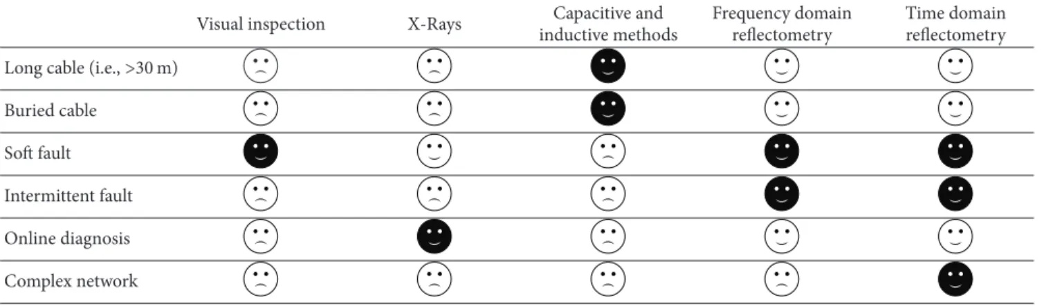
Table 1: Comparison of diagnosis methods: The white smiley face: the method detects the fault. The black smiley face: the method detects the fault under conditions. The white sad face: the method does not detect the fault.
Visual inspection X-Rays inductive methodsCapacitive and Frequency domainreflectometry Time domainreflectometry Long cable (i.e.,>30 m)
Buried cable Soft fault Intermittent fault Online diagnosis Complex network
the energy or information circulation in the damaged cable. They include open circuit and short circuit. On the other hand, soft faults result in a small variation in the characteristic impedance of the cable caused by sheath crack, conductor degradation, and so forth. These faults do not always lead to catastrophic incident as they do not interrupt energy or information circulation, but can generate hot spots and hard faults in over the long term due to mechanical stress, moisture penetration, thermal stress, or even cable aging. An efficient diagnosis system is mandatory to detect and precisely locate the fault(s).
In this context, various methods have been studied such as visual inspection, X-rays, capactive and inductive meth-ods, and reflectometry. While the visual inspection is com-monly used, it is inefficient in complex wired networks. It can detect only 25% of faults present in an aircraft [14] when a large portion of the wired network is hidden by huge struc-tures such as electric panels, components, or other cables. The X-ray inspection requires the use of heavy equipment, direct access to cable, and human intervention for data analysis. Both methods, capacitive and inductive, are efficient in the case of of point-to-point cable diagnosis but remain limited in the case of complex wired networks. In addition, they can be used only if the cable is offline.Table 1summarizes the main advantages and disadvantages of those methods. Among all known diagnosis methods, reflectometry appears to be the most promising one.
Reflectometry includes two main families: Time Domain Reflectometry (TDR) and Frequency Domain Reflectometry (FDR). On the one hand, TDR injects periodically a probe signal and the reflected signal is basically made of multiple copies of this signal delayed in time. For each copy, the delay is the round trip time necessary to reach the discontinuity from the injection point. This signal is called “reflectogram” [15]. So, the knowledge of the propagation velocity and the time delay of each copy permits to locate the corresponding impedance discontinuity. On the other hand, FDR injects a set of sine wave called chirp [16–18]. Then, the analysis of the standing wave permits to give information about the fault location. This analysis becomes difficult to interpret in the case of complex wiring network. For this reason, TDR is more interesting than FDR in complex wiring networks.
3. Orthogonal Multi-Tone Time
Domain Reflecometry
The multicarrier modulation Frequency Division Multiplex-ing (FDM), used by reflectometry MCTDR, divides the bandwidth into several subbands using subcarriers. These subcarriers must be separated by a guard band to avoid interference problems. This leads to nonoptimal use of the available bandwidth. Indeed, up to 50% of the bandwidth is used by the interband intervals [19, 20]. Orthogonal Fre-quency Division Multiplexing (OFDM) is an interesting modulation technique permitting reducing those guard inter-vals and then bandwidth loss. This technique is well known in the fourth generation cellular networks such as Long Term Evolution (LTE) and Worldwide Interoperability for Microwave Access (WiMAX) 802.16, thanks to its capacity to achieve a very high data rate transmission. The idea is to divide the total bandwidth using orthogonal and then over-lapped subcarriers which permits to maximize the spectral efficiency and interference mitigation.
3.1. Modeling and Functional Description of OMTDR Signal.
The OFDM technique consists in dividing the bandwidth𝐵
using𝑁 subcarriers modulated independently by a
Quadra-ture Amplitude Modulation with 𝑀 states (𝑀-QAM). The
𝑀-QAM modulation is a digital modulation that changes the amplitude and the phase of each subcarrier according to binary information to be transmitted on it. In the OMTDR method, the test signal injected down the wiring network is defined as 𝑠𝑘(𝑡) = 𝑁−1 ∑ 𝑛=0𝑆𝑘,𝑛𝑔𝑛(𝑡 − 𝑘𝑇𝑠) , (1)
where𝑛 is the subcarrier number in the considered OFDM
symbol𝑘. Each subcarrier signal 𝑔𝑛(𝑡) is modulated
indepen-dently by the complex valued modulation symbol𝑆𝑘,𝑛and is
expressed as 𝑔𝑛(𝑡) ={{ { 𝑒𝑗2𝜋𝑛Δ𝑓𝑡 if𝑡 ∈ [0, 𝑇 𝑠] 0 if not, (2)
where𝑇𝑠 = 1/Δ𝑓 represents the useful OFDM symbol
dura-tion.Δ𝑓 is the frequency distance between two consecutive
subcarriers. The spectrum of the test signal𝑆𝑘(𝑓) is given by
𝑆𝑘(𝑓) = 𝑇𝑠𝑁−1∑
𝑛=0
𝑆𝑘,𝑛sinc(𝜋𝑇𝑠(𝑓 − 𝑛Δ𝑓)) , (3)
where sinc(𝑥) = sin(𝑥)/𝑥. The injected signal 𝑥𝑘(𝑡) is
obtained by a digital-to-analog conversion (DAC) and cor-responds to the following relation:
𝑥𝑘(𝑡) = +∞∑ 𝑘=−∞ 𝑁−1 ∑ 𝑛=0 𝑆𝑘,𝑛𝑒𝑗2𝜋𝑛Δ𝑓𝑡Π (𝑡 − 𝑘𝑇𝑠) , (4)
whereΠ is the shaping filter and is given as follows: Π (𝑡) ={{
{
1 if 𝑡 ∈ [0, 𝑇𝑠]
0 if not. (5)
The autocorrelation function of the test signal gives an idea about the observed shape at each peak related to the impedance discontinuity. In the OMTDR method, it is expressed as follows: 𝐶𝑠𝑠(𝜏) = 𝑁1 𝑁−1 ∑ 𝑖=0𝑠𝑘,𝑖𝑠 ∗ 𝑘,𝑖−𝜏𝑒−𝑗2𝜋(𝜏𝑛/𝑁), (6)
where𝜏 is the delay and 𝑁 is the number of samples. Indeed, the test signal𝑠𝑘(𝑡) is sampled with the sample interval Δ𝑡 = 1/𝑁Δ𝑓 in numerical applications. Here, the sample of the transmit signal is denoted by𝑠𝑘,𝑖where𝑖 ∈ {0, 1, . . . , 𝑁 − 1} and is expressed as follows:
𝑠𝑘,𝑖=𝑁−1∑
𝑛=0
𝑆𝑘,𝑛𝑒𝑗2𝜋𝑖(𝑛/𝑁). (7)
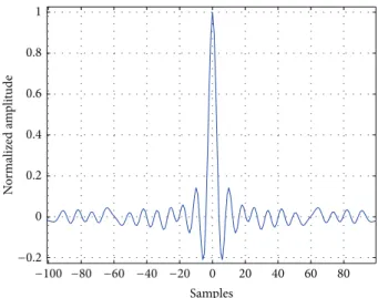
Figure 1shows the autocorrelation function of the OMTDR signal(6). The autocorrelation function is a pulse consisting of a central lobe and side lobes. The presence of side lobes may cause a fault detection problem (false alarm).
Online diagnosis provides the possibility of performing the diagnosis concurrently to the normal operation of the network. However, it imposes serious challenges related to Electro-Magnetic Compatibility (EMC) constraints. When the energy of the test signal should be limited in some frequency bands, the corresponding coefficients𝑆𝑘,𝑛must be canceled as follows:
𝑆𝑘,𝑛= 0 ⇒ 𝑆𝑘(𝑛Δ𝑓) = 0, where 𝑛 ∈ [0, 𝑁 − 1] , 𝑛 ∈ N.
(8) The signal𝑥𝑘(𝑡) given by(4)is injected into the line and is reflected if it meets one or more impedance discontinuities during its propagation.
3.2. Analysis of the Measured Signal Using OMTDR Method. The received signal is represented as the convolution between the test signal and the channel impulse responseℎ𝑘(𝑡) in the
0 20 40 60 80 0 0.2 0.4 0.6 0.8 1 Samples N o rm al iz ed a m p li tude −100 −80 −60 −40 −20 −0.2
Figure 1: Autocorrelation function of the OMTDR signal in the case of 512 samples and 4-QAM modulation.
presence of Additive White Gaussian Noise (AWGN). At the output of the analog-digital converter, the received signal is sampled at the rate1/𝑇𝑠. We can write the following relation:
𝑦𝑘,𝑖= 𝑠𝑘,𝑖∗ ℎ𝑘,𝑖+ 𝑛𝑘,𝑖. (9)
The reflected signal 𝑦
𝑘 = (𝑦𝑘,0, 𝑦𝑘,1, . . . , 𝑦𝑘,𝑁−1) is now
correlated with the test signal𝑠𝑘 = (𝑠𝑘,0, 𝑠𝑘,1, . . . , 𝑠𝑘,𝑁−1) and the obtained signal is given as follows:
𝑟𝑠𝑦𝑘(𝜏) = 𝑁1𝑁−1∑
𝑖=0
𝑠𝑘,𝑖𝑦𝑘,𝑖−𝜏∗ . (10)
In online diagnosis, the modifications of the OMTDR signal spectrum to fulfill the EMC requirements lead to information loss. Indeed, in the frequency domain, the network response is clearly unknown in the canceled frequency bands. To verify this, we take the example of a transmission line of length 100 m with a soft fault at 50 m from the injection point and an open circuit at its end. Here, 50% of the bandwidth is canceled. We note that the loss of information causes the appearance of distortions around the peaks as shown in Figure 2.
The estimation of this missing information requires a spe-cific postprocessing. To do so, we propose here to introduce an averaging step for multiple OFDM symbols as follows:
𝑟𝑠𝑦= 𝐾1𝐾−1∑
𝑘=0
𝑟𝑠𝑦𝑘, (11)
where𝑟𝑠𝑦
𝑘 is the signal obtained from(10)after correlation
between test signal and reflected signal in symbol OFDM𝑘. 𝐾 represents the number of OFDM signals. Note that generated
bits are different from an OFDM symbol to another.Figure 3
shows the obtained reflectogram after averaging 10 measures. As mentioned above, the presence of side lobes (Figure 1) is unsuitable to detect and locate soft faults mainly in complex wiring networks. To improve the analysis of the reflectogram,
50 100 150 200 0 0.1 0.2 0.3 0.4 0.5 Distance (m) N o rm alize d a m p li tude −0.2 −0.1
Figure 2: Obtained reflectogram where samples{0, 1, . . . , 255} are canceled. 0 50 100 150 200 250 0 0.1 0.2 0.3 0.4 0.5 Distance (m) N o rm alized a m p li tude −0.1
Figure 3: Obtained reflectogram after averaging where samples {0, 1, . . . , 255} are canceled.
we propose to introduce a convolution between the measure 𝑟𝑠𝑦and a windowing function𝜔 as follows:
̂𝑟𝑠𝑦̂𝑖= 𝑟𝑠𝑦𝑖∗ 𝑤𝑖, (12)
where𝑖 is the sample of the measure 𝑖 ∈ {0, 1, . . . , 𝑁−1} and 𝑖 is the sample of the windowing function𝑖∈ {0, 1, . . . , 𝑁−1}.
𝑁 and 𝑁represent the number of samples of the measure
and the windowing function, respectively. The number of
samples of the convoluted signal is noted ̂𝑁 where ̂𝑁 =
𝑁+𝑁−1. The Dolph-Chebyshev window seems to be the best
window to achieve a good compromise between the width of the central lobe at mid-height and the amplitude of the side lobes [21,22].Figure 4shows the obtained reflectogram after
convolution with a Dolph-Chebyshev window where𝑁 =
20.Figure 5shows the principle of OMTDR reflectometry for online diagnosis. 50 100 150 200 250 0 0.1 0.2 0.3 0.4 0.5 Distance (m) N o rm alized a m p li tude −0.1
Figure 4: Obtained reflectogram after postprocessing where sam-ples{0, 1, . . . , 255} are canceled.
4. Fault Location Ambiguity Problems in
Complex Branched Networks
In complex wiring network, using a single sensor is no longer possible to cover the whole network. This may be explained by the signal attenuation due to the distance and multiple junc-tions. Although the distance between the injection point and the fault may be determined, the identification of the defected
branch remains ambiguous. To illustrate this, Figure 7
shows the computed reflectogram for the branched network ofFigure 6with an open circuit fault at 25 m from the injec-tion point. Only one reflectometer is placed at the extremity
of𝐿1to diagnose the whole network. The reflectometer and
the network are considered unmatched, explaining the first positive peak on the reflectogram. The ends of lines are also unmatched. Here, the detected fault on𝐿3cannot be distin-guished from the same fault on𝐿2. In this case, it is possible
to add another reflectometer at the end of 𝐿2 using
dis-tributed diagnosis. The ambiguity disappears thanks to this new sensor but would recur upon the occurence of a new fault on𝐿4. So, another reflectometer should be added to overcome this ambiguity. Then, distributed reflecometry is a suitable method to overcome ambiguity problems. However, several challenges are imposed related to interference mitigation when all sensors use the network simultaneously. In the context of multicarrier method, we propose to use Frequency Division Multiple Access (FDMA) method as shown later.
5. A New Subcarrier Allocation Method for
Interference Mitigation
The use of OMTDR signal made of orthogonal subcarriers allows the avoidance of an interference by allocating a different set of available subcarriers to each sensor. The con-ventional method is to allocate to each sensor a set of adjacent
subcarriers.Figure 8shows a spectrum of OMTDR method
whose subcarriers are divided into three sensors 𝑆1, 𝑆2, and𝑆3. Taking the subcarriers in ascending values of their
Data generation
M-QAM
modulation S/P IFFT P/S DAC
ADC Correlation
Reflectogram
analysis Convolution Averaging Windowing function Sk Sk,0 Sk,1 Sk,n Sk,N−1 .. . .. . .. . .. . xk(t) Wired networks xk(t) ∗ hk(t) + nk(t) yk(t) y k rsy rsy ̂rsy 𝜔 sk sk,0 sk,1 sk,n sk,N−1
Figure 5: Principle of OMTDR reflectometry for online diagnosis.
Diagnosis system Fault Ambiguous fault L1(20 m) L2(15 m) L3(15 m) L4(5 m) L5(20 m)
Figure 6: Fault location ambiguity in a branched network.
0 10 20 30 40 50 60 70 80 90 0 0.1 0.2 0.3 0.4 0.5 Am p li tude (V) Distance (m) Faulty network Junction Fault End of line L2 −0.5 −0.4 −0.3 −0.2 −0.1
Figure 7: Reflectogram using TDR method.
central frequencies, a first group (low frequencies) of adjacent
subcarriers (3 subcarriers in the example in Figure 8) is
allocated to 𝑆1. A second group (medium frequencies) of
adjacent subcarriers is assigned to𝑆2. Finally, a third group
Sensor S1
Sensor S2
Sensor S3
Low frequencies Medium frequencies High frequencies
Am p li tude Frequency · · · ·
Figure 8: Example of adjacent subcarriers allocation.
(high frequencies) of adjacent subcarriers is allocated to𝑆3. Although adjacent subcarriers allocation method permits to avoid interference, it has drawbacks. Indeed, in the con-figuration of Figure 8, 𝑆1 uses subcarriers located substan-tially at low frequencies,𝑆2 uses subcarriers located in the
medium frequencies, and𝑆3 uses subcarriers located in the
higher frequencies. This difference in spectrum causes unfor-tunately a difference in perspective of the network seen by each sensor. Therefore, the quality of the 3 obtained reflec-tograms is different in this case. In fact, propagation phenom-ena (attenuation and dispersion) depend extremely on the signal frequency. So, the attenuation and dispersion is more important in high frequencies than in low frequencies. For all these reasons, adjacent subcarriers allocation is not efficient in the reflectometry-based wire diagnosis. Thus, we propose a distributed subcarriers allocation method as shown in Figure 9. In this case, each sensor uses subcarriers in regularly distributed frequencies and, thus, all sensors use signals operating at similar frequencies.
In the example inFigure 9, the subcarriers are alternately allocated to one of three reflectometers 𝑆1, 𝑆2, and 𝑆3. Proceeding in this way, we ensure that each sensor𝑆1, 𝑆2, and𝑆3 will generate a multicarrier signal using frequencies uniformly distributed in the useful band. All generated sig-nals have then a close spectral profile which ensures obtaining homogeneous reflectograms. Three sensors𝑆1,𝑆2, and𝑆3are implemented in the network shown inFigure 6.𝑆1,𝑆2, and𝑆3 are related, respectively, to branches𝐿1,𝐿2, and𝐿4. Here, the
Sensor S1
Sensor S2
Low frequencies Medium frequencies High frequencies
Am p li tude Frequency Sensor S3 · · · ·
Figure 9: Example of distributed subcarriers allocation.
0
Junction
Round-trip on the fault −0.6 0.2 0.4 0.6 0.8 Am p li tude 10 15 20 25 30 35 40 Distance (m) Adjacent allocation Distributed allocation −0.4 −0.2 Fault on L3 Figure 10: Reflectogram of𝑆1.
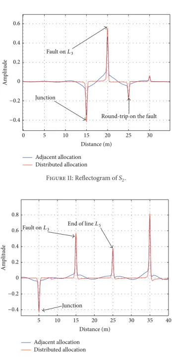
sensors and the branches are considered matched. The branch 𝐿5is affected by an open circuit at its end. Figures10,11, and12 show the obtained reflectograms by sensors𝑆1,𝑆2, and𝑆3in two cases: allocation of subcarriers is performed as described inFigure 8(adjacent allocation) and allocation of subcarriers is performed as described inFigure 9(distributed allocation). We remark that the distributed allocation method permits enhancing the quality of the reflectograms compared to the adjacent allocation method particularly in the case of sensors 𝑆2and𝑆3using medium or high frequencies.
After interference mitigation in distributed reflectometry, we propose now to integrate communication between sensors via the transmitted part of the test signal which has never been done with conventional methods [9,10]. For this reason, the test signal must be capable of carrying information which is possible thanks to the OMTDR method [11]. The fusion of all this information, based on master/slave protocol, provides unambiguous location of the fault in complex wired networks as shown as follows.
6. Data Fusion for Wire Fault Location
In this section, we propose to integrate communication between sensors to enable data fusion in the context of distributed diagnosis. For this reason, we propose to use
0
Junction
Round-trip on the fault 0 0.2 0.4 0.6 Am p li tude 5 10 15 20 25 30 Distance (m) Adjacent allocation Distributed allocation −0.4 −0.2 Fault on L3 Figure 11: Reflectogram of𝑆2. 0 0.2 0.4 0.6 0.8 Am p li tude 5 10 15 20 25 30 35 40 Distance (m) Junction Adjacent allocation Distributed allocation −0.4 −0.2
Fault on L3 End of line L5
Figure 12: Reflectogram of𝑆3.
not only the reflected part of the diagnosis signal, but also the transmitted part. A signal carrying information is then used as test signal to enable reflectometry measurement and communication through the OMTDR technique. To do so, let us begin with the structure of the test signal.
6.1. Frame Description. As the test signal is carrying informa-tion, the data is formatted into frames themselves subdivided into 9 fields. The frame is delimited by a Start Of Frame (SOF) (8 bits) and an End of Frame (EOF) (8 bits) field. Each sensor is identified in the network by an ID (16 bits). Then, the field CMD (8 bits) reveals the nature of the frame (data or request). The field DLC gives the length of the transmitted data that may vary between 21–53 bytes. Cyclic Redundancy Check
SOF 8 bits CMD 8 bits DLC 8 bits EOF 8 bits Data 22–53 bytes ID dest 16 bits ID source 16 bits CRC 16 bits ACK 2 bits
Figure 13: A frame structure.
Transmission line (0 junctions) Y shaped network (1 junction) 2 junctions 3 junctions 4 junctions 5 junctions Transmitter Receiver Junctions Network topology
Figure 14: Evolution of the topology of the network.
(CRC) is used for error detection as shown byFigure 13and
ACK to acknowledge the good receipt of the message. After having described the frame structure, we propose now to classify the distributed sensor into two groups: master and slave.
6.2. Classification of Sensors. In master/slave protocol, the choice of the master is crucial to ensure the efficiency of the proposed diagnosis strategy. To do so, we propose to assign a weight of eligibility to each sensor for sensor classification. In fact, the reflectogram’s quality depends strongly on the network topology in terms of distance and number of junctions [1]. The same remark holds for the communication quality. We propose now to study the impact of network topology on communication quality. We focus only on the number of junctions in the network. Recall that a junction causes the reflection of a part of the energy of the transmitted signal.Figure 14shows the different topologies considered in order to calculate the BER. For this, the distance between the transmitter and the receiver is set to 10 m and the SNR is
10 dB.Figure 15shows the evolution of the BER versus the
number of junctions in the network. It may be noted that the BER depends on the complexity of the network topology in terms of junctions number. Indeed, the increase of the number of junctions causes the increase of the attenuation of the signal during its propagation.
0 1 2 3 4 5 0.1 0.2 0.3 0.4 0.5 0.6 0.7 Number of junctions BER (%) 0 junctions 1 junction 2 junctions 3 junctions 4 junctions 5 junctions
Figure 15: Evolution of bit error rate in terms of junctions number.
Based on these findings, the weight of eligibility may be calculated by the following parameters.
(i) The sum of distances𝐷𝑆𝑖 = ∑𝑆𝑗∈𝑉
𝑆𝑖distance(𝑆𝑖, 𝑆𝑗)
between sensor𝑆𝑖 and the other sensors𝑆𝑗, 𝑖 ̸= 𝑗 where 𝑉𝑆𝑖 is the set of sensors in the network. The minimization of this value reduces the propagation attenuation and hence the bit error rate.
(ii) The number of junctions𝐽𝑆𝑖 = ∑𝑆
𝑗∈𝑉𝑆𝑖junction(𝑆𝑖, 𝑆𝑗)
between sensor𝑆𝑖and the other sensors𝑆𝑗,𝑖 ̸= 𝑗. The minimization of this value reduces the bit error rate due to multiple reflections as shown byFigure 15. The weight of eligibility for sensor𝑆𝑖is given by
𝑤𝑆𝑖 = 𝐷𝑆𝑖× 𝐽𝑆𝑖. (13)
In fact, the minimization of the weight of eligibility reduces firstly the bit error rate and increases the diagnosis accuracy since it minimizes the attenuation of the test signal. Then, the sensor with the lowest weight of eligibility is designated as the master while other sensors are consid-ered as slaves. Besides network diagnosis (signal injection, received signal processing, fault detection, etc.), the master must ensure the management of its slaves (synchronization, resource allocation, routing table, etc.), the information collection, data analysis, and decision making. For their part, slaves must do their diagnosis, identify the fault position, and send it to their master.
Construct the reflectogram of the new measure Yes No No No Yes Start End extrema of reflectogram
𝜍curr← extract local
𝛼curr(i) < T? ecurr(i) ∈ 𝜍ref? i = Ncurr?
i = i + 1
𝜍ref← 𝜍ref+ {ecurr(i)} 𝜍d← 𝜍d+ {ecurr(i)}
𝜍ref= {ecurr(1), . . . ecurr(i), . . . , ecurr(Ne)}
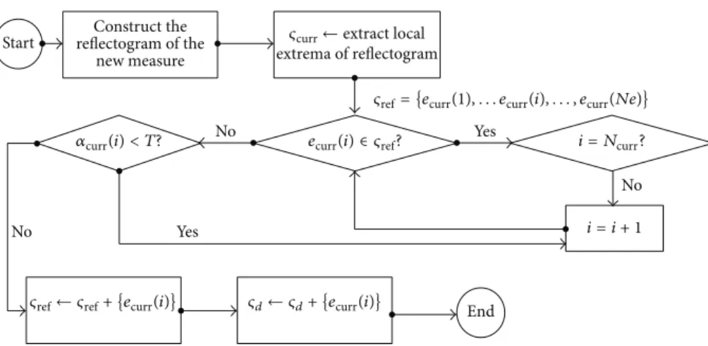
Figure 16: Algorithm for detecting and locating faults in a single measurement.
6.3. Automation of Fault Detection and Location. In this section, we propose to develop an algorithm to automate the detection and location of a fault. We propose firstly to gen-erate a reference measurement obtained when the network is healthy. We propose to save in sensor memory only the position of the local extrema of the corresponding reflec-togram to avoid the saturation of the embedded memory. The number of extrema in the reference is noted𝑁ref. The set of
extrema is𝜍ref= {𝑒ref(1), 𝑒ref(2), . . . , 𝑒ref(𝑁ref)}. We
character-ize each extremum by its position and amplitude as follows: (𝑝ref(𝑖), 𝑎ref(𝑖)) where 𝑖 ∈ {1, 2, . . . , 𝑁ref}.Figure 16describes
the proposed algorithm for detecting and locating automat-ically a possible fault. After the construction of the reflec-togram, we extract local extrema noted𝑒curr(𝑝curr(𝑖), 𝑎curr(𝑖)).
Then, we compare it in terms of position with those stored in memory (reference). This indicates whether there has been an evolution of the state of the network or not. We note𝜍curr =
{𝑒curr(1), 𝑒curr(2), . . . , 𝑒curr(𝑁curr)}, where 𝑁curris the number
of extrema in the current measure. If there is no change, we must ensure that all local extrema are treated. Otherwise,
we should treat the following extremum where𝑖 ← 𝑖 + 1.
However, if the detected extremum does not belong to the reference set𝜍ref, we must determine whether the amplitude
of the extremum value is greater than a threshold noted𝑇 to avoid considering noise as a fault. In the presence of AWGN noise, the threshold is expressed as follows:
𝑇 = 2𝑁𝜎2, (14)
where𝑁 represents the number of samples and 𝜎 the AWGN
variance.
The algorithm described above allows automatic detec-tion and locadetec-tion of a fault in a single reflectometry measure-ment. Indeed, saving only local extrema permits to optimize both processing time and memory capacity. Thereafter, the position of the detected fault is encapsulated in the field data of the frame to be sent to the master if the actual sensor is a slave.
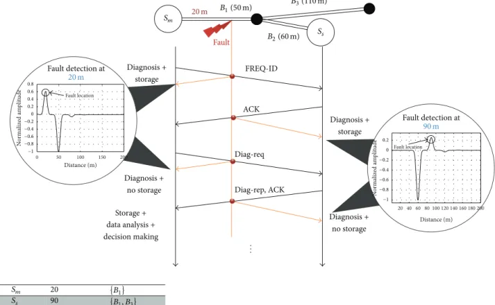
6.4. Description of the Communication Protocol. The
mas-ter noted 𝑆𝑚 sends a data message for initialization with
CMD = “FREQ-ID” and the data field contains the set of subcarriers allocated to the slave𝑆𝑠as seen inSection 5and shown on the upper part ofFigure 17.
Considering a soft fault withΔ𝑍𝑐 = 20% on the branch
𝐵1, a part of energy of the message sent by𝑆𝑚is reflected back.
The master 𝑆𝑚 constructs the corresponding reflectogram
and detects the presence of the soft fault at 20 m from𝑆𝑚
based on the algorithm shown in Figure 16. The soft fault
position is stored in the memory of sensor𝑆𝑚. After receiving the initializing message of its master𝑆𝑚, the salve𝑆𝑠injects an OMTDR signal which contains an acknowledge message
to 𝑆𝑚 where CMD = “ACK” and the filed ACK = “01”. In
order to avoid that the data field remains empty (diagnosis precision degradation), a zero padding with at least 21 bytes is done. Here, a part of energy of the message is reflected back and the slave defines the fault position at 90 m based on its reflectogram. This position is also stored in its memory. Note that the processing of the measurement is done locally. For this, the slave must have a good memory and processing capacity.
When master 𝑆𝑚 receives the acknowledgment of its
salve, a new request message where CMD = “Diag-Req” is sent to𝑆𝑠for information providing. The sensor must, every time, analyze the new reflectogram and compare it with that obtained at the previous time to check if the fault persists, if it has evolved (amplitude variation, increasing the length, etc.) or even if there is another fault that appeared in the meantime, and so forth. The slave𝑆𝑠sends a data message where CMD = “Diag-Req” containing the information about the fault posi-tion. At the reception, the master𝑆𝑚 extracts the data sent by its slave and stores it in its memory. After receiving data sent by all its slaves, the master analyzes this data and makes the decision about the fault location in the network. In this
example, the fault is located on branch 𝐵1 as shown by
Figure 17.
The data fusion, based on master/slave protocol, provides unambiguous location of the fault in complex wired network. Moreover, it may provide information about the state (i.e., out of service) of the sensors in the network. We propose to verify the efficiency of data fusion strategy in a CAN bus system.
20 90 FREQ-ID ACK Diag-req Diag-rep, ACK Diagnosis + no storage Storage + data analysis + decision making Fault Diagnosis + storage Diagnosis + storage Diagnosis + no storage Fault location Fault location 0 50 100 150 200 Distance (m) Distance (m) N o rm al iz ed a m p li tude 20 40 60 80 100 120 140 160 180 200 −1 −0.8 −0.6 −0.4 −0.2 0 0.2 N o rm al iz ed a m p li tude −1 −0.8 −0.6 −0.4 −0.2 0 0.2 0.4 0.6 0.8 Fault detection at 20 m 20 m Fault detection at 90 m .. . Sm Sm Ss Ss B1(50 m) B2(60 m) B3(110 m) {B1, B3} {B1}
Figure 17: Scenario of the communication protocol.
CAN CAN CAN
CAN CAN CAN B4 B5 B6 B7 B1 B2 B3 120 Ω 120 Ω B4 B2 B1 B3 B5 B6 S1 S2 S3 S4 S5 S6
Figure 18: CAN bus system.
6.5. Validation of the Strategy in a CAN Bus System. In this section, we consider the CAN bus system described in Figure 18. The network consists of six sensors 𝑆𝑖, 𝑖 ∈ {1, 2, . . . , 6} with the same characteristics (homogeneous network). These sensors are considered matched with the
network cables where𝑍𝑐 = 120 Ω. The bus is divided into
multiple portions noted from 𝐵1 to 𝐵7 with lengths 5 m,
8 m, 13 m, 26 m, 8 m, 18 m, and 22 m, respectively. The cables that connect the electronic functions to ensure access to the network are denoted, respectively,𝐵1to𝐵6with length of 5 m. We consider the presence of a soft fault with length of 0.5 m
on branch𝐵3and variation of the impedance related to the
characteristic impedance Δ𝑍𝑐 = 20%. Here, the master
manages 5 slaves.
Table 2: Weight of eligibility of each sensor.
𝑖 = 1 𝑖 = 2 𝑖 = 3 𝑖 = 4 𝑖 = 5 𝑖 = 6
𝐷𝑆𝑖 254 222 196 196 212 284
𝐽𝑆𝑖 20 16 14 14 16 20
𝑤𝑆𝑖 5080 3552 2744 2744 3392 5680
Firstly, we calculate the weight of each reflectometer using (13).Table 2shows the weight of eligibility of each sensor.
It may be noted that both sensors 𝑆3 and 𝑆4 have the
lowest weight. If we were in a heterogeneous case, we could differentiate between the two sensors by another metric such as reliability, computing, or memory capacity and so forth. However, we have assumed a homogeneous case in this paper. As a result, we can choose either sensor𝑆3or𝑆4. In this case, we will consider the sensor𝑆4as the master. Using the strategy described above, each slave must detect and locate the soft fault and send it to its master𝑆4. Figures19and20show reflectograms obtained by salves𝑆5and𝑆6, respectively. The
positions of the fault are then sent to master 𝑆4. After
receiving all data of its slaves, the master makes the decision on the location of the fault in the whole network.
Table 3shows the available data at master𝑆4. Given that the network topology is already known by the master, it is able to locate the fault on branch𝐵3. It is noted that the amount of information depends heavily on the complexity
Table 3: Fault location on branch𝐵3.
Sensor Distance of the fault
from sensor Ambiguous branches
𝑆1 18 {𝐵2, 𝐵3} 𝑆2 10 {𝐵2, 𝐵3} 𝑆3 39 {𝐵4, 𝐵3} 𝑆4 55 {𝐵7, 𝐵3} 𝑆5 47 {𝐵3} 𝑆6 65 {𝐵3} 10 20 30 40 50 60 70 80 Distance (m) N o rm alize d a m p li tude Junction 1 Junction 2 Junction 3 Junction 4 Soft fault X: 47 Y: −0.06886 −1 −0.8 −0.6 −0.4 −0.2 0 0.2
Figure 19: Reflectogram of𝑆5: fault location at 47 m.
10 20 30 40 50 60 70 Distance (m) N o ra malize d a m p li tude Junction 1 Junction 2 Junction 3 Soft fault X: 65 Y: −0.01441 −0.45 −0.4 −0.35 −0.3 −0.25 −0.2 −0.15 −0.1 −0.05 0
Figure 20: Reflectogram of𝑆6: fault location at 65 m.
of the network topology and the number of sensors. This directly affects the decision-making time.
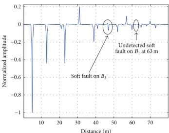
Sensor fusion is an innovative solution in the field of reflectometry. This can be achieved through the use of a signal carrying information thanks to the OMTDR method. The sensor fusion allows the centralization of information and facilitates decision-making about the fault location in the whole network. Soft fault on B3 Undetected soft fault on B1at 63 m 10 20 30 40 50 60 70 Distance (m) N o rm alize d a m p li tude −1 −0.8 −0.6 −0.4 −0.2 0 0.2
Figure 21: Reflectogram of𝑆5: undetected fault at 63 m.
0 80 90
Soft fault on B3 X: 65
Y: −0.03094
Undetected soft fault on B1at 81 m
10 20 30 40 50 60 70 Distance (m) N o rm alize d a m p li tude −1 −0.9 −0.8 −0.7 −0.6 −0.5 −0.4 −0.3 −0.2 −0.1 0
Figure 22: Reflectogram of𝑆6: undetected fault at 81 m.
We consider now the presence of a new soft fault on
branch 𝐵1 with a relative variation of the characteristic
impedanceΔ𝑍𝑐= 20%. Figures21and22show reflectograms
of slaves𝑆5and𝑆6, respectively. Note that the soft fault can not be detected either by sensor𝑆5or by sensor𝑆6because of signal attenuation after 5 or 6 junctions. Thus, both sensors always send information about the fault previously detected on branch𝐵3. In this case, there is a fault location ambiguity relative to the master𝑆4as shown inTable 4.
In the context of complex wiring networks, data fusion strategies suffer from signal propagation phenomena (atten-uation and dispersion) which affect the diagnosis reliability for reflectometry measurement and data credibility for com-munication. In addition, the increase of complexity of the network topology comes with the increase of the amount of information, the time of information analysis and decision making. When a hard fault (open circuit or short circuit) appears, the master may be unreachable. As a solution, we propose a sensor clustering strategy.
Table 4: Ambiguity of fault location.
Sensor Distance of the fault
from sensor Ambiguous branches
𝑅1 8 {𝐵1, 𝐵2} 𝑅2 16 {𝐵3, 𝐵1, 𝐵1} 𝑅3 29 {𝐵4, 𝐵1, 𝐵1} 𝑅4 55 {𝐵1, 𝐵1} 𝑅5 47 {𝐵3} 𝑅6 65 {𝐵3}
7. Sensors Clustering in Complex Networks
In the case of complex topology, the network is divided into subnetworks with simpler topologies. We are talking here about sensor clustering. It consists in the network partition into clusters of one or more specific metric(s). Each cluster is controlled by a master to manage its slaves (synchronization, resource allocation, routing table, etc.), collect information, and make a decision on the fault location. Each slave is responsible for communication within the cluster but must also maintain information corresponding to neighboring clusters (e.g., the identifier of the master of a neighboring cluster, the path to join, etc.).
In fact, the communication and diagnosis qualities depend strongly on the distance and number of junctions. For this reason, we consider these two parameters in the cluster-ing strategy. To do so, we consider that the maximum number of junctions between two sensors of the same cluster must be less or equal to 3. First of all (step 1), for each sensor, one or many set(s) of possible sensors satisfying the above condition is/are defined. In step 2, we propose to compute for each sensor the sum of distances between sensors of the same set. The list that presents the lowest distance is selected for each sensor in step 3. Finally, clusters may be defined based on the obtained sets.
To demonstrate the interest of sensor clustering in a complex network, we consider the CAN bus system shown onFigure 18. In order to define sensor clusters, we define for each sensor the set of sensors where the number of junctions is equal to 3. Then, we use the sum of distances for each set in order to choose the best set of each sensor. Based on the sum of distances in each set, it is possible now to select the best set
of sensors for each sensor.Table 5summarizes the strategy
previously described.
By considering the intersection between the different sets, we are able to divide the network into two clusters noted𝐶1 and𝐶2.Table 6shows the sensors and diagnosed branches assigned to each reflectometer. It may be noted that a branch can be covered by sensors belonging to different clusters.
After sensors clustering, we propose now to identify the
master for each cluster. Here, we consider only cluster𝐶1
where𝑆2is considered as master and𝑆1and𝑆3are slaves as shown byTable 7.
Table 8 shows the diagnosed branches of cluster 𝐶1. It should be noted that the signal propagation is limited by acquisition windows (or observation).
Soft fault B1+ B2 B1 B1+ B2+ B2 B1+ 3 ∗ B2+ B2 0 5 10 15 20 25 Distance (m) Am p li tude 10 20 30 40 50 60 0 0.5 1 Distance (m) Am p li tude −1 −0.5 0
Fault location at 21 m from S1
Transmission function from S1to S2
Figure 23: Fault location at 21 m from𝑆1and transmission of the fault position to𝑆2. 0 5 10 15 20 25 30 Distance (m) Am p li tude 0 10 20 30 40 50 60 0 0.5 1 Distance (m) Am p li tude Soft fault Soft fault B3+ B3 B3 B3+ B3+ B2 B3+ B3+ B2 B3+ 3 ∗ B3+ B2 −1 −0.5 0
Fault location at 10 m from S3
Transmission function from S3to S2
Figure 24: Fault location at 10 m from𝑆3and transmission of the fault position to𝑆2.
Figures23and24(top) show reflectograms obtained by𝑆1 and𝑆3, respectively. The soft fault is detected at 21 m and 10 m from𝑆1and𝑆3, respectively. These positions are then sent to master𝑆2as shown by Figures23and24(bottom). The first peak at 18 m corresponds to the direct path between𝑆1and𝑆2 (sum of lengths of branches𝑙𝐵
2 = 5 m, 𝑙𝐵2 = 8 m, 𝑙𝐵1 = 5 m).
The other peaks correspond to the multipath signal following multiple reflections. Same observation for sensor𝑆3at 23 m is found.
Based on its own information and that sent by its slaves 𝑆1and𝑆3, master𝑆2locates the fault on branch𝐵3as shown inTable 9.
We consider now the presence of a second soft fault on𝐵1. Figures25and26show reflectograms obtained by𝑆1and𝑆3. The fault is detected at 8 m and 29 m of𝑆1and𝑆3, respectively.
Table 5: Sensor clustering in CAN bus using the proposed strategy.
Sensor Step 1: possible set(s) Step 2: sum of distances Step 3: selected set
𝑆1 {𝑆2, 𝑆3} 49 m {𝑆2, 𝑆3} 𝑆2 {𝑆{𝑆1, 𝑆3} 41 m {𝑆1, 𝑆3} 3, 𝑆4} 72 m 𝑆3 {𝑆4, 𝑆5} 80 m {𝑆1, 𝑆2} 54 m {𝑆1, 𝑆2} {𝑆2, 𝑆4} 59 m 𝑆4 {𝑆5, 𝑆6} 54 m {𝑆5, 𝑆6} {𝑆2, 𝑆3} 85 m {𝑆3, 𝑆5} {𝑆3, 𝑆5} 54 m 𝑆5 {𝑆{𝑆4, 𝑆6} 46 m {𝑆4, 𝑆6} 3, 𝑆4} 62 m 𝑆6 {𝑆4, 𝑆5} 64 m {𝑆4, 𝑆5}
Table 6: Allocation of sensors and branches to clusters.
Cluster Associated sensors Traveled branches
𝐶1 𝑆1,𝑆2,𝑆3 {𝐵1, 𝐵1, 𝐵2, 𝐵2, 𝐵3, 𝐵3, 𝐵4}
𝐶2 𝑆4,𝑆5,𝑆6 {𝐵4, 𝐵4, 𝐵5, 𝐵5, 𝐵6, 𝐵6, 𝐵7} Table 7: Calculation of the weight of eligibility of sensors of cluster 𝐶1.
𝑖 = 1 𝑖 = 2 𝑖 = 3
𝐷𝑆𝑖 49 41 54
𝐽𝑆𝑖 5 4 5
𝑤𝑆𝑖 254 146 270
Table 8: Diagnosed branches by𝑆1,𝑆2, and𝑆3.
Sensor Diagnosed branches Acquisition window
𝑆1 𝐵1, 𝐵1, 𝐵2, 𝐵2, 𝐵3 26 m
𝑆2 𝐵
2, 𝐵2, 𝐵3, 𝐵1, 𝐵1 18 m
𝑆3 𝐵
3, 𝐵3, 𝐵4, 𝐵2, 𝐵2, 𝐵1, 𝐵1 31 m
Table 9:𝑆2: Soft fault location on𝐵3.
Sensor Distance of the fault from sensor Ambiguous branches
𝑆1 21 {𝐵3, 𝐵2}
𝑆2 12 {𝐵3, 𝐵2}
𝑆3 10 {𝐵3, 𝐵4}
Table 10:𝑆2: Soft fault location on𝐵1.
Sensor Distance of the Fault from Sensor Ambiguous Branches
𝑆1 8 {𝐵1, 𝐵2}
𝑆2 16 {𝐵3, 𝐵2, 𝐵1, 𝐵1}
𝑆3 29 {𝐵4, 𝐵1, 𝐵1}
Based on its own information and that sent by its slaves𝑆1 and𝑆3, the master𝑆2locates the fault on branch𝐵1as shown inTable 10. Let us recall that the location of the second fault on branch𝐵1was not possible without sensor clustering.
0 5 10 15 20 25 30 0 0.2 0.4 Distance (m) Am p li tude Soft fault on B3 Soft fault on B1 −1 −0.8 −0.6 −0.4 −0.2
Figure 25: Fault location at 8 m from𝑆1.
The sensor clustering strategy reduces the amount of information to analyze and consequently and decreases the processing and decision-making time. The clustering also reduces the communication quality degradation due to the increased bit error rate in the case of complex wired network.
8. Experimental Results
In this section, we propose to evaluate the performance
of the clustering strategy using real networks. Figure 27
shows the considered system design. The OFDM signals are calculated offline in MATLAB and downloaded to a Tektronix AWG7122C Arbitrary Wave Generator. We should notice that real OFDM signals are obtained by constraining the input frequency symbols to the IFFT block to have an Hermitian symmetry [23]. The reflected signals and the cor-responding reflectograms are obtained using an oscilloscope (LeCroy Waverunner 204MXi-A 2 GHz). The reflectogram is constructed using correlation function between the injected and reflected signals.
Soft fault on B3 Soft fault on B1 5 10 15 20 25 30 0 0.2 Distance (m) Am p li tude −1 −0.8 −0.6 −0.4 −0.2
Figure 26: Fault location at 29 m from𝑆3.
Oscilloscope Arbitrary wave generator Network to diagnose Reflected signal Injected signal Reflectogram
Figure 27: Experimentation system design: arbitrary wave genera-tor (Tektronix AWG7122C) and oscilloscope (LeCroy Waverunner 204MXi-A 2 GHz).
In order to evaluate the performance of clustering strat-egy, we propose to consider the complex network topology
described in Figure 18. It consists in multiple SMA cables
with characteristic impedance 50Ω noted from 𝐵1 to 𝐵7
with lengths 1 m, 1.9 m, 1 m, 1 m, 0.6 m, 0.5 m, and 0.5 m, respectively. The SMA cables that ensure access to the network are denoted, respectively,𝐵1to𝐵6with lengths 1 m, 0.5 m, 1.9 m, 2.5 m, 1 m, and 1.9 m. The ends of lines are
matched using 50Ω resistors. A soft fault with length of
1 cm is created on branch 𝐵3. In this study, we consider
firstly the network diagnosis without clustering strategy and secondly the network diagnosis with clustering strategy. Here, we consider the same masters and slaves defined previously for the two cases.
8.1. Network Diagnosis without Clustering Strategy. In this case, we consider that the reflectometers𝑆5and𝑆6are slaves as
demonstrated inSection 6.5.Figure 28shows the diagnosed
network by𝑆5. Soft fault B5(1 m) B 3(1.9 m) B3(1 m) B4(1 m) B5(0.6 m) B4(2.5 m) B6(0.5 m) B7(0.5 m) B6 (1.9 m)
Figure 28: Diagnosed network by reflectometer𝑆5.
0 0.2 0.4 0.6 0.8 1 1.2 Am p li tude (V) Faulty network Healthy network 0 1 2 3 4 5 Distance (m) −0.2 Junction 1 (B5) Junction 2 (B5+ B6) Junction 2 (B5+ B5) Junction 3 (B5+ B5+ B4)
Figure 29: Soft fault location by𝑆5at 3.05 m.
Figure 29 shows the reflectogram obtained by 𝑆5. The negative peaks correspond to the junctions located at 1 m, 1.5 m, 1.6 m, and 2.5 m from the injection point. The soft fault is detected at 3.05 m from reflectometer𝑆5as shown on Figure 30. This information is sent by the slave𝑆5to its master 𝑆4.
Figure 31 shows the reflectogram obtained by 𝑆6. The negative peaks correspond to the junctions located at 1.9 m, 2.4 m, 3 m, and 4 m from the injection point. The slave𝑆6is unable to detect the presence of the soft fault due to the signal attenuation (after 4 junctions) as shown onFigure 32. So, it sends to its master𝑆4wrong information about the soft fault location which causes false alarms.
In the case of complex wiring network (Figure 28), reflec-tometry method suffers from signal propagation phenom-ena (attenuation and dispersion) which affect the diagnosis reliability. As a solution, we propose to consider a sensor clustering strategy.
8.2. Network Diagnosis with Clustering Strategy. In clustering strategy, the complex network is divided into subnetworks with simpler topologies where each subnetwork is a cluster.
0 1 2 3 4 5 Distance (m) 0 1 2 3 4 5 6 7 8 9
Soft fault location
X: 3.053 Y: 0.0008029 Am p li tude (V 2) ×10−4
Figure 30: Slave𝑆5: the difference between the two reflectograms in faulty and healthy cases.
Junction 1 (B6) Junction 2 (B6+ B6) Junction 3 (B6+ B6+ B5) 0 0.2 0.4 0.6 0.8 1 1.2 Am p li tude (V) Faulty network Healthy network 0 1 2 3 4 5 Distance (m) −0.2 Figure 31: Reflectogram of𝑆6. 2.5 3 3.5 4 4.5 5 5.5 6 10 Distance (m) ×10−5 0 2 4 6 8 Am p li tude (V 2)
Figure 32: Impossibility of soft fault location by𝑆6.
T-junction
Soft fault
B3(1.9 m)
B3(1 m)
B4(1 m)
Figure 33: Diagnosed network by reflectometer𝑆3.
0 0.5 1 1.5 2 2.5 3 Distance (m) Soft fault Junction 1 (B3) 0 0.2 0.4 0.6 0.8 1 1.2 Am p li tude (V) Faulty network Healthy network −0.2
Figure 34: Reflectogram of𝑆3: soft fault location at 2.44 m.
Here, we consider the cluster 𝐶1 consisting in two slaves
𝑆1 and 𝑆3 and a master 𝑆2. Figure 33 shows the diagnosed
network by 𝑆3. We should notice that a simpler network
is considered only for measurements. However, this simpli-fication is obtained using time windowing in operational application.
Figure 34shows the reflectogram obtained by the slave𝑆3. The first negative peak corresponds to the junction at 1.9 m. Then, the soft fault is detected at 2.44 m from reflectometer 𝑆3as shown onFigure 35.
Figure 36shows the reflectogram obtained by the slave𝑆1. The first negative peak corresponds to the junction at 1 m and the second one corresponds to the second junction at 2.9 m. Then, the soft fault is detected at 3.27 m from reflectometer𝑆3 as shown onFigure 37.
Figure 38shows the reflectogram obtained by the master 𝑆2. The first negative peak corresponds to the junction at 0.5 m. The soft fault is detected at 1.05 m from reflectometer 𝑆2as shown onFigure 39.
Based on its own information and that sent by its slaves𝑆1 and𝑆3, the master𝑆2locates the fault on branch𝐵3as shown inTable 11. Let us recall that the location of the fault on branch 𝐵3was not possible without sensor clustering strategy.
0 2 4 6 8 10 0 2 4 6 8 10 12 Distance (m)
Soft fault location
X: 2.441 Y: 0.00126 Am p li tude (V 2) ×10−4
Figure 35: Slave𝑆3: the difference between the two reflectograms in faulty and healthy cases.
Soft fault Junction 1 (B1) Junction 2 (B1+ B2) 0 0.2 0.4 0.6 0.8 1 1.2 Am p li tude (V) Faulty network Healthy network 0 1 2 3 4 5 Distance (m) −0.2
Figure 36: Reflectogram of𝑆1: soft fault location at 3.27 m.
0 0.5 1 1.5 2 2.5 3 3.5
Soft fault location X: 3.271Y: 0.002802
Am p li tude (V 2) ×10−3 0 1 2 3 4 5 6 Distance (m)
Figure 37: Slave𝑆1: the difference between the two reflectograms in faulty and healthy cases.
Table 11:𝑆2: Soft fault location on𝐵3.
Sensor Distance of the Fault from Sensor Ambiguous branches
𝑆1 3.27 {𝐵3, 𝐵2} 𝑆2 2.44 {𝐵3, 𝐵2} 𝑆3 1.05 {𝐵3, 𝐵4} Soft fault Junction 1 (B2) 0 0.5 1 1.5 2 2.5 3 Distance (m) Faulty network Healthy network 0 0.2 0.4 0.6 0.8 1 1.2 Am p li tude (V) −0.2
Figure 38: Reflectogram of𝑆2: soft fault location at 1.05 m.
0 0.5 1 1.5 2 2.5 3 3.5 0 0.5 1 1.5 2 2.5 3 3.5 4 Distance (m) Soft fault location
Round-trip of the signal X: 1.057 Y: 0.003585 Am p li tude (V 2) ×10−3 −0.5
Figure 39: Master𝑆2: the difference between the two reflectograms in faulty and healthy cases.
9. Conclusion
The current paper aimed at proposing and developing new strategies to optimize performance, cost, and reliability of diagnosis in complex wired networks. The increase of wired network complexity and its exposure to different aggressive conditions accelerates the appearance of faults on cables. Some faults can sometimes have serious consequences when the cables are part of critical systems. The need of embedded
diagnosis to perform continuous monitoring was identified. We chose to use reflectometry for its natural ability to be integrated into an embedded system. In this context, we have introduced OMTDR method to maximize the spectral efficiency and interference mitigation thanks to the orthog-onality imposed between subcarriers. To ensure online diag-nosis, postprocessing steps have been presented to enhance reflectogram quality. Even if OMTDR has proven its effi-ciency in fault detection and location, it may suffer from ambiguity problems related to the fault location in the case of complex wiring networks. As a solution, we proposed to integrate communication between distributed sensors for data fusion. Indeed, OMTDR method uses a carrying infor-mation signal which permits to transmit data by considering the transmitted part of the test signal. The data fusion, based on master/slave protocol, may provide unambiguous location of the fault in complex wired network. Moreover, it may provide information about the health state of the sensors in the network. However, we may also be facing diagnosis reli-ability and communication quality degradation due to signal attenuation during its propagation. As a remedy, we proposed a new sensor clustering strategy based on the distance and number of junctions metrics. The sensor clustering permits to improve the diagnosis performance. In future works, a dynamic sensor clustering strategy will be proposed based on other metrics such as network/sensor state and bit error rate.
Conflict of Interests
The authors declare that there is no conflict of interests regarding the publication of this paper.
References
[1] F. Auzanneau, “Wire troubleshooting and diagnosis: review and perspectives,” Progress In Electromagnetics Research B, vol. 49, pp. 253–279, 2013.
[2] L. Incarbone, F. Auzanneau, and S. Martin, “EMC impact of online embedded wire diagnosis,” in Proceedings of the 31th
URSI General Assembly and Scientific Symposium (URSI GASS ’14), pp. 1–4, Beijing, China, August 2014.
[3] A. Lelong, C. M. Olivas, V. Degardin, and M. Lienard, “Charac-terization of electromagnetic radiation caused by on-line wire diagnosis,” in Proceedings of the 29th General Assembly of
International Union of Radio Science (URSI ’08), Chicago, Ill,
USA, August 2008.
[4] C. R. Sharma, C. Furse, and R. R. Harrison, “Low-power STDR CMOS sensor for locating faults in aging aircraft wiring,” IEEE
Sensors Journal, vol. 7, no. 1, pp. 43–50, 2007.
[5] Z. Wenqi, W. Li, and C. Wei, “Theoretical and experimental study of spread spectral domain reflectometry,” in Proceedings
of the Electrical Systems for Aircraft, Railway and Ship Propulsion (ESARS ’12), pp. 1–5, IEEE, Bologna, Italy, October 2012.
[6] C. Lo and C. Furse, “Noise-domain reflectometry for locating wiring faults,” IEEE Transactions on Electromagnetic
Compati-bility, vol. 47, no. 1, pp. 97–104, 2005.
[7] A. Lelong and M. O. Carrion, “On line wire diagnosis using multicarrier time domain reflectometry for fault location,” in
Proceedings of the IEEE Sensors, pp. 751–754, October 2009.
[8] W. Ben Hassen, F. Auzanneau, L. Incarbone, F. Peres, and A. P. Tchangani, “On-line diagnosis using Orthogonal Multi-Tone Time Domain Reflectometry in a lossy cable,” in Proceedings of
the 10th International Multi-Conference on Systems, Signals and Devices (SSD ’13), pp. 1–6, March 2013.
[9] N. Ravot, F. Auzanneau, Y. Bonhomme, M. Olivas, and F. Bouil-lault, “Distributed reflectometry-based diagnosis for complex wired networks,” in Proceedings of the EMC Workshop on Safety,
Reliability and Security of Communication and Transportation Systems, pp. 1–6, Paris, France, February 2007.
[10] A. Lelong, L. Sommervogel, N. Ravot, and M. O. Carrion, “Distributed reflectometry method for wire fault location using selective average,” IEEE Sensors Journal, vol. 10, no. 2, pp. 300– 310, 2010.
[11] W. Ben Hassen, F. Auzanneau, F. Peres, and A. P. Tchangani, “Diagnosis sensor fusion for wire fault location in CAN bus sys-tems,” in Proceedings of the 12th IEEE SENSORS Conference, 4, p. 1, November 2013.
[12] G. Slenski and J. Kuzniar, “Aircraft wiring system integrity initiatives—a government and industry partnership,” in
Pro-ceedings of the 6th Joint FAA/DOD/NASA Conference on Aging Aircraft, San Francisco, Calif, USA, September 2002.
[13] “Aircraft accident report: in-flight breakup over the atlantic ocean,” Tech. Rep., National Transportation Safety Board, Near East Moriches, NY, USA, 1996.
[14] K. R. Wheeler, D. A. Timucin, I. X. Twombly, K. F. Goebel, and P. F. Wysocki, “Aging aircraft wiring fault detection survey,” Tech. Rep. V.1.0, NASA Ames Research Center, Moffett Field, Calif, USA, 2007.
[15] T. Engdahl, Time Domain Reflectometer (TDR), 2000,http:// www.epanorama.net/circuits/tdr.html.
[16] C. Furse, Y. C. Chung, R. Dangol, M. Nielsen, G. Mabey, and R. Woodward, “Frequency-domain reflectometery for on-board testing of aging aircraft wiring,” IEEE Transactions on
Electromagnetic Compatibility, vol. 45, no. 2, pp. 306–315, 2003.
[17] Y. C. Chung, C. Furse, and J. Pruitt, “Application of phase detec-tion frequency domain reflectometry for locating faults in an F-18 flight control harness,” IEEE Transactions on Electromagnetic
Compatibility, vol. 47, no. 2, pp. 327–334, 2005.
[18] N. Kamdor and C. Furse, “An inexpensive distance measuring system for location of robotic vehicles,” in Proceedings of the
IEEE Antennas and Propagation Society International Sympo-sium, vol. 3, pp. 1498–1501, Orlando, Fla, USA, July 1999.
[19] R. Prasad, OFDM for Wireless Communications Systems, Artech House Universal Personal Communications Series, Artech House, 2004,http://books.google.fr/books?id=gVE9vkreKWMC. [20] A. Bahai, B. Saltzberg, and M. Ergen, Multi-Carrier Digital
Communications: Theory and Applications of OFDM,
Infor-mation Technology: Transmission, Processing and Storage, Springer, 2004.
[21] N. Geckinli and D. Yavuz, “Some novel windows and a concise tutorial comparison of window families,” IEEE Transactions on
Acoustics, Speech and Signal Processing, vol. 26, no. 6, pp. 501–
507, 1978.
[22] F. J. Harris, “On the use of windows for harmonic analysis with the discrete Fourier transform,” Proceedings of the IEEE, vol. 66, no. 1, pp. 51–83, 1978.
[23] F. Barrami, Y. le Guennec, E. Novakov, J.-M. Duchamp, and P. Busson, “A novel FFT/IFFT size efficient technique to generate real time optical OFDM signals compatible with IM/DD sys-tems,” in Proceedings of the 43rd European Microwave