Fully nonlinear statistical and machine learning approaches for hydrological
frequency estimation at ungauged sites
D. Ouali
1,*, F. Chebana
2, T. B.M.J. Ouarda
2, 31
Pacific Climate Impacts Consortium, University of Victoria, PO Box 1700 Stn CSC, Victoria, BC V8W2Y2, Canada
2
Institut National de la Recherche Scientifique, Centre Eau Terre et Environnement, 490, rue de la Couronne, Québec (Québec), G1K 9A9, Canada
3
Institute Centre for Water Advanced Technology and Environmental Research, Masdar Institute of Science and Technology, P.O. Box 54224, Abu Dhabi, UAE
*
Corresponding author: Email: [email protected]
Key points:
Improve estimating the frequencies of occurrence of hydrological extremes at ungauged sites through considering nonlinear techniques in the entire estimation procedure
Obtained results reveal the importance of considering the nonlinear aspect of hydrological processes when dealing with frequency estimations at ungauged sites.
Abstract
The high complexity of hydrological systems has long been recognized. Despite the increasing number of statistical techniques that aim to estimate hydrological quantiles at ungauged sites, few approaches were designed to account for the possible nonlinear connections between hydrological variables and catchments characteristics. Recently, a number of nonlinear machine-learning tools have received attention in regional frequency analysis (RFA) applications especially for estimation purposes. In this paper, the aim is to study nonlinearity related aspects in the RFA of hydrological variables using statistical and machine-learning approaches. To this end, a variety of combinations of linear and nonlinear approaches are considered in the main RFA steps (delineation and estimation). Artificial neural networks (ANN) and generalized additive models (GAM) are combined to a non-linear ANN-based canonical correlation analysis (NLCCA) procedure to ensure an appropriate nonlinear modelling of the complex processes involved. A comparison is carried out between classical linear combinations (CCA combined with linear regression model, LR), semi-linear combinations (e.g. NLCCA with LR) and fully nonlinear combinations (e.g. NLCCA with GAM). The considered models are applied to three different datasets located in North America. Results indicate that fully nonlinear models (in both RFA steps) are the most appropriate since they provide best performances and a more realistic description of the physical processes involved, even though they are relatively more complex than linear ones. On the other hand, semi-linear models which consider non-linearity either in the delineation or estimation steps showed little improvement over linear models. The linear approaches provided the lowest performances.
Keywords: nonlinear hydrological process, hydrological modelling, model comparison, regional
frequency analysis, quantile estimation.
1.
Introduction and literature review
Appropriate estimation of the occurrence frequency of hydrological extreme events, such as droughts and floods is of extreme importance for the adequate design and operation of water resources systems and to ensure public safety. To this end, frequency analysis of hydrological variables is a widely used approach when hydrological information is available at a given target site. Nevertheless, it is often required to estimate extreme events at ungauged sites where no hydrological observations are available. Regional frequency analysis (RFA) is a commonly used approach that aims to estimate hydrological quantiles at ungauged sites. It consists in two main steps, namely the identification of homogeneous regions and the transfer of hydrological information within the same homogeneous region [e.g. Hosking et Wallis, 1997].
A large number of statistical techniques were proposed in the literature for each step assuming generally linear relationships between flood quantiles and catchment characteristics [Pandey et Nguyen, 1999; Ouarda et al., 2000]. However, as hydrological systems involve complex processes, it seems inadequate to assume a linear coupling between hydrological and physio-meteorological variables. Indeed, the linkage between these variables is generally characterised by a strong nonlinearity [e.g. Sivakumar et Singh, 2012]. Therefore, a number of techniques have been proposed in the literature to account for possible nonlinearities in the relationships between variables. Recently, artificial neural networks (ANN) and generalized additive models (GAM) have known increasing popularity in a number of fields including hydrology. These two nonlinear models have also attracted significant attention in hydrological modeling as alternatives to classical regressive models [Shu et Burn, 2004; Chebana et al., 2014].
An ANN is a nonparametric computing and modeling approach inspired by the biological functioning of the human brain [e.g. Rumelhart et al., 1985]. Due to its capacity to detect complex nonlinear relationships, ANN has been widely adopted for simulating and forecasting hydrological processes. Different ANN configurations were used for solving numerous hydrological problems such as rainfall-runoff modelling, groundwater flow analysis, river ice modelling and streamflow forecasting [Dawson et Wilby, 2001; Zhang et Govindaraju, 2003; Seidou et al., 2006; Nohair et al., 2008; Gao et al., 2010; Huo et al., 2012; Aziz et al., 2014]. Despite the extensive use of ANNs in the hydrological framework, their adoptions in RFA have been more modest. For instance, in Shu et Burn [2004] six various approaches have been applied using ANN ensembles, and compared to the single ANN model to estimate the index flood and the 10-year flood quantile. The application of the above models to some selected catchments indicated their ability to take into account nonlinear structures. In another study, Dawson et al. [2006] exploited the ANN ability to estimate the T-year flood events at ungauged sites. Shu et Ouarda [2007] introduced a one-step estimation model based on physiographical canonical variables produced by canonical correlation analysis (CCA), as inputs to ANN models (single and ensemble). Results showed that this technique provided superior estimations to those obtained in previous studies such as Chokmani et Ouarda [2004] and Ouarda et al. [2001]. In Shu et Ouarda [2008], the adaptive neuro-fuzzy inference system model was applied to 151 catchments in the province of Quebec, Canada, and compared to the single ANN model and the power-form nonlinear regression model. Results of this study suggested that the proposed model outperforms the nonlinear regression model and has a comparable performance to the ANN based approach. The ANN approach has also been considered in Aziz et al. [2014] on an extensive dataset of 452 gauged catchments in Australia. The authors found that the ANN-based model presents the best performance among all employed models. Several other relevant studies used ANN models to
obtain flood (or low-flow) estimations at ungauged sites, such as Hall et Minns [1998]; Ouarda et Shu [2009]; Besaw et al. [2010]; Alobaidi et al. [2015]; and Kumar et al. [2015]. A major drawback of ANN modelling, as a machine learning method, is the requirement of a large dataset to obtain the expected performances [Dawson et al., 2006]. Furthermore, ANN calibration is a somewhat complex task which requires some subjective choices since no explicit regression equations can be given.
As opposed to the ANN model, the Generalized Additive Model (GAM) is an effective nonlinear tool defined using an explicit formulation [Hastie et Tibshirani, 1990]. Due to its considerable flexibility, it has been successfully applied in different fields such as medicine [e.g. Austin, 2007], environment [e.g. Guisan et al., 2002], finance [e.g. Taylan et al., 2007] and hydrology [e.g. López‐Moreno et Nogués‐Bravo, 2005]. For regional estimation purposes, GAM was introduced in the RFA context by Chebana et al. [2014] who showed that the GAM-based approaches outperformed the classical ones and provided an explicit description of nonlinearities. However, most of the current RFA literature, including the above mentioned studies, pays particular attention to the integration of nonlinearity in the estimation step. There have been very few studies dealing with the integration of nonlinear approaches in the delineation step. For instance, Lin et Chen [2006] the Self-Organizing Map, trained using an unsupervised competitive learning algorithm, has been used to identify homogeneous regions. For each neuron, the algorithm calculated a similarity measure (the Euclidean distance) between the input variables and the associated weights, and then, selected the output neuron with the smallest distance from the input variables. The obtained results suggested that the Self-Organizing Map approach is an effective and robust tool providing accurate hydrological neighbourhoods. Recently, a nonlinear Canonical Correlation Analysis (NLCCA) approach was investigated by Ouali et al. [2015]. The
then combined the proposed approach to a classical log-linear regression model for the estimation step. The obtained results showed the importance of accounting for nonlinear statistical connections in the delineation step which also improved estimation performances.
Despite previous research efforts, it is important to mention that the nonlinear techniques have not yet been considered simultaneously in both RFA steps. The main goal of the present paper is to exploit the potential of nonlinear statistical tools in the RFA procedure. This comes down to consider a variety of combinations of nonlinear tools in both RFA steps. A second objective is to identify which step is more affected by nonlinearity. Therefore, new nonlinear combinations are proposed, assessed and compared.
The remainder of the present paper is organized as follows. The theoretical background of the techniques used in this study is given in section 2. In section 3, the description of the three case studies as well as the details of the ANNs and GAMs implementations in the RFA are provided. In section 4, the results of the application of the proposed approaches are presented and discussed. Finally, section 5 summarizes the main conclusions.
2.
Theoretical background
The present paper deals with the nonlinear aspects of complex hydrological systems. Unlike previous RFA studies, which treated the nonlinearity in only one RFA step, either the delineation or the estimation, all employed estimation tools herein (for both steps) are nonlinear techniques. In the following, we briefly present the theoretical background of the adopted approaches in each step.
2.1. Regional hydrological quantile estimation
In this subsection, an overview of the estimation approaches adopted in the current work is presented, namely the ANN (single and ensemble) and the GAM models.
2.1.1. Single and Ensemble ANN
To date, a number of ANN models have been developed and introduced allowing solving large complex problems especially in environmental concerns [Eissa et al., 2013; Anmala et al., 2014; Ashtiani et al., 2014; Coad et al., 2014; Benzer et Benzer, 2015; and Wang et al., 2015]. The differences between various ANN classes may reside, for instance, in the model topology, the training algorithm and the transfer function used. Among the various ANN types that are available, the multilayer perceptron (MLP), also known as the multilayer feed-forward network is, so far, the most commonly used model for hydrological applications [Chokmani et al., 2008; e.g. Pramanik et Panda, 2009; Zaier et al., 2010; Wu et Chau, 2011; Kia et al., 2012; Chen et al., 2013].
A typical architecture of a MLP network is characterized by an input layer, one or more hidden layers and an output layer. Each layer contains computational units directly interconnected in a feed-forward way. Connections between neurons of two succeeding layers are performed using transfer functions designed through estimating appropriate parameters. Indeed, during the training process, the ANN parameters are estimated using an optimisation procedure [Park et al., 1991]. A number of training algorithms for MLP network are proposed in the literature among which the basic back propagation algorithm is the most popular [Shu et Burn, 2004]. More technical details about this algorithm are provided in Haykin et Lippmann [1994] and Werbos [1994].
A generalization of the single ANN abilities may show a significant improvement in its robustness and reliabilities by combining several ANNs into an Ensemble of ANNs (EANN). The EANN approach has received considerable attention in the hydrological literature [e.g. Cannon et Whitfield, 2002; Araghinejad et al., 2011; Demirel et al., 2015]. Although combining identical
the single ANN [Shu et Burn, 2004]. The principal idea is to train each network differently through, for example, considering different training sets, and then to combine all ANN estimations to provide a single output. To this end, boosting and bagging approaches are two popular training methods. Several ways to combine all network outputs were proposed in the literature, such as averaging and stacking. For more details about these techniques, the reader is referred to Schwenk et Bengio [2000], Breiman [1996], Bishop [1995] and Wolpert [1992].
2.1.2. Generalized Additive Model (GAM)
Before presenting the Generalized Additive Model (GAM), it is of interest to introduce the Generalized Linear Model (GLM). The latter is a flexible extension of the ordinary linear regression model allowing for the response distribution to be non-Gaussian and relating a response variable
Y
to explanatory variablesX
via a link function g [McCullagh et Nelder, 1989]. GAMs, initially introduced by Hastie et Tibshirani [1986], are an extension of GLMs linking, via a link function g, a non-Gaussian response to a sum of (nonlinear) smooth functions of explanatory variables.The basic model formulation, using m explanatory variables
X
i, is explicitly given by [Wood, 2006]:
1 m i i i g Y
f X
(1)where g is a monotonic link function,
f
i is a smooth function of explanatory variable, is the intercept coefficient and is the error term.This model allows accounting for nonlinear connections between response and explanatory variables through the smooth functions. Accordingly, the first step in GAM estimation is to estimate the smooth functions such that:
1 q i ij ij j f x b x
(2)where bij are basis functions and
ij are the q parameters to be estimated for the ith explanatory variable. Typically, smooth functions can take both parametric and nonparametric forms. Note that Spline functions are the most commonly used basis to characterize smooth functions [Wahba, 1990]. Overall, the ability to consider non-parametric fitting with relaxed linear as well as Gaussian assumptions provides the potential for GAM to better describe regression relationships.2.2. Delineation of homogeneous regions
CCA is one of the most recommended approaches adopted in RFA for identifying hydrological neighborhoods [Ouarda et al., 2001]. To represent the relationship between two groups of variables, this technique consists on constructing new canonical variables resulting from linear combinations of physiographical and hydrological variables (X and Y respectively).
Recent research efforts have shown increased interest in the nonlinear dynamics of hydrological processes. In this regard, the nonlinear CCA (NLCCA) based on ANN approach [Ouali et al., 2015] is considered in the current study. This method consists in establishing non-linear combinations between original variables (X and Y) and the new canonical variables (U and V) via a transfer function. Consider the following hidden layer:
hk( )x f
W( )x x b ( )x
k ; k
1,...,l
(3)
( )y ( )y ( )y
n n
where x and y denotes the observations vectors of the variables X and Y, respectively, ( x)
W and
) ( y
W are weight matrices, ( x)
b and ( y)
b are vectors of biased parameters, k and n denote respectively the indices of the vector’s elements ( x)
h and ( y)
h and ldenotes the number of hidden neurons. Therefore, canonical variables U and V are determined from a linear combination of
) ( x h and ( y) h as: Uw h( )x ( )x b( )x (5) V w h( )y ( )y b( )y (6)
where w( )x and w( )y are weight vectors estimated during the map from the hidden neurons ( ( x)
h
and ( y)
h ) to the canonical variables.
A more detailed description of the properties of NLCCA can be found in Hsieh [2000] whereas the adaptation and application to the RFA context can be found in Ouali et al. [2015].
3.
Applications and numerical implementations
In the following, we present the datasets used in this work as well as details of the study design.
3.1. Datasets
In this work, the proposed models and methods are applied to real-world case studies and each model performance is then compared to the performance of a number of classical approaches. For comparison purposes, case studies already used in previous studies are also adopted in the present study.
The first considered data base is inherent from the hydrometric station network of the southern part of the province of Quebec, Canada. A total of 151 stations located between the 45o N and the 55o N were selected (Chokmani and Ouarda 2004). Three types of variables are identified namely
physiographical, meteorological and hydrological. The physiographical variables, as identified in Chokmani and Ouarda (2004), are the basin area (BV), mean basin slope (MBS) and the fraction of the basin area covered with lakes (FAL). The meteorological variables are the annual mean total precipitation (AMP) and the annual mean degree days over 0o C (AMD). The hydrological variables correspond to the specific at-site flood quantiles QST corresponding to a given return
period T. A summary of all data statistics is provided in Table 1.
Two other case studies are also considered in this work, namely the hydrometric networks of the states of Arkansas and Texas in the United States with 204 and 69 catchments respectively. The employed basin characteristics are the same as in Ouali et al. [2015], explicitly, the basin area (BV), the slope of the main channel (S), the annual mean total precipitation (AMP), the mean basin elevation (EL) and the length of the main channel (L). The hydrological variables are the specific at-site flood quantiles, QST, corresponding to 10, and 50 years return periods.
3.2. Model designs for RFA
One important issue to address in this study is the use of considered nonlinear techniques in both delineation and estimation steps. Consequently, several regional models will be developed. Because of space limitations, model implementations and results associated to the Quebec case study are reported in details whereas those of Texas and Arkansas are briefly presented. In Table 2 a recapitulation of all adopted regional models as well as the list of selected explanatory variables for the Quebec case study are presented. It is worthwhile to note that NLCCA implementation is carried out as in Ouali et al. [2015].
a. ANN and EANN implementation
In the present study, the MLP was selected to design both the ANN and EANN models. The model inputs are the standardized catchment characteristics (BV, MBS, FAL, AMP and AMD)
that may affect the watershed hydrological behaviour. Model outputs are the log-transformed at-site estimated specific quantiles. According to the literature, the adopted transfer functions for both the hidden and the output layers are respectively the tan-sigmoid and the linear function. As mentioned in previous studies [Shu et Ouarda, 2007; Ouarda et Shu, 2009], seeking the optimal number of neurons in the hidden layer is a crucial step when designing an ANN model. Indeed, this number should neither be too high, to avoid overfitting, nor too low to avoid underfitting. In Shu et Burn [2004], five neurons in the hidden layer lead to accurate results.
After testing several ANN configurations including for instance varying the number of hidden neurons from 1 to 15, models using four neurons were selected since they allowed optimising the mean squared error (MSE) criterion. The Levenberg-Marquardt (LM) training algorithm (Hagan and Menhaj, 1994) was employed for training both ANN and EANN. Although it requires more memory than other algorithms, it is much faster and more efficient than the basic back-propagation algorithm. It has also the ability to resolve several complex problems through proposing optimal solutions [Shu et Burn, 2004]. Depending on the initial value of the learning parameter , which appears in the LM algorithm weights, the LM algorithm behaves as a gradient descent method for large values of and as the Gauss-Newton method when is close to zero [Ouarda et Shu, 2009]. Similar to Shu et Ouarda [2007], an initial value of is given in the current work as 0.005.
For the EANN, a bagging with averaging approach is adopted. To achieve sufficient generalization ability, the ensemble size should be well selected. Indeed, if the size is too large, the training time increases whereas if the size is too small, no significant improvement in the generalization ability can be obtained [Shu et Ouarda, 2007]. In previous studies by Agrafiotis et al. [2002] and Shu et Burn [2004], an ensemble size of 10 was found to lead to satisfactory
results. In Shu et Ouarda [2007], where the same case study of the province of Quebec was treated, an ensemble of 14 ANNs yielded the best results. In the current work, using the bagging-averaging configuration, different network sizes were trained (including 14 and 10 ANNs) with randomly sampled training data. The ensemble output is obtained after averaging all ANN outputs. According to the criteria presented hereafter, results indicated that using a network size of 10 achieved the best performance.
b. GAM implementation
In this application, GAM was implemented based on the mgcv package in the R language and environment [Wood, 2006]. Due to their theoretical motivations, the thin plate regression splines, which are a generalisation of cubic splines, are considered as basis b in the smoothing functions ij
i
f as in (2). Note that this class of basis is characterized by its high computational speed and includes a reduced number of parameters compared to other smoothing functions [Wood, 2003]. The considered link function g in (1) is the identity function since the log-transformed quantiles are approximately normally distributed (as in Chebana et al. [2014]).
A critical task when dealing with GAMs consists in selecting the appropriate smoothing level for each explanatory variable. This is achieved using the concept of effective degrees of freedom (edf) [Guisan et al., 2002]. The total edf number used for all explanatory variables must be lower than the total number of observations (in the RFA context, it corresponds to the number of sites belonging to a given homogeneous region). In the current work, edf values are estimated using a stepwise procedure.
A stepwise selection procedure was also carried out to ensure an objective selection of the explanatory variables. As indicated in Chebana et al. [2014], the correlation-based selection method is a linear tool which seems to be more adequate with the CCA concept. Accordingly, in
this study significant variables were selected using an automatic stepwise procedure within GAM. Prediction error criteria such as the Generalized Cross Validation score (GCV) and the Akaike Information Criterion (AIC) are adopted to select appropriate variables. As a result, identified variables were found to be the same as in Chebana et al. [2014], namely BV, FAL, AMD, LAT and LONG with edf respectively 1, 4, 4, 1 and 2.
Once a RFA model is established, a cross validation procedure (also called jackknife or leave-one-out procedure) is used to assess model performance. To this end, the following evaluation indices are employed:
Efficiency Coefficient:
2 1 2 1 ˆ 1 N i i i N i i y y EC y y
(7)Relative root mean square error:
2 1 ˆ 1 N i i i i y y RRMSE N y
(8) Relative bias: 1 ˆ 1 N i i i i y y RBIAS N y
(9)where yi denotes the local estimated quantile at the site i and yˆi is the regional estimated one. N is the total number of sites [Hassanzadeh et al., 2011; Abdi et al., 2016].
4.
Results and discussion
Both ANN and GAM models were combined to the NLCCA in the delineation step and applied to the three considered datasets.
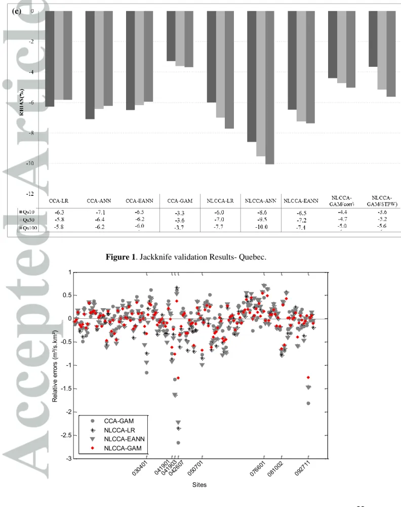
4.1. Results of the Quebec case study
The obtained results for the province of Quebec, using the cross-validation procedure for all considered combinations, are presented in Figure 1. Accordingly, the best overall performances
are those obtained from the full nonlinear model NLCCA-GAM first when the explanatory variables are those identified in Chokmani et Ouarda [2004], followed by the case when variables are selected with a stepwise technique (mainly in terms of RRMSE). In the following, we denote by NLCCA-GAM the model using BV, MBS, AMP, FAL and AMD variables. According to the high EC values (more than 0.8) and the lowest RRMSE values (28.35% for QS100), the
NLCCA-GAM model provides the most accurate estimates compared to all other approaches. Based on the RBIAS, results show that, even though all models underestimate flood quantiles, the CCA-GAM is the least biased model (-3.7 % for QS100). However, compared to the NLCCA-GAM approach,
the difference is not significant (a difference of -1.3 % for QS100).
Results indicate also that the NLCCA-GAM approach yields more accurate estimates when compared to the same approach using variables identified by stepwise, despite the fact that the difference is not too large. This may be explained by the fact that criteria used to select the variables (GCV and AIC) are not the same criteria used to evaluate model performances (EC, RRMSE, RBIAS). In addition, in the case of the stepwise based combination, the used NLCCA solution is the same as in the NLCCA-GAM. Hence, through a more advanced NLCCA parameterization, better results could be achieved by using the stepwise approach.
Moreover, the obtained results reveal that, when using the same gauged sites meaning the same delineation method, GAM outperforms ANN-based approaches (ANN and EANN) in terms of all evaluation criteria. This is probably attributable not only to the flexibility of GAM and its ability to adequately account for the nonlinearities, but also to the data size. Indeed, since the considered dataset is relatively not too large (151 catchments), the ANN-based models might not be properly trained. On the other hand, an expected finding is that, overall, the NLCCA-EANN approach outperforms ANN-based approaches (CCA-ANN, CCA-EANN and NLCCA-ANN). This is due
to the combination of the advantages of the nonlinear delineation method and the generalization ability of the nonlinear estimation method.
In addition, the gauged sites included in the homogeneous region when using the NLCCA approach lead to significant improvements in regional flood estimations when compared to sites retained using the linear CCA approach. More precisely, based on the RRMSE criterion (Figure 1-b), a relative improvement of 20% for the QS100 estimates is obtained when considering the
NLCCA-LR approach compared to the basic CCA-LR model. Regarding the estimation step, a relative improvement of 22% is recorded when considering CCA-GAM, and only 7% when considering the CCA-EANN approach. However, when we account for nonlinearity in both RFA steps, especially NLCCA combined with GAM, the relative gain reaches 45% (compared to the full linear model CCA-LR). This illustrates clearly the importance of the proposed approaches based on nonlinear tools in both RFA steps. In fact, an improvement in the estimation accuracy of quantiles at ungauged sites would significantly reduce flood damages, losses and costs.
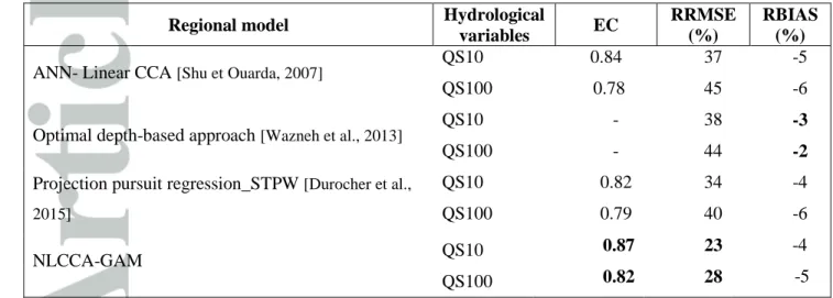
The comparison can also be extended to other regional models in the literature, such as the depth-based approach [Wazneh et al., 2013], the EANN in the CCA space [Shu et Ouarda, 2007; Khalil et al., 2011] and the projection pursuit regression approach [Durocher et al., 2015]. In the two latter approaches the delineation step is not considered (one-step RFA models) and, in addition, the estimation models are nonlinear. Table 3 reports the results of the above-listed studies. It indicates that, in terms of RRMSE and EC, the NLCCA-GAM model outperforms considerably all other approaches. However, the RBIAS values indicate that the depth-based approach performs slightly better.
To further explain the above results, the relative errors over sites associated to the best model in each category of combinations, CCA-GAM, NLCCA-LR, NLCCA-EANN and NLCCA-GAM,
are presented in Figure 2. One can notice that the lowest errors are associated to the full nonlinear combination NLCCA-GAM. Note also that, for some sites, the NLCCA-LR and NLCCA-EANN approaches show comparable performances. Furthermore, for a small number of sites the CCA-GAM approach seems to perform poorly. Indeed, a number of problematic stations corresponding to atypically large relative errors for most of the considered approaches have been identified (stations with identification numbers: 030401, 041901, 041903, 042607, 050701, 076601, 081002 and 092711). Some of these stations (030401, 041903 and 042607) were also identified in previous studies treating the same case study [Chokmani et Ouarda, 2004; Durocher et al., 2015]. These sites were found to have under-evaluated areas (Chokmani and Ouarda 2004). Using the NLCCA-GAM approach, the estimations corresponding to these particular sites are significantly improved as shown in Figure 2.
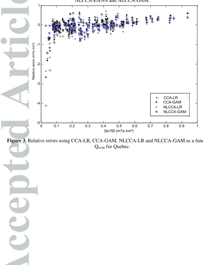
On the other hand, the exploration of the variability of errors as a function of the at-site QS100 is
shown in Figure 3 (because of space limitations and the similarity between results, those corresponding to QS10 and QS50 are not presented). One can see that the lowest specific quantile
values are poorly estimated by all approaches except when using the full nonlinear combination, NLCCA-GAM, which provides accurate estimates.
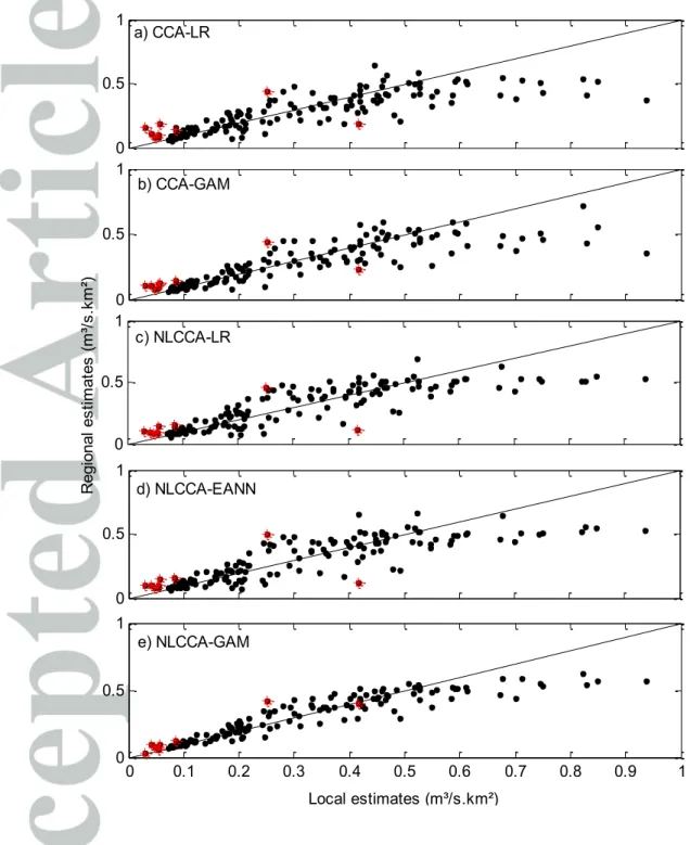
At-site versus regional quantile estimates are presented in Figure 4 for QS100. To this end, five
models are considered (CCA-LR, LR, EANN, CCA-GAM, and NLCCA-GAM) where LR-based ones (CCA-LR and NLCCA-LR) are considered as benchmarks and the NLCCA-EANN is selected as the best ANN-based model. According to Figure 4 the full nonlinear models show better overall performances (GAM followed by NLCCA-EANN). Indeed, associated at-site and regional estimations are very close since the points are less dispersed around the diagonal line. Moreover, higher specific quantile values are somewhat
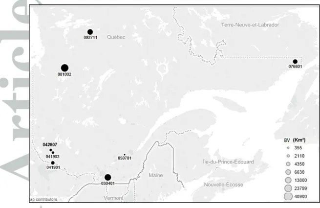
were found to be associated to small basins (the area is less than 800 km²), which seems to be systematically explained by their sharp hydrological responses. On the other hand, one can see, again, that the lowest specific quantile values are often overestimated except when using the full nonlinear model, NLCCA-GAM, by which they are well estimated. Note that these sites are the same ones identified as problematic in Figure 2. These sites, whose geographical locations are indicated in Figure 5, were found to have large basin areas (such as sites 030401, 076601, 081002 and 092711) or to be located in the limit of the province with medium size catchments (041901, 041903, 042607 and 050701).
As opposed to previous studies, where problematic sites were often removed to improve the model and the overall estimation results, in this work these stations are preserved. Figure 6 shows specifically relative errors for these sites. It indicates that the NLCCA-GAM model yields the best estimations for these particular sites and significant improvements are obtained which explain the overall high performance. In particular, the NLCCA-GAM model leads to an accurate estimate at the site 042607 which is the most notable station in previous studies and models. This site belongs to the drainage basin of the Kipawa River with a moderate catchment area of 2110 km2. Examination of the at-site estimation quantiles shows that this site has the lowest at-site quantile values for all return periods (64 m³/s for QS100). Hence, unlike the classical regressive
models, the high flexibility offered by GAM leads to a better modelling of the complex hydrological phenomena and to a much improved estimation. This finding points out a significant advantage of nonlinear models, in particular the NLCCA-GAM approach. Indeed, it shows that there is no need to develop specific models for different classes of basins according to their size, slope, or streamflow magnitude.
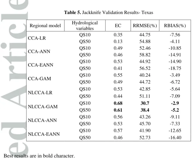
4.2. Results of the Arkansas and Texas case studies
Results of the Arkansas and Texas case studies are presented in Tables 4 and 5. It can be seen that, again, the NLCCA-GAM approach provides the most accurate estimates especially in terms of RRMSE. In fact, for Texas, the NLCCA-GAM performs well in terms of all evaluation criteria. However, the relative improvement was not as large as in the case of the province of Quebec. Indeed, the comparison of NLCCA-GAM and CCA-LR shows that a relative improvement of only 31% has been achieved in Texas for QS10 against 48% in the case of
Quebec. Results associated to Arkansas reveal that the NLCCA-GAM approach is recommended when considering the RRMSE which is the most important criterion [Hosking et Wallis, 1997]. Compared to the fully linear combination, the relative improvement reaches 35% for QS10. This
large difference between the NLCCA-GAM results in the three considered case studies can be explained by the fact that the nonlinearity is not as pronounced in the Arkansas and Texas case studies as it is the case of Quebec.
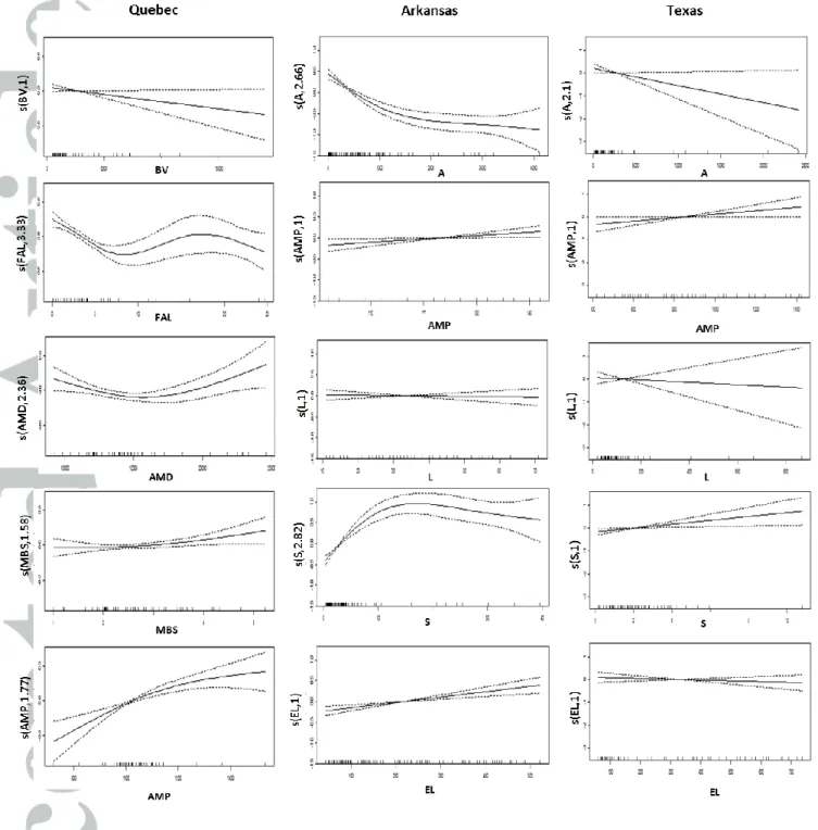
Figure 7 illustrates the smooth functions of the response variables as a function of the explanatory variables for the three considered case studies. One can effectively notice the difference in the degree of nonlinearity between the three regions. Indeed, the most complex relations between explanatory and response variables appear in the case of the province of Quebec which explains the high gain recorded when using the fully nonlinear combination NLCCA-GAM (48%). Note also, from these figures, that the Texas region seems to represent the simplest linear case study (linear smooth function curves and low edf values) which justify the smallest relative improvement (31%).
The main objective of this study is to investigate the potential of nonlinear approaches in both RFA steps, simultaneously. This allows taking full advantages of the nonlinearity considered in one of the two steps. To this end, a number of combinations of delineation methods (CCA and NLCCA) and regional estimation methods (LR, GAM, ANN and EANN) are considered. To illustrate the potential of the proposed approaches, these latter were applied to three different case studies in North America.
The obtained results reveal that considering nonlinear techniques in both RFA steps would significantly improve the performance of the regional model and, consequently, engender more accurate flood quantiles estimations at ungauged sites. This can have positive implications for the risk assessment of extreme hydrological events. In fact, the regional model combining the NLCCA approach for the delineation step with the GAM for the estimation step (NLCCA-GAM) was found to be the most appropriate model followed by the NLCCA-EANN approach for the Quebec case study.
Another noteworthy result is related to the importance of considering nonlinearity in the delineation or in the estimation step. It was found that considering nonlinearity in the delineation or in the estimation step lead to comparable results. Indeed, improvement in the overall model performance requires the integration of nonlinear tools in both steps. In summary, despite the relative complexity of the NLCCA-GAM approach, it is worthwhile to consider such model to adequately account for the nonlinearities of complex hydrological phenomena. Actually, a reliable regional model could be particularly useful for water resources managers.
In this study, the focus was on assessing the performances of the ANN and GAM models, combined to the NLCCA approach. In further efforts, it may be of interest to proceed with other
statistical techniques such as the projection pursuit regression, as a generalization of these two techniques, coupled to a delineation approach.
Acknowledgments
The authors thank Claude Onikpo for his valuable help and input. Financial support for the present study was graciously provided by the Natural Sciences and Engineering Research Council of Canada (NSERC). To get access to the data used in this study, reader may refer to the report of A. Kouider (http://espace.inrs.ca/365/1/T000342.pdf).
References
Abdi, A., Y. Hassanzadeh, S. Talatahari, A. Fakheri-Fard and R. Mirabbasi (2016). "Regional bivariate modeling of droughts using L-comoments and copulas." Stochastic Environmental Research and Risk Assessment: 1-12.
Agrafiotis, D. K., W. Cedeno and V. S. Lobanov (2002). "On the use of neural network ensembles in QSAR and QSPR." Journal of chemical information and computer sciences 42(4): 903-911.
Alobaidi, M. H., P. R. Marpu, T. B. M. J. Ouarda and F. Chebana (2015). "Regional frequency analysis at ungauged sites using a two-stage resampling generalized ensemble framework." Advances in Water Resources 84 103-111.
Anmala, J., O. W. Meier, A. J. Meier and S. Grubbs (2014). "GIS and Artificial Neural Network– Based Water Quality Model for a Stream Network in the Upper Green River Basin, Kentucky, USA." Journal of Environmental Engineering 141(5): 04014082.
Araghinejad, S., M. Azmi and M. Kholghi (2011). "Application of artificial neural network ensembles in probabilistic hydrological forecasting." Journal of Hydrology 407(1): 94-104. Ashtiani, A., P. A. Mirzaei and F. Haghighat (2014). "Indoor thermal condition in urban heat island: Comparison of the artificial neural network and regression methods prediction." Energy and Buildings 76: 597-604.
Austin, P. C. (2007). "A comparison of regression trees, logistic regression, generalized additive models, and multivariate adaptive regression splines for predicting AMI mortality." Statistics in medicine 26(15): 2937-2957.
Aziz, K., A. Rahman, G. Fang and S. Shrestha (2014). "Application of artificial neural networks in regional flood frequency analysis: a case study for Australia." Stochastic Environmental Research and Risk Assessment 28(3): 541-554.
Benzer, R. and S. Benzer (2015). "Application of artificial neural network into the freshwater fish caught in Turkey." 2(5): 341-346.
Besaw, L. E., D. M. Rizzo, P. R. Bierman and W. R. Hackett (2010). "Advances in ungauged streamflow prediction using artificial neural networks." Journal of Hydrology 386(1): 27-37. Bishop, C. M. (1995). Neural networks for pattern recognition, Oxford university press. Breiman, L. (1996). "Bagging predictors." Machine learning 24(2): 123-140.
Cannon, A. J. and P. H. Whitfield (2002). "Downscaling recent streamflow conditions in British Columbia, Canada using ensemble neural network models." Journal of Hydrology 259(1): 136-151.
Chebana, F., C. Charron, T. B. M. J. Ouarda and B. Martel (2014). "Regional Frequency Analysis at Ungauged Sites with the Generalized Additive Model." Journal of Hydrometeorology 15(6): 2418-2428.
Chen, P.-A., L.-C. Chang and F.-J. Chang (2013). "Reinforced recurrent neural networks for multi-step-ahead flood forecasts." Journal of Hydrology 497: 71-79.
Chokmani, K. and T. B. M. J. Ouarda (2004). "Physiographical space‐based kriging for regional flood frequency estimation at ungauged sites." Water Resources Research 40(12).
Chokmani, K., T. B. M. J. Ouarda, S. Hamilton, M. H. Ghedira and H. Gingras (2008). "Comparison of ice-affected streamflow estimates computed using artificial neural networks and multiple regression techniques." Journal of Hydrology 349(3): 383-396.
Coad, P., B. Cathers, J. E. Ball and R. Kadluczka (2014). "Proactive management of estuarine algal blooms using an automated monitoring buoy coupled with an artificial neural network." Environmental Modelling & Software 61: 393-409.
Dawson, C. and R. Wilby (2001). "Hydrological modelling using artificial neural networks." Progress in physical Geography 25(1): 80-108.
Dawson, C. W., R. J. Abrahart, A. Y. Shamseldin and R. L. Wilby (2006). "Flood estimation at ungauged sites using artificial neural networks." Journal of Hydrology 319(1): 391-409.
Demirel, M. C., M. Booij and A. Hoekstra (2015). "The skill of seasonal ensemble low-flow forecasts in the Moselle River for three different hydrological models." Hydrological Earth System Science 19: 275–291.
Durocher, M., F. Chebana and T. B. M. J. Ouarda (2015). "A Nonlinear Approach to Regional Flood Frequency Analysis Using Projection Pursuit Regression." Journal of Hydrometeorology
16(4): 1561-1574.
Eissa, Y., P. R. Marpu, I. Gherboudj, H. Ghedira, T. B. M. J. Ouarda and M. Chiesa (2013). "Artificial neural network based model for retrieval of the direct normal, diffuse horizontal and global horizontal irradiances using SEVIRI images." Solar Energy 89: 1-16.
Gao, C., M. Gemmer, X. Zeng, B. Liu, B. Su and Y. Wen (2010). "Projected streamflow in the Huaihe River Basin (2010–2100) using artificial neural network." Stochastic Environmental Research and Risk Assessment 24(5): 685-697.
Guisan, A., T. C. Edwards and T. Hastie (2002). "Generalized linear and generalized additive models in studies of species distributions: setting the scene." Ecological modelling 157(2): 89-100.
Hall, M. and A. Minns (1998). Regional flood frequency analysis using artificial neural networks. Hydroinformatics Conference. V. B. C. L. Larsen. Copenhagen, Denmark, A.A.Balkema. 2: 759– 763.
Hassanzadeh, Y., A. Abdi, S. Talatahari and V. P. Singh (2011). "Meta-heuristic algorithms for hydrologic frequency analysis." Water Resources Management 25(7): 1855-1879.
Hastie, T. and R. Tibshirani (1986). "Generalized additive models." Statistical science: 297-310. Hastie, T. J. and R. J. Tibshirani (1990). Generalized additive models, CRC Press.
Haykin, S. and R. Lippmann (1994). "Neural Networks, A Comprehensive Foundation." International Journal of Neural Systems 5(4): 363-364.
Hosking, J. and J. Wallis (1997). Regional Frequency Analysis. An Approach Based on L– moments. Cambridge, United Kingdom., Cambridge University Press. .
Hsieh, W. W. (2000). "Nonlinear canonical correlation analysis by neural networks." Neural Networks 13: 1095 -1105.
Huo, Z., S. Feng, S. Kang, G. Huang, F. Wang and P. Guo (2012). "Integrated neural networks for monthly river flow estimation in arid inland basin of Northwest China." Journal of Hydrology
Khalil, B., T. B. M. J. Ouarda and A. St-Hilaire (2011). "Estimation of water quality characteristics at ungauged sites using artificial neural networks and canonical correlation analysis." Journal of Hydrology 405(3): 277-287.
Kia, M. B., S. Pirasteh, B. Pradhan, A. R. Mahmud, W. N. A. Sulaiman and A. Moradi (2012). "An artificial neural network model for flood simulation using GIS: Johor River Basin, Malaysia." Environmental Earth Sciences 67(1): 251-264.
Kumar, R., N. K. Goel, C. Chatterjee and P. C. Nayak (2015). "Regional Flood Frequency Analysis using Soft Computing Techniques." Water Resources Management 29(6): 1965-1978. Lin, G.-F. and L.-H. Chen (2006). "Identification of homogeneous regions for regional frequency analysis using the self-organizing map." Journal of Hydrology 324(1): 1-9.
López‐Moreno, J. I. and D. Nogués‐Bravo (2005). "A generalized additive model for the spatial distribution of snowpack in the Spanish Pyrenees." Hydrological Processes 19(16): 3167-3176. McCullagh, P. and J. A. Nelder (1989). Generalized linear models, CRC press.
Nohair, M., A. St-Hilaire and T. B. M. J. Ouarda (2008). "The Bayesian-Regularized neural network approach to model daily water temperature in a small stream." Revue des sciences de l'eau 21(3).
Ouali, D., F. Chebana and T. B. M. J. Ouarda (2015). "Non-linear canonical correlation analysis in regional frequency analysis." Stochastic Environmental Research and Risk Assessment: 1-14. Ouarda, T. B. M. J., C. Girard, G. S. Cavadias and B. Bobée (2001). "Regional flood frequency estimation with canonical correlation analysis." Journal of Hydrology 254(1): 157-173.
Ouarda, T. B. M. J., M. Haché, P. Bruneau and B. Bobée (2000). "Regional flood peak and volume estimation in northern Canadian basin." Journal of Cold Regions Engineering 14(4): 176-191.
Ouarda, T. B. M. J. and C. Shu (2009). "Regional low-flow frequency analysis using single and ensemble artificial neural networks." Water Resources Research 45(11).
Pandey, G. and V. T. V. Nguyen (1999). "A comparative study of regression based methods in regional flood frequency analysis." Journal of Hydrology 225(1): 92-101.
Park, D. C., M. El-Sharkawi, R. Marks, L. Atlas and M. Damborg (1991). "Electric load forecasting using an artificial neural network." IEEE transactions on Power Systems 6(2): 442-449.
Pramanik, N. and R. K. Panda (2009). "Application of neural network and adaptive neuro-fuzzy inference systems for river flow prediction." Hydrological Sciences Journal 54(2): 247-260. Rumelhart, D., G. Hinton and R. Williams (1985). "Learning internal representations by error propagation " CALIFORNIA UNIV SAN DIEGO LA JOLLA INST FOR COGNITIVE SCIENCE.
Schwenk, H. and Y. Bengio (2000). "Boosting neural networks." Neural Computation 12(8): 1869-1887.
Seidou, O., T. B. M. J. Ouarda, L. Bilodeau, M. Hessami, A. St‐Hilaire and P. Bruneau (2006). "Modeling ice growth on Canadian lakes using artificial neural networks." Water Resources Research 42(11).
Shu, C. and D. H. Burn (2004). "Artificial neural network ensembles and their application in pooled flood frequency analysis." Water Resources Research 40(9).
Shu, C. and T. B. M. J. Ouarda (2007). "Flood frequency analysis at ungauged sites using artificial neural networks in canonical correlation analysis physiographic space." Water Resources Research 43(07).
Shu, C. and T. B. M. J. Ouarda (2008). "Regional flood frequency analysis at ungauged sites using the adaptive neuro-fuzzy inference system." Journal of Hydrology 349: 31– 43.
Sivakumar, B. and V. Singh (2012). "Hydrologic system complexity and nonlinear dynamic concepts for a catchment classification framework." Hydrology and Earth System Sciences
16(11): 4119-4131.
Taylan, P., G.-W. Weber and A. Beck (2007). "New approaches to regression by generalized additive models and continuous optimization for modern applications in finance, science and technology." Optimization 56(5-6): 675-698.
Wahba, G. (1990). Spline models for observational data. Philadelphia, SIAM.
Wang, W.-c., K.-w. Chau, L. Qiu and Y.-b. Chen (2015). "Improving forecasting accuracy of medium and long-term runoff using artificial neural network based on EEMD decomposition." Environmental research 139: 46-54.
Wazneh, H., F. Chebana and T. B. M. J. Ouarda (2013). "Optimal depth-based regional frequency analysis." Hydrology and Earth System Sciences 17(6): 2281-2296.
Werbos, P. J. (1994). The roots of backpropagation: from ordered derivatives to neural networks and political forecasting, John Wiley & Sons.
Wolpert, D. H. (1992). "Stacked generalization." Neural networks 5(2): 241-259. Wood, S. (2006). Generalized additive models: an introduction with R, CRC press.
Wood, S. N. (2003). "Thin plate regression splines." Journal of the Royal Statistical Society: Series B (Statistical Methodology) 65(1): 95-114.
Wu, C. and K. Chau (2011). "Rainfall–runoff modeling using artificial neural network coupled with singular spectrum analysis." Journal of Hydrology 399(3): 394-409.
Zaier, I., C. Shu, T. B. M. J. Ouarda, O. Seidou and F. Chebana (2010). "Estimation of ice thickness on lakes using artificial neural network ensembles." Journal of Hydrology 383(3): 330-340.
Zhang, B. and R. S. Govindaraju (2003). "Geomorphology-based artificial neural networks (GANNs) for estimation of direct runoff over watersheds." Journal of Hydrology 273(1): 18-34.
List of tables
Table 1. Descriptive statistics of hydrological and physio-meteorological variables-Quebec ... 27 Table 2. Summary of all considered regional models. ... 27 Table 3. Comparison of NLCCA-GAM with a number of RFA approaches from previous studies applied to the same dataset, Quebec. ... 28 Table 4. Jackknife Validation Results- Arkansas. ... 28 Table 5. Jackknife Validation Results- Texas ... 29
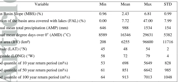
Table 1. Descriptive statistics of hydrological and physio-meteorological variables-Quebec
Variable Min Mean Max STD
Mean Basin Slope (MBS) (%) 0.96 2.43 6.81 0.99
Fraction of the basin area covered with lakes (FAL) (%) 0.00 7.72 47.00 7.99
Annual mean total precipitation (AMP) (mm) 646 988 1534 154
Annual mean degree days over 0o (AMD) (o C) 8589 16346 29631 5382
Basin area (BV) (km²) 208 6255 96600 11716
Latitude (LAT) (°N) 45 48 54 2
Longitude (LONG) (°W) 58 72 79 4
Flood quantile of 10 year return period (m³/s) 53 698 5649 828 Flood quantile of 50 year return period (m³/s) 61 851 6642 985 Flood quantile of 100 year return period (m³/s) 64 913 7013 1048
Table 2. Summary of all considered regional models. Delineation step (D) Estimation step (E) Regional model notation Reference Physiographical variables
Linear D & E CCA LR CCA-LR Ouarda et al. [2001] BV, MBS, FAL,
AMP, AMD
Linear D & nonlinear E
CCA ANN CCA-ANN
Current work BV, MBS, FAL, AMP, AMD
CCA EANN CCA-EANN
CCA GAM CCA-GAM Chebana et al. [2014]
Nonlinear D & linear E NLCCA LR NLCCA-LR Ouali et al. [2015] BV, MBS, FAL,
AMP, AMD
Nonlinear D & E
NLCCA ANN NLCCA-ANN
Current work
BV, MBS, FAL, AMP, AMD
NLCCA EANN NLCCA-EANN
NLCCA GAM NLCCA-GAM
NLCCA GAM
NLCCA-GAM/STPW
BV, FAL, AMD, LAT, LONG
Table 3. Comparison of NLCCA-GAM with a number of RFA approaches from previous studies applied
to the same dataset, Quebec.
Regional model Hydrological
variables EC
RRMSE (%)
RBIAS (%)
ANN- Linear CCA [Shu et Ouarda, 2007] QS10 QS100 0.84 0.78 37 45 -5 -6 Optimal depth-based approach [Wazneh et al., 2013]
QS10 QS100 - - 38 44 -3 -2
Projection pursuit regression_STPW [Durocher et al., 2015] QS10 QS100 0.82 0.79 34 40 -4 -6 NLCCA-GAM QS10 0.87 23 -4 QS100 0.82 28 -5
Best results are in bold character.
Table 4. Jackknife Validation Results- Arkansas.
Best results are in bold character.
Regional model Hydrological
variables EC RRMSE (%) RBIAS (%)
CCA-LR QS10 0.75 47.70 -3.04 QS50 0.73 61.36 -5.76 CCA-ANN QS10 0.71 63.58 -19.35 QS50 0.71 66.27 -14.80 CCA-EANN QS10 0.74 61.63 -16.83 QS50 0.73 68.97 -19.12 CCA-GAM QS10 0.74 40.54 -10.39 QS50 0.72 52.37 -13.50 NLCCA-LR QS10 0.72 37.23 6.27 QS50 0.71 44.78 5.54 NLCCA-GAM QS10 0.73 31.10 8.70 QS50 0.72 34.50 8.40 NLCCA-ANN QS10 0.65 49.71 8.16 QS50 0.67 51.30 2.71 NLCCA-EANN QS10 0.69 41.35 4.14 QS50 0.70 45.93 3.66
Table 5. Jackknife Validation Results- Texas
Best results are in bold character.
Regional model Hydrological
variables EC RRMSE(%) RBIAS(%)
CCA-LR QS10 0.35 44.75 -7.56 QS50 0.13 54.88 -4.11 CCA-ANN QS10 0.49 52.46 -10.85 QS50 0.46 58.82 -14.91 CCA-EANN QS10 0.53 44.92 -14.90 QS50 0.41 56.52 -18.75 CCA-GAM QS10 0.55 40.24 -3.49 QS50 0.49 44.72 -6.72 NLCCA-LR QS10 0.53 42.85 -5.64 QS50 0.44 51.11 -7.09 NLCCA-GAM QS10 0.68 30.7 -2.9 QS50 0.61 38.4 -5.2 NLCCA-ANN QS10 0.56 43.26 -9.11 QS50 0.53 45.70 -7.33 NLCCA-EANN QS10 0.57 41.90 -12.65 QS50 0.46 52.73 -16.40
List of Figures
Figure 1. Jackknife validation Results- Quebec. ... 32 Figure 2. Relative errors associated to QS100 calculated ateach site using CCA-GAM,
NLCCA-LR, NLCCA-EANN and NLCCA-GAM. ... 33 Figure 3. Relative errors using CCA-LR, CCA-GAM, NLCCA-LR and NLCCA-GAM as a function of QS100 for Quebec. ... 33
Figure 4. Jackknife estimation using the CCA-LR, CCA-GAM, NLCCA-LR, NLCCA-EANN, and the NLCCA-GAM approaches for QS100. Red asterisks are associated to estimations at
particular sites. ... 34 Figure 5. Geographical location of the identified particular stations in southern Quebec, Canada ... 35 Figure 6. Relative errors for identified problematic sites using several approaches, QS100. ... 35
Figure 7. Smooth functions of QS10 as a function of the explanatory variables of the
NLCCA-GAM model for Quebec, Arkansas and Texas, with associated 95% confidence intervals (dotted lines) and the estimated degree of freedom of the smooth (labelled in the vertical axes). ... 36
(a)
Figure 1. Jackknife validation Results- Quebec. -3 -2.5 -2 -1.5 -1 -0.5 0 0.5 1 Sites R el at iv e er ro rs (m ³/s .k m ²) 0426 07 0766 01 0304 01 0419 03 0810 02 0419 01 0507 01 0927 11 CCA-GAM NLCCA-LR NLCCA-EANN NLCCA-GAM (c)
Figure 2. Relative errors associated to QS100 calculated ateach site using CCA-GAM, NLCCA-LR, NLCCA-EANN and NLCCA-GAM.
Figure 3. Relative errors using CCA-LR, CCA-GAM, NLCCA-LR and NLCCA-GAM as a function of
QS100 for Quebec. 0 0.1 0.2 0.3 0.4 0.5 0.6 0.7 0.8 0.9 1 -5 -4 -3 -2 -1 0 1 Qs100 Qs100 (m³/s.km²) re la tiv e er ro r NLCCA-GAM CCA-GAM NLCCA-LR CCA-LR
D
0 0.1 0.2 0.3 0.4 0.5 0.6 0.7 0.8 0.9 1 -5 -4 -3 -2 -1 0 1 Qs100 Qs100 (m³/s.km²) re la tiv e er ro r NLCCA-GAM CCA-GAM NLCCA-LR CCA-LR 0 0.1 0.2 0.3 0.4 0.5 0.6 0.7 0.8 0.9 1 -5 -4 -3 -2 -1 0 1 Qs100 Qs100 (m³/s.km²) re la tiv e er ro r NLCCA-GAM CCA-GAM NLCCA-LR CCA-LR 0 0.1 0.2 0.3 0.4 0.5 0.6 0.7 0.8 0.9 1 -5 -4 -3 -2 -1 0 1 Qs100 Qs100 (m³/s.km²) re la tiv e er ro r NLCCA-GAM CCA-GAM NLCCA-LR CCA-LR 0 0.1 0.2 0.3 0.4 0.5 0.6 0.7 0.8 0.9 1 -5 -4 -3 -2 -1 0 1 Qs100 Qs100 (m³/s.km²) re la tiv e er ro r NLCCA-GAM CCA-GAM NLCCA-LR CCA-LR -3 -2.5 -2 -1.5 -1 -0.5 0 0.5 1 Sites R el at iv e er ro rs (m ³/s .k m ²) 0426 07 0766 01 0304 01 0419 03 0810 02 0419 01 0507 01 0927 11 CCA-GAM NLCCA-LR NLCCA-EANN NLCCA-GAMFigure 4. Jackknife estimation using the CCA-LR, CCA-GAM, NLCCA-LR, NLCCA-EANN, and the
NLCCA-GAM approaches for QS100. Red asterisks are associated to estimations at particular sites. 0 0.5 1 d) NLCCA-EANN 0 0.1 0.2 0.3 0.4 0.5 0.6 0.7 0.8 0.9 1 0 0.5 1 e) NLCCA-GAM R eg io na l e st im at es (m ³/s .k m ²) 0 0.5 1 b) CCA-GAM 0 0.5 1 a) CCA-LR Local estimates (m³/s.km²) 0 0.5 1 c) NLCCA-LR
Figure 5. Geographical location of the identified particular stations in southern Quebec, Canada
Figure 6. Relative errors for identified problematic sites using several approaches, QS100. Sites R el at iv e E rro rs (m ³/s .k m ²) 46 62 64 66 81 120 131 148 -4.5 -4 -3.5 -3 -2.5 -2 -1.5 -1 -0.5 0 0.5 1 NLCCA-ENN NLCCA-LR CCA-GAM CCA-LR NLCCA-GAM 092711 081002 076601 050701 042607 041903 041901 030401
Figure 7. Smooth functions of QS10 as a function of the explanatory variables of the NLCCA-GAM model for Quebec, Arkansas and Texas, with associated 95% confidence intervals (dotted lines) and the