Study of a Passive Companion Micro-Satellite to the SAOCOM-1B
Satellite of Argentina, for Bistatic and Interferometric SAR
Applications
Christian Barbier*
a, Dominique Derauw
a, Anne Orban
a, Malcolm W.J. Davidson**
b aCentre Spatial de Liège, Signal Processing Laboratory, Avenue du Pré-Aily, B-4031 Angleur
(Belgium);
bEuropean Space Agency, Head of Campaigns Section, Mission Science Division,
Postbus 299, 2200 AG Noordwijk (The Netherlands)
ABSTRACT
We report the results of a preparatory study aimed at exploring candidate applications that could benefit from a passive micro-satellite accompanying the L-band SAOCOM-1B satellite of Argentina, and to carry out a limited demonstration, based on data acquired during ESA airborne campaigns, of selected applications. In a first step of the study, the potential applications were identified and prioritized based on the mission context and strategic applications, scientific need, and feasibility. The next step of the study was to carry out some demonstrations using data sets acquired during the BioSAR 2007-2009, TropiSAR 2009 and IceSAR 2007 campaigns. A P-band InSAR digital elevation model was generated from BioSAR 2007 data. Time-series of interferometric coherence maps were obtained as a tool for change detection and monitoring. PolInSAR processing was carried out on BioSAR 2007 and IceSAR data.
Keywords: Synthetic Aperture Radar, SAR, SAOCOM, Bistatic SAR, InSAR, PolSAR, PolInSAR
1. INTRODUCTION
SAOCOM is an L-band, full-polarimetric SAR system to be deployed by Argentina in 2015 (SAOCOM-1A) and 2017 (SAOCOM-1B)1. The two satellites shall be part of the SIASGE disaster management constellation that also includes the X-band Cosmo-Skymed satellites. The main driver of the SAOCOM mission is the determination of soil moisture over an area that includes the Pampas region and the catchments from the fraction of the del Plata Basin (≈ 83000000 ha), which is the main Argentinean region dedicated to agriculture and cattle production, hence its major socio-economic value. The planned launcher, a Falcon 9, has an excess capacity with respect to SAOCOM. For the second SAOCOM spacecraft, CONAE has offered to ESA the possibility to use such excess capacity. In this context, ESA is exploring the technical feasibility and the scientific value of a bi-static extension of SAOCOM by means of a receive-only Companion Satellite (originally called SAOCOM-CS, now informally referred to as TANGOSat) flying in formation with the SAOCOM spacecraft, which would act as an illuminator2,3.
We report the results of a preparatory study aimed at exploring candidate applications that could benefit from a passive micro-satellite accompanying SAOCOM-1B, and to carry out a limited demonstration, based on data acquired during ESA airborne campaigns, of selected applications. In a first step of the study, the potential applications were identified and prioritized based on the mission context and strategic applications, scientific need, and feasibility. The next step of the study was to carry out some demonstrations using data sets acquired during the BioSAR 2007-2009, TropiSAR 2009 and IceSAR 2007 campaigns. A P-band InSAR digital elevation model was generated from BioSAR 2007 data. Time-series of interferometric coherence maps were obtained as a tool for change detection and monitoring. PolInSAR processing was carried out on BioSAR 2007 and IceSAR data.
This paper is structured as follows. The SAOCOM-1B and SAOCOM-CS missions are presented in Section 2. Section 3 offers an overview of coherence time monitoring, on which this paper is focused. Section 4 presents the results of the application demonstration carried out on P-band BioSAR 2007 data.
2. THE SAOCOM-CS MISSION
2.1 The SAOCOM project1
The SAOCOM system is made of two satellites that will be placed 180 degrees apart in a Sun-synchronous, nearly frozen polar orbit, with Local Time Ascending Node at 06:12 AM, at an altitude of 619.6 km and with a repeat cycle of 16 days (8 days with the full constellation). Both satellites shall be launched respectively in 2015 (SAOCOM-1A) and 2017 (SAOCOM-1B). The nominal mission duration shall be 5 years. The main payload of the two satellites shall be an L-band (1.275 GHz) fully polarimetric Synthetic Aperture Radar (SAR) providing High- (10 m) to Medium- (100 m) resolution imagery at incidence angles ranging from 23 to 50 degrees. This will be made possible thanks to an electronically steered phase antenna allowing multiple possibilities in terms of incidence angle, swath width, resolution, polarisation. Polarisation capabilities will include selectable single polarisation (SP), selectable double polarisation (DP), and full quad polarisation (QP). Compact polarisation (CL-POL), i.e., circular transmission, linear reception, shall be available as a technological mode. For high resolution, the images will be acquired in classical Stripmap (SM) at selected incidence angles and in SP, DP and QP. TOPSAR is used to increase swath width at the expense of resolution in SP, DP and QP. All these acquisition modes make use of a limited set (19) of optimized beams, i.e., 10 beams for QP with a maximum swath width of 220 km and 3 levels of resolution, and 9 beams for SP and DP allowing maximum coverage of 360 km and maximum access of 430 km and 3 levels of resolution. The SAR antenna shall be nominally right-looking with left-looking capability for limited periods of time in accordance with system resources. Yaw-steering will be implemented.
A Memorandum Of Understanding (MOU) was signed with the Italian Space Agency (ASI) to integrate the SAOCOM satellites into the SIASGE Risk Management System, that will also include the four COSMO-Skymed X-band SAR satellites already in orbit. It is expected that the combined system will generate X + L – band products with added value compared to separated X- and L-band products.
The main driver of the SAOCOM mission is the determination of soil moisture over an area that includes the Pampas region and the catchments from the fraction of the del Plata Basin (≈ 83000000 ha), which is the main Argentinean region dedicated to agriculture and cattle production, hence its major socio-economic value. There are three so-called strategic applications of soil moisture measurements over this region : (a) agriculture : to optimize the agrochemical use in crop disease control; (b) agriculture : to optimize sowing time and fertilizers; (c) hydrology : to minimize the losses due to floods in Argentina, and to optimize the protection works for future floods. The SAOCOM mission includes a baseline mission, a foreground mission and a background mission. The baseline mission will be dedicated to fixed acquisitions over the Pampa region for operational generation of soil moisture maps, as well as for calibration, mainly over the Rain Forest of the Amazon and specific point targets (transponders, corner reflectors). The foreground mission will consist of variable acquisitions over the ASI zone of interest mainly for emergencies (25°W-120°E longitude, 0°-80°N latitude), for maritime surveillance over the Argentinean sea, as well as any other user within or outside Argentina. Finally the background mission will aim at generating, according to available resources, an image database for future use over Argentina (emergencies, biomass), Latin America (plate and glacier movements in the Andes, biomass), and the rest of the world (biomass, calibration, change detection, maritime routes).
2.2 The SAOCOM-CS mission summary and timeline2,3
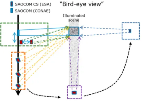
A major characteristic of missions with two or more SAR satellites flying in formation is that i) they can provide single-pass interferometric4-6 and tomographic7 measurements enabling a 3D radar view of the Earth’s vegetation layers, surface and near-surface interior, and ii) they allow for the systematic exploration of new applications based on bistatic interferometric and radiometric measurements. Accordingly, the science opportunities created by the SAOCOM-CS missions are dictated to a great extent by the geometrical position and orientation with respect to the main SAOCOM satellite during image acquisition. The main geometries considered for the mission are illustrated in Figure 1 and can be summarised as follows:
- Tomographic: characterised by short along-track baselines and variable across-track baselines, which are used
to build up a 3-dimensional view of the radar scattering surfaces (green box in Figure 1)
- Bistatic: subdivided into a bistatic geometry with large along-track displacement and zero across-track
- Specular: the companion satellite views the illuminated scene from the specular direction, i.e. mirror opposite
to the SAOCOM satellite (blue box).
Figure 1 (color online). Main SAOCOM-CS mission observation geometries3
Using these geometrical arrangements a timeline of science data takes was elaborated, which includes tomographic acquisition phases dedicated to boreal and tropical forest tomography and vegetation structure retrieval, subsurface mapping of ice and arid zones, bistatic interferometric measurements of urban environments and surface motion and bistatic radiometric characterisation of surface and vegetation scattering as well as new bistatic retrieval demonstration of soil moisture. In total the timeline includes ~4.8 years of science and is compatible with the expected lifetime of the mission and on-board propellant reserves.
The SAOCOM-CS reference orbit is the same as SAOCOM-1B: a Frozen Sun-Synchronous, dawn-dusk, 97.88° of inclination orbit with a 6:12 a.m. LTAN and a reference orbit altitude of 619.6 km. It will be flying in formation, leading SAOCOM-1B to avoid collision risks, with along-track distances ranging between 5 km and 250 km and across track distances from 0 km to 12 km depending on the scientific objective. It will be able to point to the centre of any of the first 4 swaths of SAOCOM when SAOCOM is operating in Stripmap mode (either in Dual of Full polarisation mode). SAOCOM-CS is designed to take side right looking measurements with an orbit duty cycle of 6 minutes during tomographic and bistatic application observations.
The payload of SAOCOM-CS consists of a passive deployable fix-beam L-band antenna originally developed for the LARSAR-TERRASAR-L and a fully redundant Payload Central Electronics assembly based on heritage from Sentinel-1, with transmit functionality removed and the centre frequency adapted to L-band. The payload has been designed as a receive-only instrument.
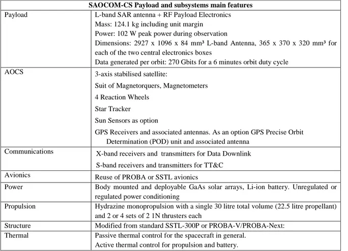
Two platform concepts are currently subject to Phase A/B1 concurrent studies : a PROBA-based concept and a SSTL-300P concept. Both concepts reuse the avionics with addition of extra mass memory to store the generated data. Scientific data is sent to ground via a 200-350 Mbit/s X-band data downlink. Table 1 collects the SAOCOM-CS payload and subsystem main characteristics. See Ref. 3 for more details and illustrations.
Table 1. SAOCOM-CS payload and subsystem main features3
SAOCOM-CS Payload and subsystems main features
Payload L-band SAR antenna + RF Payload Electronics Mass: 124.1 kg including unit margin
Power: 102 W peak power during observation
Dimensions: 2927 x 1096 x 84 mm³ L-band Antenna, 365 x 370 x 320 mm³ for each of the two central electronics boxes
Data generated per orbit: 270 Gbits for a 6 minutes orbit duty cycle
AOCS 3-axis stabilised satellite:
Suit of Magnetorquers, Magnetometers 4 Reaction Wheels
Star Tracker
Sun Sensors as option
GPS Receivers and associated antennas. As an option GPS Precise Orbit Determination (POD) unit and associated antenna
Communications X-band receivers and transmitters for Data Downlink S-band receivers and transmitters for TT&C
Avionics Reuse of PROBA or SSTL avionics
Power Body mounted and deployable GaAs solar arrays, Li-ion battery. Unregulated or regulated power conditioning
Propulsion Hydrazine monopropulsion with a single 30 litre total volume (22.5 litre propellant) and 2 or 4 sets of 2 1N thrusters each
Structure Modified from standard SSTL-300P or PROBA-V/PROBA-Next: Thermal Passive thermal control for the spacecraft in general.
Active thermal control for propulsion and battery.
3. COHERENCE TIME MONITORING
Single-pass InSAR is the most immediate application of a close formation-flying SAR constellation, because it involves no time-decorrelation. This was the original configuration proposed by Zebker and Goldstein in the airborne case4. It was implemented in space only recently, first in the short-duration STS-99 Shuttle Radar Topography Mission5, then in the still-going TanDEM-X mission6. The latter operates in X-band, but an L-band version, known as TanDEM-L, has been proposed, albeit with a broader scope than topographic mapping8.
A by product of any InSAR processor, beside the surface Digital Elevation Model (DEM), is the coherence map, which is a measure of the “inteferability” of the two image partners. Although zero coherence strictly speaking means “no interferability”, it can be a source of information by itself. As an example, during an ESA DUP study aiming at evaluating the quality of InSAR topographic mapping using ERS-1/2 Tandem pairs over Belgium (REF), some zones of low coherence over crop fields were found to be related to ploughing during the 24-hours lapse separating the two acquisitions9. Conversely, coherence-preserving zones may constitute indicators of, e.g., mine fields, and can be used for ground displacement detection.
Time series of coherence maps between ERS-1/2 Tandem pairs were used in a study to evaluate InSAR potentialities for crop identification and monitoring10. Although the results would deserve consolidation, it was found that time series of coherence maps might be used to differentiate between crop species and to monitor crop growth.
In another context, that of providing assistance to irrigation monitoring and management11, a study is being carried out under a PhD Thesis in collaboration between CSL, the Department of Environmental Sciences and Management of the University of Liège, the Institut National de Recherches Agronomiques of Morocco, using ERS-1/2 and ENVISAT data in the framework of a CAT-1 project accepted by ESA. The proposed activity aims at determining to what extent interferometric coherence can be used in complement to traditional VIS/NIR imagery to assist irrigation management in the Tadla region. The cereal has a significant place in production systems in Morocco12. It occupies 75% of the cultivated areas. The flood irrigation is the most common technique used up to 96% of the area. The efficiency of this technique is estimated at 50%. Since 2009, Morocco is making efforts for valuing and saving of irrigation water in order to prepare the Moroccan agricultural sector to the new demands, including climate change. These efforts can be supported by modernizing management practices in irrigation water resources.
In such contexts, it is clear that single-pass InSAR data from the SAOCOM-SAOCOM-CS system would provide an opportunity to extend and consolidate these investigations. The basic product is a time series of coherence maps obtained by standard InSAR processing of Single-Look Complex, Level 1A, image pairs. For a polarimetric system like SAOCOM-1B / SAOCOM-CS, there will be as many coherence maps per acquisition as there are polarization channels, i.e. one for single-pol, two for dual-pol and three for quad-pol. These coherence maps are Level 1A products and are registered on a standard reference grid to be defined. In the case of a full polarimetric acquisition, further Level 1A products, i.e., optimized coherences, can be obtained by PolInSAR processing. Other Level 1A products are to be defined, but could include colour composites showing coherence evolution over a 3-date time series of coherence maps. Higher-level products shall be defined and generated by the users.
Two scenarios can be envisaged to generate coherence maps :
- Coherence maps generated from single-pass InSAR combining one SAOCOM-1B image (monostatic) and one SAOCOM-CS (bistatic) image. The time series is built by repeating the single-pass acquisition process. This would be a generalisation of the CSL ERS-1/ERS-2 Tandem study.
- Coherence maps generated from double-pass SAOCOM-1B or SAOCOM-CS acquisitions.
4. APPLICATIONS DEMONSTRATIONS : COHERENCE MEASUREMENTS
4.1 Data sets and test site
We will concentrate on coherence measurements made on data sets from the ESA BioSAR 2007 airborne campaign.The data were acquired by the DLR E-SAR system. The test site was a fairly flat area covered by sparse forests, in Southern Sweden (Remningstorps). P-band interferometric pairs with short temporal baselines were acquired on March 9, April 2 and May 2, 2007. Similarly, L-band interferometric pairs with short temporal baselines were acquired on March 9, March 31 and May 2, 2007.
4.2 P-band DEM
ESAR being an airborne SAR system, the first step was to adapt the CSL InSAR suite, originally designed for processing spaceborne imagery, to this configuration. First, a “quick-and-dirty” ESAR data reader was developed. Only slant-range Single-Look Complex (SLC) (.rgi) data were considered for processing. Having been developed for spaceborne sensors, the CSL processor does not take motion compensation into account. A second important adaptation was required due the fact that ESAR is left-looking, while most spaceborne systems are right-looking. The net result of these modifications is an increase of the processor robustness.
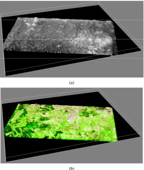
In order to test the modified processing chain, a Digital Elevation Model (DEM) was generated from the BioSAR2007 data set. The selected data pair is a full polarimetric P-Band data pair corresponding to acquisitions 0411 and 0407, both on May 2, 2007 with a time delay of approximately 5 hours. This interferometric pair is supposed to have a baseline (about 19 m) leading to an altitude ambiguity of approximately 100 m.After phase unwrapping, the DEM in slant range was issued, and all interferometric products were geoprojected in UTM coordinate on WGS84. Figure2 shows a three-dimensional representation of the derived DEM. The area being quite flat, with relief variation of about 25 m maximum on the whole observed zone, height variations have been largely exaggerated for visual aspect improvement.
(a)
(b)
Figure 2 (color online) : 3D view of the P-band DEM derived from BioSAR 2007 data set. (a): Gray level with respect to local height; (b): Color composition: Red = Coherence, Green = average intensity, Blue = Log of average intensity
4.3 Optimized coherences
PolInSAR coherence optimization leads to a decomposition of the observed scattering process into three principal elementary scattering processes, each of which having its own interferometric phase response and interferometric coherence13. Using Pauli matrix decomposition, the first elementary scattering process corresponds to surface scattering. The second elementary scattering process corresponds to dihedral response and the third one to volumetric (random) scattering process.
With respect to the BioSAR2007 P-band data set, we carried out PolInSAR processing of the three interferometric pairs 0306-0105 (April 2 – March 9), 0411-0105 (May 2 – March 9) and 0411-0301 (May 2 – April 2). We could obtain optimized coherence measurements at quasi null baselines (Bh~0m, Bv~3m) with time spans of 24, 30 and 54 days at different seasonal periods. This allowed us to analyze coherence evolution with time, while minimizing the contribution of geometrical decorrelation. Figure 3 shows the histogram of the three optimized coherences obtained for the PolInSAR pairs leading to a 24- and a 30-day time gap.
Figure 3 (color online) : Optimized interferometric coherence histograms for two time spans (24 and 30 days)
We observe that, whatever the optimized coherence, the shortest time gap leads to the largest coherence loss, while we should expect exactly the converse; in other words, coherence losses are not related to the time gap but to a seasonal effect. This can be also observed using other interferometric pairs in the same set. Considering pairs 0406, 0411-0306, 0301-0105 and 0411-0105, we can compute the histogram of coherence encompassing a time gap of 0, 24, 30 and 54 days at quasi null baseline.
This seasonal effect detected through histogram comparison reflects only a global behavior. We can observe more precise coherence variation making a colour composite image of estimated coherences. Figure 4 shows a color composite image using the 30-day coherence for the red channel (pair 0411-0301), the 54-day coherence for the green channel (pair 0411-0105) and the 24-day coherence for the blue channel (pair 0306-0105). The coherence channel used is the first optimized coherence issued through PolInSAR processing.
Although this kind of image is extremely difficult to interpret, we can extract some leading lines :
If the color composite is black, it means that coherence is low whatever the time gap. Consequently, we deal mainly with strong volume scattering. Therefore, black zones should probably correspond to forested areas. If the color is white, this means that coherence is preserved in any channel, whatever the time gap. This can be the case in urban zones or in bare dry soils areas. Dark blue areas correspond to zones losing coherence principally during April, keeping a good stability in March. Conversely, red areas are those losing more coherence in March than in April. Green areas correspond to zones recovering long term coherence (between March 9 and May 2), while losing it with respect to the April 2 acquisitions. We can also observe some yellow and cyan plots. Yellow corresponds to higher signal in the red and green channel. Cyan corresponds to higher signal in the green and blue channel.
Let us assume that coherence is an indicator of variation with respect to certain parameter or parameters : this (these) can be the humidity level, the foliage density, the roughness, etc. Coherence loss will then be linked to, or be an indicator of, the variation of the considered parameter. Graphically, we can then represent a constant high level of coherence (white zones in the image) and low level of coherence (black zones) as shown in the lower part of Figure 4. Low variations will induce few temporal decorrelation, hence high coherence. Conversely, higher variations will induce higher time decorrelation, hence lower coherence. Even if this representation is basic and simplistic, it shows that local coherence variation with time are linked to much finer variation inside the test site than solely a global seasonal variation as shown looking only to the histogram variations.
As far as the second and third optimized coherence channels issued through PolInSAR processing are concerned, the results are similar to the one represented in Figure 4, although more contrasted.
Figure 4 (color online): Color composite image and interpretation key of temporal coherence evolution with interpretation PolInSAR first optimized coherence channel).
The above analysis is confirmed by PolSAR analysis. We computed the respective amplitude of each of these elementary scattering processes within the scattering matrix and we generated entropy, anisotropy and alpha images (HAα decomposition) of each acquisition. Entropy gives information on the «purity» of the underlying backscattering process. If the entropy is low, one elementary scattering is predominant ; if it is high, the three elementary scattering processes are equiprobable and the medium is depolarizing. In conjunction with entropy, anisotropy allows precising the « purity » of the backscattering process : in case of null entropy, anisotropy allows determining which is the scattering process. When the scattering is a mix of processes, the alpha parameter allows determining which is the predominant scattering process. Entropy changes mean that backscattering processes evolve with time. If entropy increases, it means that we evolve from a situation with no predominant backscattering process to a situation with one predominant backscattering process. Conversely, if the entropy decreases, we evolve from a predominant backscattering process toward a mix of backscattering processes. If entropy stays constant, we can suppose that the backscattering processes stay stables. It is clearly observed that the zones subjected to backscattering changes are those losing nearly completely temporal coherence. This is logical : if backscattering process changes with time, we do not compare the same scatterer distribution. Consequently, phase coherence cannot be preserved. This also confirms the fact that temporal coherence changes are linked to global parameter changes, like humidity, affecting all scatterers in the same way. Temporal coherence evolution is clearly observed in zones showing stable entropy.
4.4 RVoG inversion
The Random Volume over Ground (RVoG) model [13] provides a useful way of interpreting the mixture of ground and vegetation. The model relies on the interferometric coherence evaluated for different polarization channels by the PolInSAR processing. In that case, the complex interferometric coherence is a combination of volume and surface scattering. Introducing the ground contribution into the vertical distribution function of scatterers leads to express the RVoG complex interferometric coherence by :
( )
( )
( )
( )
( )
( )
( )
(
)
−
+
=
+
+
=
vol volm
m
j
m
m
j
γ
ω
ω
ϕ
ω
ω
γ
ϕ
ω
γ
1
1
exp
1
exp
0 0 (1) where :( )
( )
( )
−
=
θ
σ
ω
ω
ω
cos
2
exp
v vol groundh
m
m
m
(2)is the ground-to-volume ratio for a vertical scattering center distribution with constant attenuation coefficient σ over hv.
It corresponds to the ratio of ground and volume radar cross sections, and defines the relative importance of both ground and volume contributions.
ω
defines the scattering mechanism, the interferometric coherence dependence on the polarization lying in the relative scattering interaction between the vegetation and the ground, through the factor .λ
π
ϕ
0=
4 R
0 is the underlying ground phase. Due to volume decorrelation, φ0 differs from the interferometric phase.The three PolInSAR optimized coherences correspond each to an independent scattering mechanism and the three interferograms provide to the mean location of the underlying mechanism center. These three scattering mechanisms are those maximizing the separation between interferometric phase centers, which theoretically corresponds to the largest available spectrum of m-values and provides then a better conditioning for RVoG model inversion for tree height retrieval.
Forest height inversion is based on the assumption that one of the measured channels is pure volume coherence . We use the third optimized coherence value but it can be selected following an a priori knowledge of the scene.
Evaluation of the contribution of volume decorrelation contribution is therefore a critical step in inverting the RVoG model and all the sources of non-volumetric decorrelation will cause error on the inverted heights. After correction of decorrelation effects induced by system, acquisition geometry and processing effects, temporal decorrelation contribution remains. Temporal decorrelation reduces the interferometric coherence and increases the variation of interferometric phase. It affects both volume component and underlying ground. It introduces a bias in forest height estimation due to coherence underestimation, in particular volume coherence. The amount of temporal decorrelation depends on the changing processes occurring during the time interval between acquisitions. Using a companion satellite would allow to overcome this problem by providing single-pass interferometric acquisitions.
Further to temporal decorrelation, two other important points for a performing RVoG inversion are: 1) the effective baseline or absolute interferometric wavenumber given by:
θ
λ
π
sin
θ
2
∆
=
zk
(3)2) the length of the best fit line through coherence values in the geometrical representation of the RVoG model, the line model being used to evaluate the ground phase φ0.
kz depends on the baseline and determines the ambiguity altitude ha. The choice of the baseline is essential in order to
perform meaningful height estimation. It has to be selected such that the altitude of ambiguity is between 1.2 and twice the maximum vegetation height hv: 1.2 hv < ha < 2 hv. The vegetation height in the observed area (boreal forest stands in
Remningstorps estate, in Southern of Sweden) is about 20-30 m, which corresponds to an optimum ha between 20 – 50 m
or 0.06 < |kz| < 0.14.
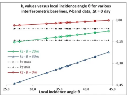
We performed RVoG inversion over a series of 14 regions of interest (ROI’s) in the observed area. For B = 20m, the effective baseline (or absolute kz value) is closer to its optimum value with respect to observed vegetation height: 0.06 <
|kz| < 0.14. This can be seen on Figure 5, showing the effective baseline values as a function of local incidence angle, for
the 14 ROI’s. It clearly appears that baseline of 0m and 60m are not convenient for tree height retrieval. The RVoG inversion on the 14 ROI’s is plotted in Figure 6. The results are in line with the Remningstorps forest average vegetation height of 20-30 meters.
5. CONCLUSIONS
This paper reported results from one of the scientific studies contracted by ESA to investigate and demonstrate the spectrum of applications made accessible by the SAOCOM-1B/SAOCOM-CS joint mission. We have addressed the particular topics of coherence time monitoring and shown, using full polarimetric interferometric P-band data sets from the BioSAR 2007, that this technique allows change monitoring at both global (seasonal) and local levels. This conclusion should be consolidated by new airborne campaigns, to be organized in the context of both SAOCOM-CS and BIOMASS missions.
6. ACKNOWLEDGEMENT
This work was carried out under ESA Contract Nr. 400109707/13/NL/FF/vb “OLIVIA : Study on applications of a passive European companion satellite to the CONAE SAOCOM mission”.
Figure 5 (color online) : kz value for BioSAR P-band data
REFERENCES
[1] See, for example, Frulla, L.A., Rodriguez Ortega, G. and Milovich, J.A., “CONAE’s SAR missions overview”, Proc. PIERS 2009, Moscow, Russia, 18-21 Aug. 2009.
[2] Davidson, M.W.J., Gebert, N., Carnicero Domínguez, B., Fois, F., Silvestrin, P. and Frulla, L., “A passive companion to SAOCOM for single-pass L-band SAR interferometry”, Proc. IGARSS 2014, Quebec, Canada, 13-18 July 2014.
[3] Carnicero Domínguez, B. Gebert, N., Davidson, M.W.J., Ludwig, M., van Pelt, M., Beyer, F., García Matatoros, M., de Vogeleer, B., Silvestrin, P., Wokes, S., Gerrits, D., Vrancken, D., Tallineau, J. and Saameño, P., “SAOCOM-CS: Developing a SAR companion satellite based on a small platform”, Proc. 4S[OA1] Symp. On Small Satellites and Systems, Majorca, Spain, 26-30 May 2014.
[4] (a) H.A. Zebker and R.M.Goldstein, “Topographic Mapping from Interferometric Synthetic Aperture Radar Observations”, J. Geophys. Res. 91(B5), 4993-4999 (1996); (b) for a general review, see : G. Krieger, I. Hajnsek, K. Papathanassiou, M. Younis, and A. Moreira, “Interferometric Synthetic Aperture Radar (SAR) Employing Formation Flying”, Proc. IEEE 98(5), 816-843 (2010).
[5] T.G. Farr, P.A. Rosen, E. Caro, R. Crippen, R. Duren, S. Hensley, M. Kobrick, M. Paller, E. Rodriguez, L. Roth, D. Seal, S. Shaffer, J. Shimada, J. Umland, M. Werner, M. Oskin, D. Burbank, and D. Alsdorf, “The Shuttle Radar Topography Mission”, Rev. Geophys., 45, RG2004 (2007); (b) B. Rabus, M. Eineder, A. Roth, and R. Bamler, “The Shuttle Radar Topography Mission- a New Class of Digital Elevation Models Acquired by Spaceborne Radar”, Photogramm. Rem. Sens. 57, 241-262 (2003).
[6] G. Krieger, A. Moreira, H. Fiedler, I. Hajnsek, M. Werner, M. Younis, and M. Zink, “TanDEM-X : A Satellite Formation for High-Resolution SAR Interferometry”, IEEE Trans. Geosci. Remote Sens. 45(11), 3317-3340 (2007).
[7] As a starting point, see (a) Reigber, A. and Moreira, A., “First demonstration of airborne SAR tomography using multibaseline L-band data”, IEEE Trans. Geosci. Remote Sens. 38, 2142-2152 (2000); (b) Fornaro, G., Lombardini, P. and Serafino,F., “Three-dimensional multipass SAR focusing : Experiments with long-term spaceborne data”, ibid. 43, 702-714 (2005).
[8] Krieger, G., Hajnsek, I., Papathanassiou, K., Eineder, M., Younis, M., De Zan, F., Prats, P., Huber, S., Fiedler, H., Freeman, A., Rosen, P., Hensley, S., Johnson, W., Veilleux, L., Grafmueller, B., Werninghaus, R., Bamler, R. and Moreira, A., “The TanDEM-L Mission Proposal : Monitoring Earth’s Dynamics with High Resolution SAR Interferometry”, Proc. IEEE Radar Conf. Passadena, CA, May 4-8 (2009).
[9] Derauw, D. and Barbier, C, “Quality assessment of InSAR topographic mapping : the example of Belgium”, Proc. SPIE 3497, 175-185 (1998).
[10]Blaes, X., Defourny, P., Derauw, D. and Barbier, C., “InSAR Coherence for Crop Parameter Monitoring”, Proc. FRINGE’99 Symp. Liège, 10-12 Nov. 1999, ESA SP-478.
[11]Ozdogan, M., Yang, Y., Allez, G. and Cervantes, C., « Remote Sensing of Irrigated Agriculture : Opportunities and Challenges » Remote Sensing 2, 2274-2304 (2010).
[12]Balaghi, R., Jlibene, M., Tychon, B. and Eerens, H., “La Prédiction Agrométéorologique des Rendements Céréaliers au Maroc”, Institut National de La Recherche Agronomique, Maroc (2012).
[13](a) Cloude, S.R. and Papathanassiou, K.P., « Polarimetric SAR Interferometry », IEEE Trans. Geosci. Remote Sens. 36(5), 1551-1565 (1998); (b) Papathanasiou, K.P. and Cloude, S.R., “Single-Baseline Polarimetric SAR Interferometry”, ibid. 39(11), 2352-2363 (2001);
[14]Treuhaft, R.N. and Siqueira, P.R., “The vertical structure of vegetated land surfaces from interferometric and polarimetric radar”, Radio Science 35, 141-177 (2000).