Pépite | Restitution des propriétés des nuages à partir des mesures multi-spectrales, multi-angulaires et polarisées du radiomètre aéroporté OSIRIS

Texte intégral

(1)Thèse de Christian Matar, Université de Lille, 2019. Restitution des Propriétés des Nuages à partir des Mesures Multi-Spectrales, Multi-Angulaires et Polarisées du Radiomètre Aéroporté OSIRIS. Thèse de Doctorat de. Christian MATAR Pour obtenir le grade de Docteur de l’Université de Lille Discipline: Optique et Lasers, Physico-Chimie de l’Atmosphère. _____________________________________________ Soutenue le 6 Mai 2019 devant le jury composé de:. Marjolaine CHIRIACO Rodolphe MARION Frédéric SZCZAP. Laboratoire Atmosphères, Milieux, Observations Spatiales Commissariat à l’Énergie Atomique et aux Énergies Alternatives Laboratoire de Météorologie Physique. Rapporteur Rapporteur Examinateur Examinateur. Fréderic PAROL. Laboratoire Atmosphères, Milieux, Observations Spatiales Laboratoire d’Optique Atmosphérique. Céline CORNET. Laboratoire d’Optique Atmosphérique. Co-directeur. Cyrille FLAMANT. Directeur. Laboratoire d’Optique Atmosphérique Faculté de Sciences et Technologies Université de Lille 59655 Villeneuve d’Ascq, France. © 2019 Tous droits réservés.. lilliad.univ-lille.fr.

(2) Thèse de Christian Matar, Université de Lille, 2019. © 2019 Tous droits réservés.. lilliad.univ-lille.fr.

(3) Thèse de Christian Matar, Université de Lille, 2019. Retrieval of Cloud Properties Using the Multi-Spectral, Multi-Angular and Polarized Measurements of the Airborne Radiometer OSIRIS. Doctoral Thesis of. Christian MATAR To obtain the grade of PhD from the University of Lille Discipline: Optics, Lasers, Physics and Chemistry of the Atmosphere. _____________________________________________ Defended in 6 May 2019 in front of the jury composed of:. Marjolaine CHIRIACO Rodolphe MARION Frédéric SZCZAP Cyrille FLAMANT. Laboratoire Atmosphères, Milieux, Observations Spatiales Commissariat à l’Énergie Atomique et aux Énergies Alternatives Laboratoire de Météorologie Physique. Reviewer Reviewer Examiner. Fréderic PAROL. Laboratoire Atmosphères, Milieux, Observations Spatiales Laboratoire d’Optique Atmosphérique. Supervisor. Céline CORNET. Laboratoire d’Optique Atmosphérique. Co-supervisor. Examiner. Laboratoire d’Optique Atmosphérique Faculté de Sciences et Technologies Université de Lille 59655 Villeneuve d’Ascq, France © 2019 Tous droits réservés.. lilliad.univ-lille.fr.




(7) Thèse de Christian Matar, Université de Lille, 2019. Abstract. Cloud feedbacks remain one of the major uncertainties of climate prediction models, particularly the interactions between aerosols, clouds and radiation (IPCC - Boucher et al., 2013). Clouds are indeed difficult to account for because they have significant spatial and temporal variability depending on a lot of meteorological variables and aerosol concentration. Airborne remote sensing measurements with tens of meters resolution are very suitable for improving and refining our knowledge of cloud properties and their high spatial variability. In this context, we exploit the multi-angular measurements of the new airborne radiometer OSIRIS (Observing System Including PolaRization in the Solar Infrared Spectrum), developed by the Laboratoire d'Optique Atmosphérique. It is based on the POLDER concept as a prototype of the future 3MI space instrument planned to be launched on the EUMETSATESA MetOp-SG platform in 2022. In remote sensing applications, clouds are generally characterized by two optical properties: the Cloud Optical Thickness (COT) and the effective radius of the water/ice particles forming the cloud (Reff). Currently, most operational remote sensing algorithms used to extract these cloud properties from passive measurements are based on the construction of pre-computed lookup tables (LUT) under the assumption of a homogeneous plane-parallel cloud layer. The LUT method is very dependent on the simulation conditions chosen for their constructions and it is difficult to estimate the resulting uncertainties. In this thesis, we use the formalism of the optimal estimation method (Rodgers, 2000) to develop a flexible inversion method to retrieve COT and Reff using the visible and nearinfrared multi-angular measurements of OSIRIS. We show that this method allows the exploitation of all available information for each pixel to overcome the angular effects of radiances and retrieve cloud properties more consistently using all measurements. We also applied the mathematical framework provided by the optimal estimation method to quantify the uncertainties on the retrieved parameters. Three types of errors were evaluated: (1) Errors related to measurement uncertainties, which reach 10% for high values of COT and Reff. (2) Model errors related to an incorrect estimation of the fixed parameters of the model (ocean surface wind, cloud altitude and effective variance of water droplet size distribution) that remain below 0.5% regardless of the values of retrieved COT and Reff. (3) Errors related to the simplified physical model that uses the classical homogeneous plan-parallel cloud assumption and the independent pixel approximation and hence does not take into account the heterogeneous vertical profiles and the 3D radiative transfer effects. These last two uncertainties turn out to be the most important. Keywords: Clouds, airborne remote sensing, multi-angular measurements, optimal estimation, uncertainties.. i © 2019 Tous droits réservés.. lilliad.univ-lille.fr.

(8) Thèse de Christian Matar, Université de Lille, 2019. Résumé. La rétroaction des nuages demeure l’une des incertitudes majeures des modèles de prévision climatique, en particulier les interactions entre aérosols, nuages et rayonnement (IPCC Boucher et al., 2013). Les nuages sont en effet difficiles à prendre en compte car ils présentent des variabilités spatiales et temporelles importantes. Les mesures de télédétection aéroportées avec une résolution de quelques dizaines de mètres sont très appropriées pour améliorer et affiner nos connaissances sur les propriétés des nuages et leurs variabilités à haute résolution spatiale. Dans ce contexte, nous exploitons les mesures multi-angulaires du nouveau radiomètre aéroporté OSIRIS (Observing System Including PolaRization in the Solar Infrared Spectrum), développé par le Laboratoire d'Optique Atmosphérique. Il est basé sur le concept POLDER et est un prototype du futur instrument spatial 3MI sur les plates-formes MetOp-SG de l’EUMETSAT-ESA à partir de 2022. En télédétection, les nuages sont généralement caractérisés par deux propriétés optiques: l'épaisseur optique des nuages (COT) et le rayon effectif des particules d'eau / de glace formant le nuage (Reff). Actuellement, la plupart des algorithmes de télédétection opérationnels utilisés pour extraire ces propriétés de nuage à partir de mesures passives sont basés sur la construction de tables pré-calculées (LUT) sous l'hypothèse d'une couche de nuage plan-parallèle. Cette méthode est très dépendante des conditions de simulations choisies pour la construction des LUT et rend difficile l'estimation des incertitudes qui en découlent. Au cours de cette thèse, nous utilisons le formalisme de la méthode d’estimation optimale (Rodgers, 2000) pour mettre au point une méthode d’inversion flexible permettant de restituer COT et Reff en utilisant les mesures multi-angulaires visibles et proche-infrarouges d’OSIRIS. Nous montrons que cela permet l'exploitation de l'ensemble des informations disponibles pour chaque pixel afin de s'affranchir des effets angulaires des radiances et d’inverser des propriétés plus cohérente avec l'ensemble des mesures. Nous avons, d’autre part, appliqué le cadre mathématique fourni par la méthode d’estimation optimale pour quantifier les incertitudes sur les paramètres restitués. Trois types d’erreurs ont été évaluées: (1) Les erreurs liées aux incertitudes de mesure, qui atteignent 10% pour les valeurs élevées de COT et de Reff. (2) Les erreurs de modèle liées à une estimation incorrecte des paramètres fixes du modèle (vent de surface de l'océan, altitude des nuages et variance effective de la distribution en taille des gouttelettes d'eau) qui restent inférieures à 0,5% quelles que soient les valeurs de COT et Reff restituées. (3) Les erreurs liées au modèle physique simplifié qui ne prend pas en compte les profils verticaux hétérogènes et utilise l'hypothèse du nuage plan-parallèle homogène et l'approximation du pixel indépendant. Ces deux dernières incertitudes s'avèrent être les plus importantes. Mots-clés: Nuage, télédétection aéroportée, mesures multi-angulaires, estimation optimale, incertitude.. ii © 2019 Tous droits réservés.. lilliad.univ-lille.fr.

(9) Thèse de Christian Matar, Université de Lille, 2019. Acknowledgements. They may not be enough, but these few paragraphs will allow me to thank the individuals and organizations who have, directly or indirectly, contributed to the success of this work. First of all, I would like to thank the funders of this thesis, the University of Lille, the Regional Council of Hauts-de-France, the CLIMIBIO project and the Programme National de Télédétection Spatiale (PNTS). Your fundings, along with those of other institutions, are essential for the scientific progress we are all trying to reach. I would like to express my sincere gratitude to my advisors Céline Cornet and Fréderic Parol for their patience, motivation and immense knowledge. Your guidance helped me throughout this thesis. Thank you for believing in me and letting me be the autonomous researcher that I am now. I would then like to thank the members of the Jury for agreeing to judge my work: the reviewers Marjolaine Chiriaco and Rodolphe Marion, as well as the examiners Frédéric Szczap and Cyrille Flamant. Thank you for taking the time to read and criticize my manuscript; your comments have been very useful in improving and enriching it. I would also like to thank my colleagues at LOA for their help during these four years since my M2 internship. Particularly, François Thieulieux, Romain de Filippi, Fabrice Ducos, Christine Deroo, Marie Lyse Lievin, Anne Priem and Isabelle Favier for their great support in the technical and administrative issues. A special thought to the OSIRIS team for their hard work, and to Laurent Labonnote for our discussions on the optimal estimation method. Of course, thank you to all the PhD students, postdocs, contractuals and permanents in the LOA. It has not been easy all the time but I enjoyed all what we did together; lunches, breaks, conferences, workshops, football, laser games, barbecues… I cannot forget all the friends that life has offered me throughout the years from Lebanon to Lille. You allowed me to decompress in difficult times, we shared a lot and hopefully we will keep on sharing. Last but not the least, I would like to thank my family for supporting me in my life and particularly during this thesis, even though you always had your own struggles that I hope will ease eventually. And here again, I can never forget, not a single day I did, thank you JP for all the memories. I just wish you were here.. iii © 2019 Tous droits réservés.. lilliad.univ-lille.fr.

(10) Thèse de Christian Matar, Université de Lille, 2019. Table of Contents. Abstract __________________________________________________________________ i Résumé _________________________________________________________________ ii Acknowledgements ________________________________________________________ iii Table of Contents _________________________________________________________ iv List of Figures ___________________________________________________________ vii List of Tables____________________________________________________________ xiv. Introduction _____________________________________________________________ 1. I Clouds and Atmospheric Radiations ________________________________________ 8 I.1 The Cloud-Radiation Interaction _______________________________________ 8 I.1.1 Cloud microphysics. _____________________________________________ 8. I.1.2 Characteristics of radiation ________________________________________. 10. I.1.3 Basics of radiative transfer ________________________________________. 15. I.1.4 Cloud optical properties __________________________________________. 19. I.2 Cloud Remote Sensing ______________________________________________ 21 I.2.1 Observation systems ____________________________________________. 21. I.2.2 COT and Reff retrieval methods _____________________________________. 28. I.2.3 Assumptions and limitations _______________________________________. 31. II OSIRIS: The Airborne Radiometer for Cloud Remote Sensing ________________ 37 II.1 Instruments and Airborne Campaigns _________________________________ 37 II.1.1 OSIRIS ____________________________________________________ II.1.2 LIDAR-LNG. 37. ________________________________________________ 41. iv © 2019 Tous droits réservés.. lilliad.univ-lille.fr.

(11) Thèse de Christian Matar, Université de Lille, 2019. Table of Contents. II.1.3 CHARMEX/ADRIMED _________________________________________ II.1.4 CALIOSIRIS. 42. ________________________________________________ 44. II.2 Pre-retrieval Operations on the Measurements of OSIRIS __________________ 46 II.2.1 The instrument calibration________________________________________ II.2.2 Artifacts of the measurements. 46. _____________________________________ 47. II.2.3 Tracking of scenes between multiple images ____________________________. 55. II.3 Summary and Conclusions __________________________________________ 60. III Retrieval of Cloud Properties Using OSIRIS_______________________________ 62 III.1 Optimal Estimation Method ________________________________________ 62 III.1.1 The formalism of the optimal estimation method III.1.2 Converging to the optimal solution. ________________________ 63. _________________________________ 64. III.1.3 The uncertainty on the retrieved state vector. ___________________________ 66. III.2 Description of the Studied Cloudy Scenes ______________________________ 66 III.2.1 CHARMEX III.2.2 CALIOSIRIS. ________________________________________________ 67 _______________________________________________ 69. III.3 Basic Settings of the Forward Model __________________________________ 70 III.4 OSIRIS Sensitivity on COT and Reff __________________________________ 71 III.4.1 Sensitivity on COT ____________________________________________. 72. III.4.2 Sensitivity on Reff _____________________________________________. 75. III.5 Retrievals Using the Visible Channels _________________________________ 78 III.5.1 Mono-directional method ________________________________________. 79. III.5.2 POLDER-like method __________________________________________. 85. III.5.3 OSIRIS visible retrieval methods. __________________________________ 90. III.6 Retrievals Using the NIR-SWIR Channels _____________________________ 100 III.6.1 MODIS-like method __________________________________________ III.6.2 OSIRIS NIR-SWIR retrieval methods. 102. ______________________________ 105. III.7 Summary and Conclusions ________________________________________ 122. v © 2019 Tous droits réservés.. lilliad.univ-lille.fr.

(12) Thèse de Christian Matar, Université de Lille, 2019. Table of Contents. IV Error Characterization and Analysis ____________________________________ 126 IV.1 Separation of Different Types of Errors _______________________________ 126 IV.1.1 Uncertainties related to the measurements ____________________________ IV.1.2 Uncertainties related to the fixed parameters IV.1.3 Uncertainties related to the forward model. 128. __________________________ 130. ___________________________ 135. IV.2 Application to a Case Study ________________________________________ 141 IV.3 Summary and Conclusions_________________________________________ 149. Conclusions and Perspectives _____________________________________________ 152 Appendix A: Extinction Processes _________________________________________ 161 Bibliography ___________________________________________________________ 165. vi © 2019 Tous droits réservés.. lilliad.univ-lille.fr.

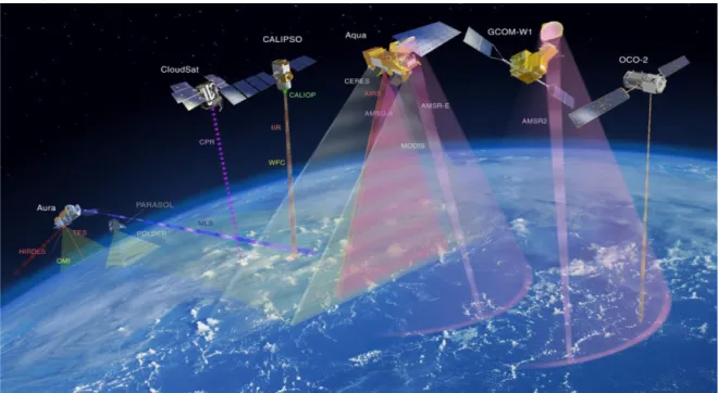
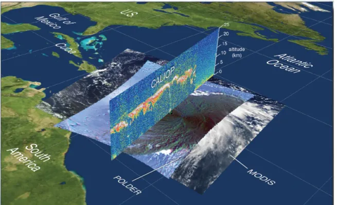
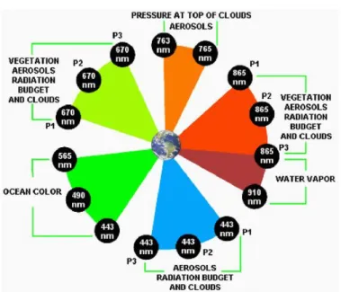
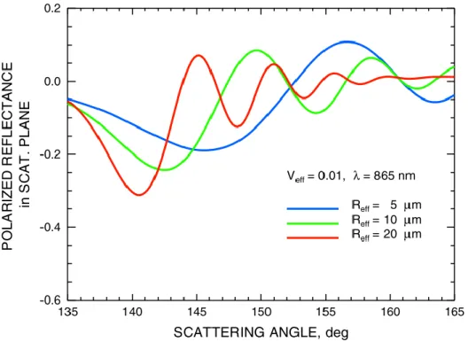
(13) Thèse de Christian Matar, Université de Lille, 2019. List of Figures. Figure 0-1: Distribution of different clouds types in three atmosphere levels: low, middle and high (Ahrens, 2015). ________________________________________________________________ 2 Figure 0-2: Qualitative radiative effect of clouds according to their altitude.. ______________________ 3. Figure I-1: Geometry of illumination and observation: θs and θv are the solar and view zenith angle, and φs and φv the solar and view azimuth angles.. _____________________________________ 14. Figure I-2: Representation of the international Afternoon Constellation (A-Train). Active instruments (CALIOP, CPR) are indicated with dashed lines. This illustration color-codes instrument swaths based on observed wavelength ranges. Microwaves (observed by both AMSR instruments, AMSU-A, CPR, MLS) are represented as red-purple to deep purple colors; yellow represents solar wavelengths (OMI, OCO-2, POLDER); gray represents solar and infrared wavelengths (MODIS, CERES); and red represents other infrared wavelengths (IIR, AIRS, TES, HIRDLS). Note that PARASOL ceased operation in December 2013. Source: NASA (https://atrain.gsfc.nasa.gov/historical_graphics.php). _______________________________________________________________ 22 Figure I-3: An image of Hurricane Bill as seen from the MODIS instrument (flying on Aqua) with cloud heights from the CALIOP lidar (on CALIPSO) on August 19, 2009. Superimposed over the MODIS image is the polarized reflected sunlight observed by POLDER (on PARASOL). Source: NASA. ___. 23. Figure I-4: Spectral and polarization channels of POLDER-2 with their mission purposes (from Bermudo et al., 2017). POLDER/PARASOL had one more channel at 1020 nm to compare with the measurements of CALIOP/CALIPSO.. _______________________________________________ 24. Figure I-5: 3MI multi-channel and multi-polarization concept exploiting two optical systems and a single rotating filter wheel (source: Eumetsat). __________________________________________. 27. Figure I-6: Theoretical relationships between the reflectance at 0.75 and 2.16 μm for various values of optical depth (vertical, dashed lines) and effective radius (solid lines) for a particular solar geometry that match aircraft data obtained during a field campaign conducted in July 1987 (From Nakajima and King, 1990).. ______________________________________________________ 29. Figure I-7: Sensitivity of polarized reflectance in the cloud bow angular range (scattering angles between 135º and 170º) to the effective radius cloud droplet size distribution (from Alexandrov et al., 2012). 31. Figure I-8: Relationship between radiance and cloud optical thickness. In a limited resolution, the average radiance R1,2 of two radiances R1 and R2 lead to a retrieved optical thickness COT’ smaller than the. vii © 2019 Tous droits réservés.. lilliad.univ-lille.fr.

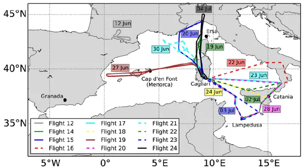
(14) Thèse de Christian Matar, Université de Lille, 2019. List of Figures. average optical thickness of the pixel COT 1,2 obtained if R1 and R2 are known (adapted from Zinner and Mayer, 2006). ___________________________________________________. 32. Figure I-9: Schematic representation of the COT retrieval errors due to the simplified 1D cloud model. Towards small scales, the Independent Pixel Approximation (IPA) increases because the cloud columns are not independent from each other. Towards large scales, the error increases due to the sub-pixel heterogeneity. This figure is adapted from a presentation by Warren Wiscombe based on the study of Davis et al. (1997).. ________________________________________________ 33. Figure I-10: Schematic representation of a triangle shape cloud vertical profile of Reff with the different depths of penetration of the polarized radiance (Rpol) and the total radiances at 3.7, 2.2 and 1.6 μm. __ 35. Figure II-1: Mechanical scheme of OSIRIS (from Auriol et al., 2008). _________________________. 38. Figure II-2: Spectral wavelengths of VIS-NIR (left) and SWIR (right) optical matrices of OSIRIS. The dashed line corresponds to a typical atmospheric transmittance. The red colored channels are used in this study (865, 1020, 1240, 1620 and 2200 nm).. _________________________________ 39. Figure II-3: Arrangement of the three analyzers P0, P1 and P2 in respect to the electrical field E.. _______ 40. Figure II-4: Overview of the different F-20 flight trajectories performed during the SOP-1a campaign of the CHARMEX/ADRIMED project (Mallet et al., 2016) ____________________________ Figure II-5: Overview of the different F-20 flight trajectories performed during the CALIOSIRIS.. 43. ______ 45. Figure II-6: In-lab image of OSIRIS at 865 nm with a light source on the left (long exposure time).. _____ 49. Figure II-7: In-lab experiment with OSIRIS at 865 nm with a light source on the left: the radiances captured after four filters FULL, P1, P2 and P3. The red rectangle on the FULL image represents the zone A used in the calculation of Rlab. ______________________________________________. 50. Figure II-8: Over ocean measurement of the campaign CALIOSIRIS, flight of 24 October 2014, for the OSIRIS filter P3 (865 nm) (left). The picture on the right is the same as the one to the left but with more contrast to show the thin circles of stray light type 2. ____________________________. 51. Figure II-9: Stray light type 2 present in the airborne measurement (same flight as in Figure II-8) for the OSIRIS filters: FULL, P1, P2 and P3 at 865 nm.. ____________________________________ 52. Figure II-10: The relative difference between the polarized radiance of the airborne measurement before and after the removal of the stray light type 2. _______________________________________. 53. Figure II-11: Invalidating and filling the defective pixels: (a) map of the invalidated defective pixels in the airborne campaign CHARMEX, (b) radiance at 1240 nm of a cloudy scene in 30 June 2013 (CHARMEX campaign). (c) is the same as (b) but after correction of the invalidated dead and defective pixels.. ____________________________________________________ 54. viii © 2019 Tous droits réservés.. lilliad.univ-lille.fr.

(15) Thèse de Christian Matar, Université de Lille, 2019. List of Figures. Figure II-12: (a) and (b) two successive images taken by OSIRIS over a cloudy scene in CALIOSIRIS2 on 24 October 2014. (c) and (d) are the same images as (a) and (b) but divided by the average image. The black arrow in (a) represents the direction of the airplane. _________________________. 56. Figure II-13: Average of 14 successive images of OSIRIS around the images shown in Figure II-12 (a) and (b).. _______________________________________________________________ 57 Figure II-14: Matrices of RMSE (a) and SSIM (b) for all the possible translations between the images shown in Figure II-12 (a) and (b). _______________________________________________. 58. Figure III-1: CHARMEX case study on the 30 June 2013 at 13:40 (local time): (a) Airplane trajectories during this day, (b) Quicklook provided by the LIDAR-LNG close to the observed scene. (c) OSIRIS true color RGB composite, obtained from the total radiances at channels 490, 670 and 865 nm. (d) OSIRIS true color RGB composite, obtained from the polarized radiances at channels 490, 670 and 865 nm.. _________________________________________________________ 68. Figure III-2: Same as Figure III-1 but for the case study CALIOSIRIS on 24 October 2014 at 11:02 (local time).. _______________________________________________________________ 69 Figure III-3: Total radiances (a, c and e) and absolute value of polarized radiances (b, d and f) as a function of the scattering angle for 490, 670 and 865 nm for different COT (1, 2, 4, 8, 16 and 32) with a constant Reff = 10 μm, veff = 0.02, altitude = 5 km, ocean wind speed = 8 m/s and θs= 60°. Brown color curve corresponds to the superposition of several colors in those graphs.. ___________________. 72. Figure III-4: Total radiances as a function of the scattering angle for the wavelengths 1020 (a), 1240 (b), 1620 (c) and 2200 nm (d) for different COT (1, 2, 4, 8, 16 and 32) with a constant Reff = 10 μm, veff = 0.02, altitude = 5 km, ocean wind speed = 8 m/s and θs= 60°. __________________________. 74. Figure III-5: Total radiances (a, c and e) and absolute value of polarized radiances (b, d and f) as a function of the scattering angle for 490, 670 and 865 nm for different R eff (5, 10, 15, 20, 25 and 30) with a constant COT = 10, veff = 0.02, altitude = 5 km, ocean wind speed = 8m/s and θs = 60°. The inset plots in b, d and f correspond to the absolute value of polarized radiances with variable R eff and a constant COT = 3. ___________________________________________________. 76. Figure III-6: Total radiances as a function of the scattering angle for the wavelengths 1020 (a), 1240 (b), 1620 (c) and 2200 nm (d) for different Reff (5, 10, 15, 20, 25 and 30 μm) with a constant COT = 10, veff = 0.02, altitude = 5 km, ocean wind speed = 8 m/s and θs = 60°. The inset plots correspond to the total radiances with variable Reff and a constant COT = 3. _________________________. 77. Figure III-7: Number of available directions (n) for each pixel in the visible matrix for the cases CALIOSIRIS (a) and CHARMEX (b). _______________________________________________. 79. Figure III-8: Retrieval of COT for CALIOSIRIS using mono-directional total radiance at 865 nm: (a) total radiance measured at 865 nm by OSIRIS, (b) retrieved COT, (c) simulated total radiance at 865 nm. ix © 2019 Tous droits réservés.. lilliad.univ-lille.fr.

(16) Thèse de Christian Matar, Université de Lille, 2019. List of Figures. using the COT retrieved, (d) uncertainties of the retrieved COT (Equation III-13), (e) relative difference between the measured and the simulated total radiance, and (f) cost function of the retrieval. _________________________________________________________. 80. Figure III-9: Total radiance at 865 nm as a function of COT: the grey shades represent the uncertainty on the COT attributed to 5% uncertainties in the radiances at θs=59.7º, θv=70º and φ=90º resulting in Θ=100º. Horizontal dashed red lines represent +/- 5% errors on radiances represented by the green dots. ____________________________________________________________ Figure III-10: Same as Figure III-9 but for the case study of CHARMEX.. 82. ______________________ 84. Figure III-11: Total radiance at 865 nm as a function of COT at the same viewing angle θv=70º and azimuthal angle φ=90º but with different solar zenith angles (sza): blue corresponds to sza=30º (CHARMEX) and green corresponds to sza=60º (CALIOSIRIS).. _____________________________ 85. Figure III-12: POLDER-like retrieval of COT using multi-angular radiance at 865 nm for CALIOSIRIS: (a) Field of COT retrieved and (b) corresponding uncertainties. (c) and (d) are the same as (a) and (b) respectively for CHARMEX. Arrows in (a) are used to identify two pixels that will be used later in a study on the pixel scale. ______________________________________________. 86. Figure III-13: POLDER-like retrieval representation for two pixels viewed under 8 directions: total radiance at 865 nm (left Y-axis) and COT (right Y-axis) as a function of the scattering angles, the pixels are from CALIOSIRIS at line 116 column 50 (a) and line 116 column 200 (b) of the CCD matrix. Blue arrows represent the scattering angle corresponding to the central image. _______________. 89. Figure III-14: OSIRIS_8 retrieval of COT using multi-angular radiance at 865 nm for CALIOSIRIS: (a) Field of COT retrieved and (b) corresponding uncertainties with the (c) normalized cost function and (d) convergence test.. ___________________________________________________ 90. Figure III-15: Same as Figure III-14 but for CHARMEX.. _________________________________ 92. Figure III-16: Comparison of retrieved COT using the POLDER-like and OSIRIS_8 methods for CHARMEX: (a) normalized frequency distribution of COT retrieved by both methods with an inset showing their angular relative difference over the whole field. Dashed curves represent the fitting frequency distribution functions for each method characterized by the mean μ and the standard deviation σ. (b) Scatter plot of retrieved COT by both methods; the colors represent the magnitude of the angular relative variance of mono-directional COTs used in the POLDER-like method (shown in the inset).. _______________________________________________________________ 94 Figure III-17: Same as Figure III-16 but for CALIOSIRIS.. ________________________________ 95. Figure III-18: OSIRIS_8 retrieval for the same two pixels of Figure III-13 viewed under 8 directions: total radiance at 865 nm (left Y-axis) and COT (right Y-axis) as a function of the scattering angles.. 97. x © 2019 Tous droits réservés.. lilliad.univ-lille.fr.

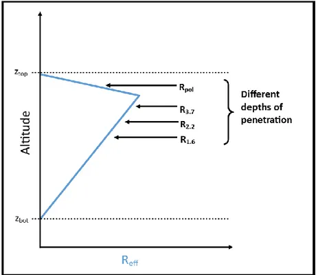
(17) Thèse de Christian Matar, Université de Lille, 2019. List of Figures. Figure III-19: Retrieval of COT and Reff for CALIOSIRIS using multi-angular total and polarized radiance at 865 nm: (a) total radiance measured by the 865 nm channel for the central image (b) polarized radiance measured by the 865 nm channel for the central image (c) retrieved COT, (d) retrieved R eff, (e) uncertainties on retrieved COT, (f) uncertainties on retrieved Reff, (g) normalized cost function and (h) convergence test.. _________________________________________________ 99. Figure III-20: Number of available directions for each pixel (n) in the NIR-SWIR matrix of the CALIOSIRIS (a) and CHARMEX (b) cases.. ____________________________________________ 101. Figure III-21: Diagram of radiances at 1020 and 2200 nm for various values of optical depth (vertical blue dashed lines) and effective radius (solid blue lines) for a solar zenith angle of 30° and a view zenith and azimuth angle equal to 50° and 20° respectively (scattering angle Θ=101°). The red diagram is the same as the blue but when 865 nm is used instead of 1020 nm.. ____________________ 103. Figure III-22: MODIS-like retrieval of COT and Reff for CHARMEX using mono-angular total radiances at 1020 and 2200 nm: (a) total radiance measured by the 1020 nm channel (b) total radiance measured by the 2200 nm channel (c) retrieved COT, (d) retrieved R eff, (e) uncertainties on retrieved COT, (f) uncertainties on retrieved Reff (g) normalized cost function and (h) convergence test. ______. 104. Figure III-23: OSIRIS_10-22 retrieval of COT and Reff for CHARMEX using multi-angular total radiances at 1020 and 2200 nm: (a) retrieved COT, (b) retrieved R eff, (c) uncertainties on retrieved COT, (d) uncertainties on retrieved Reff and (e) normalized cost function and (f) convergence test.. ___ 106. Figure III-24: Normalized frequency distribution retrieved COT (a) and Reff (b) using the MODIS-like and OSIRIS_10-22 methods for CHARMEX.. __________________________________ 108. Figure III-25: Scatter plot of retrieved COT using OSIRIS_10 and OSIRIS_10-22, the colors represent the values of Reff retrieved using OSIRIS_10-22. ____________________________________. 110. Figure III-26: (c) Normalized frequency distribution of radiances measured by the 865 nm (a) and the 1020 nm (b) channels in CHARMEX. ___________________________________________. 111. Figure III-27: OSIRIS_10-16 retrieval of COT and Reff for CHARMEX using total multi-angular radiances at 1020 and 1620 nm: (a) total radiance measured by the 1020 nm channel (b) total radiance measured by the 1620 nm channel (c) retrieved COT, (d) retrieved Reff, (e) uncertainties on retrieved COT, (f) uncertainties on retrieved Reff, (g) normalized cost function and (h) convergence test.. _____ 113. Figure III-28: Comparison of retrieved Reff using the OSIRIS_10-22 and OSIRIS_10-16 methods for CHARMEX: (a) normalized frequency distribution of Reff retrieved by both, and (b) scatter plot of retrieved Reff by both methods, with a color scale representing the normalized frequency. ___ 115. Figure III-29: Diagram of radiances at 1020 and 1620 nm for various values of optical depth (vertical dashed lines) and effective radius (solid lines) for a solar zenith angle of 30° and a view zenith and azimuth angle equal to 50° and 20° respectively (scattering angle Θ=101°). __________________. 116. xi © 2019 Tous droits réservés.. lilliad.univ-lille.fr.

(18) Thèse de Christian Matar, Université de Lille, 2019. List of Figures. Figure III-30: MODIS-like retrieval of COT and Reff for CALIOSIRIS using mono-angular total radiances at 1240 and 2200 nm: (a) total radiance measured by the 1240 nm channel (b) total radiance measured by the 2200 nm channel (c) retrieved COT, (d) retrieved Reff, (e) uncertainties on retrieved COT, (f) uncertainties on retrieved Reff (g) normalized cost function and (h) convergence test. We not that (d) and (f) have a different color scale maximum.. _______________________________ 117. Figure III-31: Diagram of radiances at 1240 and 2200 nm for various values of optical depth (vertical dashed lines) and effective radius (solid lines) for a solar zenith angle of 60° and a view zenith and azimuth angle equal to 40° and 70° respectively (scattering angle Θ=101°). __________________. 118. Figure III-32: OSIRIS_12-22 retrieval of COT and Reff for CHARMEX using multi-angular total radiances at 1240 and 2200 nm: (a) retrieved COT, (b) retrieved R eff, (c) uncertainties on retrieved COT, (d) uncertainties on retrieved Reff, (e) normalized cost function and (f) convergence test. ______. 120. Figure III-33: Comparison of retrieved Reff using the OSIRIS_12-22 and OSIRIS_12-16 methods for CALIOSIRIS: (a) normalized frequency distribution of retrieved Reff by both methods and (b) scatter plot of retrieved Reff by both methods; the colors represent the magnitude of retrieved COT with OSIRIS_12-22.____________________________________________________. 121. Figure IV-1: The uncertainties on COT (left) and Reff (right) originating from the measurement errors for different couples of COT and Reff. Uncertainties are represented by the relative standard deviation (RSD). Values of Reff vary between 2 and 29 µm and values of COT vary from 0.1 to 100 on a logarithmic axis. ___________________________________________________________. 129. Figure IV-2: Altitude of the backscattering maximum of the LIDAR-LNG signal in function of time for the case of CALIOSIRIS, the blue vertical lines limit the studied scene.. ____________________ 131. Figure IV-3: Averaged polarized radiances measured by OSIRIS for a transect in the middle of the central image of CALIOSIRIS (in red) and the simulated polarized radiance with an effective radius of water droplets equal to 0.02 (in blue), as a function of the scattering angles. The positions of the supernumerary bows coincide for a value of veff equal to 0.02. _____________________. 132. Figure IV-4: Same as Figure IV-1 but for the uncertainties on the retrieved COT and Reff originating from the ancillary parameters errors: altitude (a and b), the effective variance of water droplets (c and d) and the surface wind speed (e and f).. ________________________________________ 134. Figure IV-5: The heterogeneous vertical profile of effective radius (black line) and extinction coefficient (blue line) used to assess uncertainties due to the assumption used for the vertical profile. The homogeneous vertical profiles are shown in dashed lines. ________________________. 139. Figure IV-6: Same as Figure IV-1 but for the uncertainties on the retrieved COT and Reff originating from the homogenous vertical profile assumed in the forward model.. ______________________ 140. xii © 2019 Tous droits réservés.. lilliad.univ-lille.fr.

(19) Thèse de Christian Matar, Université de Lille, 2019. List of Figures. Figure IV-7: COT (a) and Reff (b) retrieved using OSIRIS_12-22 for the case study CALIOSIRIS_2 in 30 June 2014 at 11:02:18.. __________________________________________________ 142. Figure IV-8: Uncertainties (%) on COT (left) and Reff (right) originating from the measurements error for the case study of CALIOSIRIS ____________________________________________. 142. Figure IV-9: The uncertainties (%) on COT and Reff originating from the ancillary parameter errors: altitude (a and b), the effective variance of water droplets (c and d) and the surface wind speed (e and f).. 144. Figure IV-10: The uncertainties (%) on COT and Reff originating from the assumptions in the forward, for not taking into account: the heterogeneous vertical profile (a and b) and the 3D radiative behavior of radiations (c and d). _________________________________________________. 145. Figure IV-11: The simulated 1D (a) and 3D (b) radiances at 1240 nm using the retrieved COT and Reff presented in Figure IV-7 for the central image. (c) and (d) are the same as (a) and (b) but for 2200 nm. _. 147. Figure IV-12: Histograms of the relative difference between the radiances computed in 1D and 3D at 1240 nm for the central image. Each histogram corresponds to a domain of COT.. ______________ 148. Figure IV-13: Uncertainties on the retrieved COT (a) and Reff (b) originating from the 3D radiative model as a function of the absolute difference |R1D-R3D| at each pixel averaged for all the directions available at 1240 nm (a) and 2200 nm (b). THE horizontal LINE. _________________________ 149. Figure IV-14: Histograms of the mean uncertainties on the retrieved COT and Reff in CALIOSIRIS_2: RSD COT (green bars) and RSD Reff (blue bars), for the different sources of error. Red error bars represent the standard deviation of the uncertainties.. ____________________________________ 151. xiii © 2019 Tous droits réservés.. lilliad.univ-lille.fr.

(20) Thèse de Christian Matar, Université de Lille, 2019. List of Tables. Table I-1: Analytical equations and typical values of number concentration, average volume, surface and mass of water droplets.. _____________________________________________________ 9. Table I-2: Spectral bands used on MODIS in cloud products: their central wavelength, their ground resolution and their principal purposes ______________________________________________. 26. Table II-1: Summary of CHARMEX/ADRIMED flights details with some notes. The - and + in the interest column refer to negative and positive interest respectively. A positive (+) interest indicates the possibility of choosing a case study from the corresponding flight.. ____________________ 44. Table II-2: Summary of CALIOSIRIS flights. The - and + in the interest column refer to negative and positive interest respectively. A positive interest indicates the possibility of choosing a case study from the corresponding flight.. __________________________________________________ 46. Table III-1: Methods used with the visible channels of OSIRIS to retrieve COT and Reff, with the corresponding measurement vector 𝐲 and state vector 𝐱. _____________________________________. 78. Table III-2: Comparison of the mean retrieved COT (in bold font) and its mean uncertainty (between the parentheses) using the mono-directional and the POLDER-like methods for CALIOSIRIS and CHARMEX.. _______________________________________________________ 87. Table III-3: Methods used with the NIR-SWIR channels of OSIRIS to retrieve COT and Reff, with the corresponding measurement vector 𝐲 and state vector 𝐱. __________________________. 101. Table III-4: The mean retrieved COT and Reff (in bold font) and their mean uncertainties (between the parentheses) using the different methods used in this chapter for CALIOSIRIS and CHARMEX. “*” is used to represent a parameter not retrieved and set to a constant value in the retrieval. _____. 123. xiv © 2019 Tous droits réservés.. lilliad.univ-lille.fr.

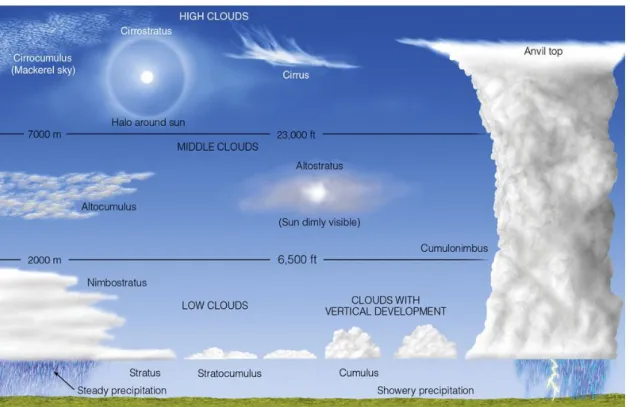
(21) Thèse de Christian Matar, Université de Lille, 2019. Introduction. “The beginning is the most important part of the work” Plato ~ It dates back to 1896 when the Swedish scientist Svante Arrhenius was the first to suggest that human emissions might warm the planet and create the problematic of the century, “the climate change”. Many studies addressed this issue from different perspectives, it made us sure about some things like the fact that we are heading to a warmer planet but there is still a lot that we do not understand. The Fifth Assessment Report by the International Panel on Climate Change (IPCC - Boucher et al., 2013) states that “Human influence on the climate system is clear, and recent anthropogenic emissions of greenhouse gases are the highest in history” and that “Warming of the climate system is unequivocal, and since the 1950s, many of the observed changes are unprecedented over decades to millennia”. However, large inconsistencies exist in the prediction of climate warming at the end of the century. The disagreement in the warming predictions originates from the uncertainties associated with radiative forcing and feedback estimations for the main drivers of climate change, among which clouds are a major contributor (Arakawa, 1975, 2004; Bony et al., 2006; Caldwell et al., 2018; Cess et al., 1990; Charney and DeVore, 1979; Randall et al., 2003). That being said, clouds are a fundamental aspect of humanity, not only by providing fresh water supplies, but also by regulating the temperature of the planet Earth. However, the quantification of this role is not an easy task. The clouds effect on the radiation that enters and leaves the atmosphere has to be addressed by observing their distributions, variabilities and properties over time. As per the World Meteorological Organization (WMO), the clouds are divided into ten types according to the altitude of their base and their approximate appearance. They are distributed in three altitude levels (Figure 0-1): low-level clouds (Cumulus, Stratus and Stratocumulus and Nimbostratus), middle-level clouds (Altocumulus and Altostratus), high-level clouds (Cirrus, Cirrocumulus and Cirrostratus) and the vertically extended cloud (Cumulonimbus).. 1 © 2019 Tous droits réservés.. lilliad.univ-lille.fr.

(22) Thèse de Christian Matar, Université de Lille, 2019. Introduction. Figure 0-1: Distribution of different clouds types in three atmosphere levels: low, middle and high (Ahrens, 2015) Depending on their altitude, clouds have different impacts on the Earth radiative budget. Low thick clouds block out the sun reflecting about 50 w/m2 (20%) of the incoming solar radiation. They have an important albedo effect and contribute mainly to the cooling of the atmosphere. High wispy clouds like the cirrus are transparent for shortwave radiations and have thus a weak albedo effect. At the same time, they have a strong greenhouse effect since they absorb the longwave radiation emitted by the Earth surface and re-emit it towards the ground and space. This process traps about 30 w/m2 of the Earth infrared radiation and heats up the atmosphere. The net radiative budget of the cloud is then around -20 w/m2. However, the difficulty arises in the estimation of cloud feedback in the future and whether it is going to amplify or limit the climate warming.. 2 © 2019 Tous droits réservés.. lilliad.univ-lille.fr.

(23) Thèse de Christian Matar, Université de Lille, 2019. Introduction. Figure 0-2: Qualitative radiative effect of clouds according to their altitude.. Indeed, clouds are not alone in the climate system. We cannot overlook the cloud feedback influenced by other climate variables, such as the increase of surface temperature and water vapor concentrations. High clouds are expected to rise in altitude where the lower temperature results in less re-emission of long-wave radiation increasing the cloud greenhouse effects. Low clouds seem to be moving from the tropics toward the poles, contributing in the planet warming by being less effective in blocking the intense tropical Sun radiation (Marvel et al., 2015; Norris et al., 2016). Subtle changes of cloud properties can occur due to the climate warming and also to anthropogenic emissions of small aerosol particles, which act as cloud condensation or ice nuclei. Even small variations of cloud cover and properties can have profound consequences on the Earth’s climate. This adds more to the complexity of clouds study. They have to be characterized on the microscopic scale of water droplets or ice crystals forming the clouds, and on the larger scale since they cover two-thirds of the earth's surface (Rossow and Schiffer, 1999). Fortunately, we do have different types of clouds observation techniques covering different scales. They improve our overall representation of clouds and their properties, validate the results of climate models and characterize the cloud-aerosol interactions. Each instrument has been designed for specific applications and may have particular limitations:. 3 © 2019 Tous droits réservés.. lilliad.univ-lille.fr.

(24) Thèse de Christian Matar, Université de Lille, 2019. Introduction. range, resolution, continuity, coverage and precision. The Ground-based observations provide continuous data but are spatially limited, as they do not allow a global vision of the planet and lack the coverage over the ocean or Polar Regions. On the other hand, airborne observations are useful for case studies on a regional scale, and for testing and validating the spatial instruments. They are localized in space and time but the low altitude flights provide high spatial resolution data, allowing an enhanced representation of the cloud variabilities. In situ airborne measurements exist also; they add more information on the properties of particles in a case study. The progress of artificial satellites technology in the 20th century allowed remote sensing on a global scale: the satellite observations. The satellites of different space missions, starting from TIROS (Television Infrared Observation Satellites) in 1960, to the Geostationary Operational Environmental Satellite (GOES), the Polar-orbiting Operational Environmental Satellite (POES), the Afternoon constellation (A-train) and many other systems, are the main provider of Earth observations. These space missions carried passive instruments that rely on the modification of solar or thermal radiation by the atmosphere (e.g. Moderate Resolution Imaging Spectroradiometer (MODIS), POLarization and Directionality of the Earth's Reflectances (POLDER)...). In addition, since the A-train mission, satellites started to carry active instruments that use their own source of radiation and provide a vertical profile of aerosols and clouds (e.g. Cloud-Aerosol Lidar with Orthogonal Polarization (CALIOP), Cloud Profiling Radar (CPR)). The cloud properties are retrieved using the information carried by the measurements of the reflected (or transmitted) radiations by the clouds. Two main optical cloud properties are generally retrieved: the cloud optical thickness (COT) and the effective radius of the water/ice particles forming the cloud (Reff). These optical properties, along with the cloud altitude, allow to characterize the clouds at a global scale and help to determine the radiative impacts of clouds along with their cooling and warming effects (Lohmann and Feichter, 2005; Platnick et al., 2003; Twomey, 1991). Three passive remote sensing methods are commonly used in the retrievals of these optical properties. The infrared split-window technique (Giraud et al., 1997; Inoue, 1985; Parol et al., 1991) uses infrared measurements and is more suitable for optically thin ice clouds (Garnier et al., 2012). The bispectral method (Nakajima and King, 1990) which uses visible and shortwave infrared wavelength, is more suitable for optically thick clouds, often water cloud. It is currently used in a lot of operational algorithms and in. 4 © 2019 Tous droits réservés.. lilliad.univ-lille.fr.

(25) Thèse de Christian Matar, Université de Lille, 2019. Introduction. particular for MODIS (Platnick et al., 2003). It is also possible to use a combination of multiangular total and polarized measurements in the visible range, such as POLDER measurements (Deschamps et al., 1994), in order to retrieve COT and Reff (Bréon and Goloub, 1998; Buriez et al., 1997). In the operational algorithms, the retrieval of COT and Reff is achieved through precomputed Look-Up Tables (LUT). These LUT are a multi-dimensional array, with each dimension containing modeled radiances for a combination of properties to be retrieved, at different wavelengths, surfaces types, cloud phase and geometry of observation and illumination. Knowing the radiances observed, the parameter(s) to be retrieved could be found by searching and interpolating the values in the LUT. This method can be used to process large database automatically. Its disadvantage is that a modification of the particle model or any other model parameter requires re-generating all these pre-calculated tables. Adding to that, for simplicity and computational time reasons, the computation of radiances is done under the hypothesis of a single homogeneous cloud layer between two parallel and infinite planes, which implies that the cloud columns are considered independent from each other. This allows the retrieval of several parameters (phase, droplets or crystals size, optical thickness...) but can lead to large uncertainties that add to the uncertainties originating from the measurements. For example, there is a disagreement in the retrievals of the cloud droplets effective radius according to the information used in these retrievals (Bréon and Doutriaux-Boucher, 2005; Platnick, 2000; Zhang and Platnick, 2011). These inconsistencies appear to be mainly due to the strong hypothesis of horizontally and vertically homogeneous cloud. More identified errors are related to the subpixel variability of cloud properties (Cahalan et al., 1994), illumination and shadowing effects of solar radiation (Várnai and Marshak, 2002) or horizontal transport between cloud columns (Marshak et al., 1998). Therefore, the uncertainties on the retrieved properties, originating from the simulations and the observations have to be assessed. Indeed, the uncertainties estimates are one of the recommendations of the International Cloud Working Group (ICWG)*.. * http://www.icare.univ-lille1.fr/highlights_data/images/workshop_2018_first_announcement/Announcement_I_ICWG-2_Workshop_2018.pdf. 5 © 2019 Tous droits réservés.. lilliad.univ-lille.fr.

(26) Thèse de Christian Matar, Université de Lille, 2019. Introduction. The aim of the science community is to use multiple types of observations and retrieval methods to complete the gaps in our knowledge about the role of clouds in meteorological forecast and climate change. That is why more missions are planned in the future, like Earthcare and EPS-SG in 2022. One of the instruments that will be carried in those space missions is 3MI (Multi-viewing Multi-channel Multi-polarization Imaging), planned to be launched on MetOp-SG (2022). It has the multi-angular and polarized measurements capabilities of its ancestor POLDER extended to the shortwave infrared. In order to prepare for the future cloud retrieval algorithms of 3MI, during this thesis, we work on the measurements of OSIRIS the airborne prototype of 3MI. OSIRIS was developed in the Laboratoire d’Optique Atmosphérique (Lille, France). It can measure the degree of linear polarization from 440 to 2200 nm. It is has been used onboard the French research aircraft, Falcon-20, during several airborne campaigns: CHARMEX/ADRIMED (Mallet et al., 2016), CALIOSIRIS and AEROCLO-sA (Formenti et al., 2018). Besides the possibility to have dedicated objectives over geographical areas campaigns, the advantage of these airborne measurements lies in the high spatial resolution (a few tens of meters) compared to spatial measurements, which allow a better characterization of the clouds. OSIRIS is currently in test phase, we apply several pre-retrieval processes to improve the ability of using its measurements. We couple the multi-angular visible and shortwave infrared measurements of OSIRIS with a statistical inversion method in order to obtain a flexible retrieval process of COT and Reff. The exploitation of the additional information on the cloud provided by these versatile measurements implies the use of a more complex retrieval method of clouds properties. The algorithm is based on the optimal estimation method (Rodgers, 1976, 2000). It is a more sophisticated inversion method compared the LUT and has been widely used for applications in cloud remote sensing (Cooper et al., 2003; Poulsen et al., 2012; Sourdeval et al., 2013; Wang et al., 2016). In this method, the Bayesian conditional probability together with a variational iteration method allows the convergence to the physical model that best fit the measurements. Therefore, it introduces probability distribution of solutions where the retrieved parameter being the most probable, with an ability to extract uncertainties on the retrieved parameters. Our aim is to: 1) Enhance the state of OSIRIS measurements by characterizing potential artifacts and developing the techniques needed to exploit its measurements at best.. 6 © 2019 Tous droits réservés.. lilliad.univ-lille.fr.

(27) Thèse de Christian Matar, Université de Lille, 2019. Introduction. 2) Retrieve COT and Reff by a new approach that benefits from the versatility of OSIRIS/3MI measurements and compare it with the POLDER and MODIS-like methods. 3) Build the mathematical framework needed to study the uncertainties on the retrieved cloud properties that separate the contributions of different sources of uncertainties, and for the first time, quantify the magnitude of the simplified 1D cloud model used on real cloud reflected measurements. In the first chapter, we present a background on the physical theories that allow us to describe the atmosphere-radiation interaction, the core of remote sensing techniques. Likewise, we discuss the insights of different instrumentations and approaches used to study the clouds, while focusing on the A-train constellation mission and the three instruments related to our work: POLDER, MODIS and 3MI, along with a more detailed outline of the two retrieval methods used with POLDER and MODIS. In the second chapter, we describe the multi-angular, multi-spectral and polarized characteristics of the instrument OSIRIS and basic details of the airborne campaigns CHARMEX and CALIOSIRIS. We discuss also several operations that needed to be addressed before the retrieval process including the stray light corrections and tracking of the cloud scenes that permits to obtain the multi-angular measurements. In the third chapter, we report a description of the optimal estimation method used in the retrieval algorithms developed in this thesis as well as the forward model constructed to simulate the radiations scattered by the clouds and captured by OSIRIS. We present also the sensitivity of OSIRIS channels on the cloud optical thickness and the effective radius of water cloud droplets. Then we show the results of different techniques of retrievals for two case studies: a mid-level thin cloud and a low-level thick cloud. The retrieved values are compared with the results obtained by the classical retrieval algorithms of MODIS and POLDER. Since the optimal estimation method allows the quantifying of uncertainties on the retrieved parameters, in the fourth chapter, we assess the magnitude of different types of errors, such as the errors due to measurements noise, the errors linked to the fixed parameters in the simulations and the errors related to the unrealistic homogeneous cloud assumption. Finally, we will give the concluding remarks and the perspectives of this thesis.. 7 © 2019 Tous droits réservés.. lilliad.univ-lille.fr.

(28) Thèse de Christian Matar, Université de Lille, 2019. I Clouds and Atmospheric Radiations Clouds are composed of water droplets and ice crystals. They are visible through the scattering of light by these small particles. White or gray contrasted with a blue sky, the different color shades a cloud can have, are a vast indicator of the cloud-radiation interaction, which is a major part of the atmosphere-radiation interaction. Cloud studies can thus be done remotely. It requires accurate simulations of the radiation propagating the atmosphere and interacting with the clouds, coupled with accurate observations of the results of these interactions. In this chapter, we will review the fundamentals of this coupling system, from the interactions to the measurements.. I.1 The Cloud-Radiation Interaction To study the propagation of radiation in the clouds, we have to look first into the interaction between radiations and cloud components. This interaction is responsible for numerous phenomena such as absorption and scattering. The following sections are devoted to define the optical and radiative quantities related to this interaction.. I.1.1 Cloud microphysics Any volume of air defined by its temperature and water vapor is called an air mass. The hotter the air mass, the more it can be loaded with water vapor until it reaches a saturated concentration. When a saturated air mass is cooled under a threshold temperature (dew point), water vapor will condense and form droplets. It happens generally during an upward movement of air in the lowest atmosphere layer “the troposphere”, where the mean. 8 © 2019 Tous droits réservés.. lilliad.univ-lille.fr.

(29) Thèse de Christian Matar, Université de Lille, 2019. I.1 The Cloud-Radiation Interaction. temperature decreases with altitude. This process produces a liquid or ice water cloud depending on the temperature and available condensation nuclei (Koop et al., 2000). The particles then may grow by additional condensation or by coalescence during collision with other particles. When they become large enough, they fall in and out of the cloud as precipitation. In this thesis, we are interested in liquid clouds composed of water droplets. We introduce the microphysical properties that help to describe the vast number of cloud droplets within each cloud. Due to the spatial and temporal variability of the air physical properties and variabilities in the cloud condensation particles size, a constant dimension for all the particles cannot be assumed (Twomey, 1977). Thus, we consider that the distribution of droplet radius 𝑟 can be approached by a particle size distribution (PSD). The distribution can have any shape but generally, it is approximated by a gamma distribution (Deirmendjian, 1964), a log-normal distribution (Hansen and Travis, 1974) or any other analytical formulas that match values measured in various types of clouds (Hobbs, 1981). In this work, we use the log-normal distribution: 𝑛(𝑟) =. 1 √2𝜋𝜎𝑟. 𝑒. −. 𝑙𝑛2 (𝑟/𝑟𝑚 ) 𝜎2. Equation I-1. where 𝑟𝑚 is the mean radius of water droplets and 𝜎 2 is the distribution variance. Different parameters can then be defined using this distribution, e.g. the particle number concentration 𝑁, the average volume of water droplets < 𝑉 > , the average surface they occupy < 𝑆 > and their average mass < 𝑊 >. They are listed in Table I-1 along with their typical order of values. Table I-1: Analytical equations and typical values of number concentration, average volume, surface and mass of water droplets. Quantity. 𝑁. Analytical equation. ∫ 𝑛(𝑟)𝑑𝑟. Typical order of values. 100/cm3. ∞ 0. <𝑉>. <𝑆>. ∞ ∞ 4 𝜋 ∫ 𝑟 3 𝑛(𝑟)𝑑𝑟 4𝜋 ∫ 𝑟 2 𝑛(𝑟)𝑑𝑟 3 0 0. 10-16 m3. 10-12 m2. <𝑊>. 𝜌𝑤𝑎𝑡𝑒𝑟 < 𝑉 > 10-10 g. 9 © 2019 Tous droits réservés.. lilliad.univ-lille.fr.

(30) Thèse de Christian Matar, Université de Lille, 2019. Chapter I: Clouds and Atmospheric Radiations. Numbers indicated in the second line of Table I-1 are typical values. Even if water droplets show very small dimensions, their large numbers influence the extinction of light in the cloud and control significant aspects of the atmospheric processes. Moreover, though these quantities we can obtain more parameters that describe the cloud. Like the liquid water content (𝐿𝑊𝐶) expressed in kg/m3: ∞. 𝐿𝑊𝐶 = 𝜌𝑤𝑎𝑡𝑒𝑟 ∫ 0. 4 3 𝜋𝑟 𝑛(𝑟)𝑑𝑟 3. Equation I-2. The importance of this property is that it removes any dependency on the type of PSD, 𝑛(𝑟) used. Indeed, light extinction in a cloud having the same 𝐿𝑊𝐶 and particles size with different PSDs will be almost identical (Kokhanovsky, 2004). 𝐿𝑊𝐶 varies all over the cloud and, for non-precipitating clouds, has larger values at the cloud top (Feigelson, 1984). An integrated water content can be calculated using the geometrical thickness of the cloud, it is the liquid water path (𝐿𝑊𝑃) defined as: 𝑧𝑡𝑜𝑝. 𝐿𝑊𝑃 = ∫. 𝐿𝑊𝐶(𝑧)𝑑𝑧. Equation I-3. 𝑧𝑏𝑜𝑡. where 𝑧𝑡𝑜𝑝 and 𝑧𝑏𝑜𝑡 represent the cloud top and bottom altitudes. 𝐿𝑊𝑃 is usually given in g/m2 and, with the particle size, it links the 𝐿𝑊𝐶 with the reflected solar radiation by the cloud: the smaller the 𝐿𝑊𝑃, the less opaque the cloud.. I.1.2 Characteristics of radiation Now that we introduced the basic cloud microphysical properties, we must define the second element of the cloud-radiation interaction. In the atmosphere, radiations are streams of photons carrying the energy originating from the Sun, the Earth’s surface and the atmosphere itself. The amount of energy transported by these photons defines different types of radiation but the studies presented in this thesis are restricted to the domain of solar radiations. It covers the visible part of the solar spectrum between violet and red (0.4-0.7 μm), the infrared wavelengths from the Near InfraRed (NIR, 0.7-1.4 μm) and the Short-Wavelength Infrared (SWIR, 1.4-5 μm).. 10 © 2019 Tous droits réservés.. lilliad.univ-lille.fr.

(31) Thèse de Christian Matar, Université de Lille, 2019. I.1 The Cloud-Radiation Interaction. In addition to the description of light as photons streams, the dual nature of light allows its “wave” definition. In fact, the solar radiation field can be defined as a superposition of plane and monochromatic electromagnetic waves. Each of these transverse waves consists of an electric field and a magnetic field simultaneously oscillating and propagating at the speed of light. They are mutually perpendicular to each other and to the propagation direction. By convention, the geometrical orientation of the electric field defines the polarization of electromagnetic waves.. I.1.2.1 Stokes vector Due to the electromagnetic nature of radiation and the necessity to consider the polarization and scattering effects (that will be addressed in the following sections), radiations cannot be addressed in a scalar framework. The four-element Stokes vector provides a detailed mathematical description of the electromagnetic waves and their state of polarization (Chandrasekhar, 1950; Van de Hulst, 1957; Stokes, 1852): 𝐼 𝑄 𝑺=( ) 𝑈 𝑉. Equation I-4. - 𝐼 describes the total intensity of the radiation, - 𝑄 and 𝑈 correspond to the linear polarization state, - 𝑉 defines the circular polarization state. In case of purely monochromatic and coherent radiation, the wave is totally polarized and the Stokes parameters verify the relation: 𝐼2 = 𝑄2 + 𝑈 2 + 𝑉 2. Equation I-5. This is not the case for natural radiation. In fact, solar radiation reaching the top of the atmosphere is an equal mixture of polarizations; there is no dominant polarization direction and thus light is unpolarized (𝑄 = 𝑈 = 𝑉 = 0). However, with its interaction with the atmospheric components (molecules, stratospheric and tropospheric aerosols and clouds) and surfaces (vegetation, bare soil, snow, ice, water…), the radiation gradually becomes polarized. The relation between the Stokes parameters becomes:. 11 © 2019 Tous droits réservés.. lilliad.univ-lille.fr.

(32) Thèse de Christian Matar, Université de Lille, 2019. Chapter I: Clouds and Atmospheric Radiations 𝑄 2 + 𝑈 2 + 𝑉 2 = 𝐼𝑝2 ≤ 𝐼 2. Equation I-6. 𝐼 = 𝐼𝑛𝑎𝑡 + 𝐼𝑝. Equation I-7. with:. where 𝐼𝑛𝑎𝑡 and 𝐼𝑝 are respectively the natural (or unpolarized) and polarized components of radiation. It is also worth to mention that the circular polarization generated by the radiation interaction with the atmosphere is very weak (Kawata, 1978). Therefore, the fourth parameter 𝑉 can be neglected. The Stokes vector allows the computation of radiative quantities in the simulations needed for remote sensing application.. I.1.2.2 Radiative quantities In a remote sensing application, the propagation of radiation in the atmosphere ends when the radiation hits the surface of the detector. The knowledge of the measured radiation quantity is thus necessary. Its magnitude is related to the properties of the observed scene, but not solely. It also depends on many other parameters related to the instrument (e.g. the spectral response of its filters, the surface and orientation of the detector…) and are generally accounted for in the calibration phase of the instrument. In this section, we present the physical quantities useful for the description of radiation measured by passive remote sensing instruments, which are the main provider of measurements in our work.. Radiant flux The detectors of optical instruments are sensitive to the amount of light energy 𝜖𝑙 they receive during an observation period, the integration time (fixed by the electronics of the instrument). This energy is provided by photons of various wavelengths with different spectral energy 𝜖(𝜆), hence the role of filters that determine the instrument spectral sensitivity 𝑆(𝜆). Thereby, the energy an instrument receives during the integration time, with a sensitivity 𝑆(𝜆) between [λ1, λ2] is:. 12 © 2019 Tous droits réservés.. lilliad.univ-lille.fr.

(33) Thèse de Christian Matar, Université de Lille, 2019. I.1 The Cloud-Radiation Interaction 𝜆2. 𝜖𝑙 = ∫ 𝑆(𝜆)𝜖(𝜆)𝑑𝜆. Equation I-8. 𝜆1. The spectral energy 𝜖(𝜆) is expressed in joules per unit of wavelength, 𝑆(𝜆) is unitless and the energy 𝜖𝑙 is expressed in joules. We note that all the following quantities are defined in the interval [λ1, λ2] corresponding to the limit of the spectral filters. We can then define the radiant flux 𝜙 (in watts) representing the variation of energy a detector receives over a time interval 𝑑𝑡: 𝜙=. 𝑑𝜖𝑙 (𝑡) 𝑑𝑡. Equation I-9. Irradiance The amount of radiant flux reaching the detectors depends on the instantaneous field of view observed by the detector. To remove this dependency, it is necessary to introduce the irradiance, which is the radiant flux per surface unit 𝑑𝑠: 𝐸=. 𝑑𝜙 𝑑𝑠. Equation I-10. The irradiance characterizes the light power reaching a surface perpendicular to the light source per unit area. It is expressed in watts per surface unit (W/m2).. Radiance The irradiance also depends on the orientation of the detector with respect to the light direction. To obtain a unit independent of these characteristics, the radiance 𝑅 ∗ is defined. It is the flux reaching the instrument per unit area 𝑑𝑠 in a solid angle 𝑑Ω (sr), perpendicular to the surface of the detector: 𝑑2 𝜙 𝑅 = 𝑑𝑠𝑑Ω cos 𝜃𝑑 ∗. Equation I-11. where 𝜃𝑑 represents the angle between radiation and the normal to the surface of the detector (Figure I-1). The radiance is expressed in W.m-2.sr-1.. 13 © 2019 Tous droits réservés.. lilliad.univ-lille.fr.

(34) Thèse de Christian Matar, Université de Lille, 2019. Chapter I: Clouds and Atmospheric Radiations. The observed radiance depends on the geometry of illumination. In case of solar source, the incoming solar radiation is characterized by a solar zenith angle 𝜃𝑠 and azimuthal 𝜑𝑠 . The radiance depends also on the geometry of observation characterized by the view zenith angle 𝜃𝑣 (which is equal to 𝜃𝑑 ) and the view azimuth angle 𝜑𝑣 . Generally, we use the relative azimuth angle 𝜑𝑟 , which is the difference between the solar and observation azimuth angles, 𝜑𝑠 and 𝜑𝑣 (Figure I-1).. Figure I-1: Geometry of illumination and observation: 𝜃𝑠 and 𝜃𝑣 are the solar and view zenith angle, and 𝜑𝑠 and 𝜑𝑣 the solar and view azimuth angles.. Normalized radiance The quantity that is typically used in remote sensing is the normalized radiance 𝑅 (unitless) at the top of the atmosphere: 𝑅(𝜃𝑠 , 𝜃𝑣 , 𝜑𝑟 ) =. 𝜋𝑅 ∗ (𝜃𝑠 , 𝜃𝑣 , 𝜑𝑟 ) 𝐹0. Equation I-12. where 𝐹0 is the perpendicular solar irradiance incident on the Earth’s atmosphere. We can relate the measured radiance to the Stokes vector: - The total normalized radiance 𝑅 is proportional to the first Stokes parameter 𝐼. - The polarized normalized radiance 𝑅𝑝 is expressed according to the following equation:. 14 © 2019 Tous droits réservés.. lilliad.univ-lille.fr.

(35) Thèse de Christian Matar, Université de Lille, 2019. I.1 The Cloud-Radiation Interaction. 𝑅𝑝 ∝ √𝑄 2 + 𝑈 2 + 𝑉 2. Equation I-13. Hereafter we will use the normalized radiance 𝑅 that will be referred as “radiance”.. I.1.3 Basics of radiative transfer We briefly presented the general quantities used to define clouds and radiations. We devote the next subsections to introduce the interactions that may encounter the radiations while passing through the clouds on their way to reach the detector.. I.1.3.1 Extinction processes The propagation of electromagnetic radiation in the Earth’s atmosphere is governed by different types of interactions. They define the amount of radiant intensity lost and/or gained along the direction of traveling. The ability of any medium to interact with a photon is given by the photon mean free path. The denser the medium is, the more interactions a photon have and thus the smaller is the mean free path. In radiative transfer theory, the inverse of the mean free path is more commonly used. It is the extinction coefficient 𝜎𝑒𝑥𝑡 , expressed in a unit of m-1. We use it to indicate how the energy of light is attenuated along a distance of one meter. A small extinction coefficient means that the medium is relatively transparent to the beam while a large value points out that the beam is highly attenuated by the medium. Now considering the interaction of the solar radiation with the atmosphere, which is the case in our work, an incoming photon can either be absorbed or scattered by atmospheric molecules. Thus, a beam of light traversing the atmosphere may lose energy through these two processes, and the extinction coefficient is the sum of these two contributions: 𝜎𝑒𝑥𝑡 = 𝜎𝑎𝑏𝑠 + 𝜎𝑠𝑐𝑎𝑡. Equation I-14. where 𝜎𝑎𝑏𝑠 and 𝜎𝑠𝑐𝑎𝑡 are the absorption and scattering coefficients respectively. These coefficients depend on the shape, type and size of the particles with respect to the wavelength. The scattering process strongly depends on the size of the scattering particle. We distinguish three domains of scattering according to the particles size. Rayleigh scattering applies to particles whose size is much smaller than the wavelength, which is typically the. 15 © 2019 Tous droits réservés.. lilliad.univ-lille.fr.

(36) Thèse de Christian Matar, Université de Lille, 2019. Chapter I: Clouds and Atmospheric Radiations. case for gas molecules interacting with visible radiation (Rayleigh, 1871). When the size of the particles is in the order of the radiation’s wavelength, the Mie theory is applied (Mie, 1908). For a given size and a refractive index, the Mie theory makes it possible to calculate the extinction, absorption and scattering coefficients (σext , σabs and σsca respectively), the single scattering albedo, the phase matrix and the asymmetry factor. In the case of homogeneous spherical particles (cloud water droplets for example), an exact solution of the Mie theory can be found. For particles with a much larger size than the wavelength like ice particles, the laws of geometrical optics have to be used to describe the scattering process (Van de Hulst, 1957). For example, by applying the Snell-Descartes laws for a radiation crossing spherical diopters, it is possible to explain the rainbow originating from the scattering of light by large size water droplets. Let us now consider the light propagation inside a medium. The incident radiation with intensity 𝐼0 will be attenuated due to extinction processes characterized by σext . According to Beer-Lambert’s law, after a layer of thickness 𝑑𝑧 perpendicular to the radiation beam, the variation of intensity will be: 𝑑𝐼 = −𝐼0 𝜎𝑒𝑥𝑡 (𝑧)𝑑𝑧. Equation I-15. The integration of Equation I-15 defines the attenuation of the incident beam along an optical path between 𝑧1 and 𝑧2 . 𝐼(𝑧2 ) = 𝐼(𝑧1 )𝑒 − ∫ 𝜎𝑒𝑥𝑡 (𝑧)𝑑𝑧 = 𝐼(𝑧1 )𝑒 −𝜏. Equation I-16. where 𝜏 is the optical thickness of the path confined between 𝑧1 and 𝑧2 , and 𝑒 −𝜏 is its transmittance.. I.1.3.2 Radiative transfer equation The transport of photons in an absorbing and multiple-scattering atmosphere, illuminated from above by the sun and limited below by a reflecting surface, can be described by an energy conservation formula known as the radiative transfer equation (RTE). The RTE has to consider the polarization terms of the Stokes vector because polarization effects can often not be neglected (Chandrasekhar, 1960; Lacis et al., 1998; Liou, 1992). The vector RTE has the following form:. 16 © 2019 Tous droits réservés.. lilliad.univ-lille.fr.