HAL Id: tel-02003465
https://tel.archives-ouvertes.fr/tel-02003465
Submitted on 1 Feb 2019
HAL is a multi-disciplinary open access archive for the deposit and dissemination of sci-entific research documents, whether they are pub-lished or not. The documents may come from teaching and research institutions in France or abroad, or from public or private research centers.
L’archive ouverte pluridisciplinaire HAL, est destinée au dépôt et à la diffusion de documents scientifiques de niveau recherche, publiés ou non, émanant des établissements d’enseignement et de recherche français ou étrangers, des laboratoires publics ou privés.
Equilibrium of gas hydrates in presence of a
hydrocarbon gas hhase
Duyen Le Quang
To cite this version:
Duyen Le Quang. Equilibrium of gas hydrates in presence of a hydrocarbon gas hhase. Food and Nutri-tion. Ecole Nationale Supérieure des Mines de Saint-Etienne, 2013. English. �NNT : 2013EMSE0726�. �tel-02003465�
NNT :
2013 EMSE 0726
THÈSE
présentée par
Duyen LE QUANG
pour obtenir le grade de
Docteur de l’École Nationale Supérieure des Mines de Saint-Étienne
Spécialité : Génie des Procédés
ÉQUILIBRE DES HYDRATES DE GAZ EN PRESENCE D’UN
MELANGE D'HYDROCARBURES GAZEUX
Soutenue à Saint Etienne, le 18 décembre 2013 Membres du jury
Président : Didier DALMAZZONE Professeur, ENSTA, Paris
Rapporteurs : Nicolas VON SOLMS
Christophe COQUELET
Associate Professor, CERE- Technical University of Denmark
Professeur, Directeur CTP, Paris tech
Directeur de thèse : Jean-Michel HERRI Professeur, ENSM, Saint-Etienne
Baptiste BOUILLOT Maitre de conférence, ENSM, Saint-Etienne
Invités éventuels: Pierre DUCHET-SUCHAUX TOTAL, Paris
Philippe GLENAT TOTAL, Pau
AVRIL Stéphane PR2 Mécanique et ingénierie CIS BATTON-HUBERT Mireille PR2 Sciences et génie de l'environnement FAYOL
BENABEN Patrick PR1 Sciences et génie des matériaux CMP
BERNACHE-ASSOLLANT Didier PR0 Génie des Procédés CIS
BIGOT Jean Pierre MR(DR2) Génie des Procédés SPIN
BILAL Essaid DR Sciences de la Terre SPIN
BOISSIER Olivier PR1 Informatique FAYOL
BORBELY Andras MR(DR2) Sciences et génie de l'environnement SMS
BOUCHER Xavier PR2 Génie Industriel FAYOL
BRODHAG Christian DR Sciences et génie de l'environnement FAYOL
BURLAT Patrick PR2 Génie Industriel FAYOL
COURNIL Michel PR0 Génie des Procédés DIR
DARRIEULAT Michel IGM Sciences et génie des matériaux SMS
DAUZERE-PERES Stéphane PR1 Génie Industriel CMP
DEBAYLE Johan CR Image Vision Signal CIS
DELAFOSSE David PR1 Sciences et génie des matériaux SMS
DESRAYAUD Christophe PR2 Mécanique et ingénierie SMS
DOLGUI Alexandre PR0 Génie Industriel FAYOL
DRAPIER Sylvain PR1 Mécanique et ingénierie SMS
FEILLET Dominique PR2 Génie Industriel CMP
FOREST Bernard PR1 Sciences et génie des matériaux CIS FORMISYN Pascal PR0 Sciences et génie de l'environnement DIR FRACZKIEWICZ Anna DR Sciences et génie des matériaux SMS
GARCIA Daniel MR(DR2) Génie des Procédés SPIN
GERINGER Jean MA(MDC) Sciences et génie des matériaux CIS
GIRARDOT Jean-jacques MR(DR2) Informatique FAYOL
GOEURIOT Dominique DR Sciences et génie des matériaux SMS GRAILLOT Didier DR Sciences et génie de l'environnement SPIN
GROSSEAU Philippe DR Génie des Procédés SPIN
GRUY Frédéric PR1 Génie des Procédés SPIN
GUY Bernard DR Sciences de la Terre SPIN
GUYONNET René DR Génie des Procédés SPIN
HAN Woo-Suck CR Mécanique et ingénierie SMS
HERRI Jean Michel PR1 Génie des Procédés SPIN
INAL Karim PR2 Microélectronique CMP
KERMOUCHE Guillaume PR2 Mécanique et Ingénierie SMS
KLOCKER Helmut DR Sciences et génie des matériaux SMS
LAFOREST Valérie MR(DR2) Sciences et génie de l'environnement FAYOL
LERICHE Rodolphe CR Mécanique et ingénierie FAYOL
LI Jean Michel Microélectronique CMP
MALLIARAS Georges PR1 Microélectronique CMP
MOLIMARD Jérôme PR2 Mécanique et ingénierie CIS
MONTHEILLET Franck DR Sciences et génie des matériaux SMS
PERIER-CAMBY Laurent PR2 Génie des Procédés DFG
PIJOLAT Christophe PR0 Génie des Procédés SPIN
PIJOLAT Michèle PR1 Génie des Procédés SPIN
PINOLI Jean Charles PR0 Image Vision Signal CIS
POURCHEZ Jérémy CR Génie des Procédés CIS
ROUSTANT Olivier MA(MDC) FAYOL
STOLARZ Jacques CR Sciences et génie des matériaux SMS SZAFNICKI Konrad MR(DR2) Sciences et génie de l'environnement CMP
TRIA Assia Microélectronique CMP
VALDIVIESO François MA(MDC) Sciences et génie des matériaux SMS
VIRICELLE Jean Paul MR(DR2) Génie des Procédés SPIN
WOLSKI Krzystof DR Sciences et génie des matériaux SMS
XIE Xiaolan PR0 Génie industriel CIS
BERGHEAU Jean-Michel PU Mécanique et Ingénierie ENISE
BERTRAND Philippe MCF Génie des procédés ENISE
DUBUJET Philippe PU Mécanique et Ingénierie ENISE
FORTUNIER Roland PR Sciences et Génie des matériaux ENISE GUSSAROV Andrey Enseignant contractuel Génie des procédés ENISE
HAMDI Hédi MCF Mécanique et Ingénierie ENISE
LYONNET Patrick PU Mécanique et Ingénierie ENISE
RECH Joël MCF Mécanique et Ingénierie ENISE
SMUROV Igor PU Mécanique et Ingénierie ENISE
TOSCANO Rosario MCF Mécanique et Ingénierie ENISE
ZAHOUANI Hassan PU Mécanique et Ingénierie ENISE
EMSE : Enseignants-chercheurs et chercheurs autorisés à diriger des thèses de doctorat (titulaires d’un doctorat d’État ou d’une HDR)
ENISE : Enseignants-chercheurs et chercheurs autorisés à diriger des thèses de doctorat (titulaires d’un doctorat d’État ou d’une HDR) Spécialités doctorales :
SCIENCES ET GENIE DES MATERIAUX MECANIQUE ET INGENIERIE
GENIE DES PROCEDES SCIENCES DE LA TERRE SCIENCES ET GENIE DE L’ENVIRONNEMENT
MATHEMATIQUES APPLIQUEES INFORMATIQUE IMAGE, VISION, SIGNAL
GENIE INDUSTRIEL MICROELECTRONIQUE
Responsables :
K. Wolski Directeur de recherche S. Drapier, professeur F. Gruy, Maître de recherche B. Guy, Directeur de recherche D. Graillot, Directeur de recherche
O. Roustant, Maître-assistant O. Boissier, Professeur JC. Pinoli, Professeur A. Dolgui, Professeur 07/04/ 2013
Remerciements
Je tiens à remercier Monsieur Jean-Michel HERRI, Professeurs de l’École des Mines de Saint-Etienne, d’avoir accepté de diriger cette recherche et de m’avoir accompagné toujours avec un mot d’encouragement positif. Non seulement, Il est mon professeur qui m’apporté son soutien scientifique, mais aussi Il est également mon grand frère avec qui j’ai appris beaucoup de choses pour bien adapter en France, Faire une convention de collaboration entre École National supérieure des Mines de Saint Etienne et mon école des mines de Hanoi, au Vietnam.
Je remercie vivement Monsieur. Baptiste BOUILLOT au poste de Co- encadrant et Madame. Ana CAMEIRAO, et Madame Yamina OUABBAS qui m’ont apporté le soutien nécessaire pour mener à bien ce travail.
J’adresse mes remerciements aux, Fabien CHAUVY, Albert BOYER, Alain LALLEMAND et Jean- Pierre POYET Technicien de laboratoire pour leur aide technique pendant ma thèse. Je n’oublie pas de remercier tous les membres de l’équipe hydrate qui m'aiderait depuis je suis venu en France.
Merci aux mes parents qui ont toujours confiance en moi, et surtout sont supporter dans tout la vie, et un très grand merci à ma femme et aux mes enfants, LE QUANG Minh et LE QUANG Duy Khanh (Etienne) toujours m’apporté ses soutien dans la vie quotidienne Merci pour tes amours et tes présences dans les moments importants de ma vie. Merci la famille de LE QUANG Du mon petit frère pour ses partages des moments difficiles. Je remercie le Ministère de l'Éducation et de la Formation qui m’a accepte de faire cette thèse en m'accordant toujours un poste enseignant chercheur a école des mines de Hanoi.
Mes remerciements vont également aux toutes les personnes de l’ENSM-SE, doctorants, enseignants chercheurs, personnel et stagiaires qui m’apporté leur soutiens leur amial, ses conseilles.
1. INTRODUCTION ... 10
2. DEFINITION ANDSTRUCTUREOFGASHYDRATES ... 13
2.1. Definition ...13
2.2. Structure ...13
2.3. Occupation in the hydrate cages ...16
2.4. Number of hydration ...17
2.5. molar volume of gas hydrates ...18
3. GASPHASE... 19
4. THESOLUBILITIESOFTHEGASESIN THELIQUIDPHASE ... 23
5. EXPERIMENTAL EQUILIBRIUMPOINTS ... 25
5.1. Materials of experiment...25
5.2. Preparation of gas mixtures ...25
5.3. Experimental set-up ...26
5.4. Experimental Protocol ...27
5.5. Calibration of the GC detector ...29
5.5.1 Calibration of CO2 31 5.5.2 Calibration of C2H6 32 5.5.3 Calibration of C3H8 32 5.5.4 Calibration of C4H10 33 5.6. Experimental results ...34
5.6.1 Calculation of the composition in the different coexisting phases 34 5.6.2 Calculation of equilibrium points 36 5.6.3 Summary of the Experimental results 39 5.6.4 Experiments on pure CO2 40 5.6.5 Experiments on pure CH4 41 5.6.6 Experiments on gas mixture (CH4 - CO2) 43 5.6.7 Experiments on gas mixture (CO2/CH4/C2H6) 46 5.6.8 Experiments on gas mixture (CH4/C2H6/C3H8) 48 5.6.9 Experiments on gas mixture (CH4/C2H6/C3H8/C4H10 ) 50 6. LITTERATURE EQUILIBRIUMDATA ... 53
6.1. Pure Gas Hydrate Equilibrium ...54
6.1.1 CO2 Clathrate Hydrate equilbrium data 54
6.1.2 CH4 Clathrate Hydrate equilbrium data 55
6.1.3 C2H6 Clathrate Hydrate equilbrium data 56
6.1.4 C3H8 Clathrate Hydrate equilbrium data 57
6.1.5 Kripton Clathrate Hydrate equilbrium data 58 6.1.6 Xenon Clathrate Hydrate equilbrium data 59
6.2. Gas Mixtures ...60
6.2.1 CO2-N2 Clathrate Hydrate equilibrium data 60 6.2.2 CO2-CH4 Clathrate Hydrate equilibrium data 68 6.2.3 CH4-N2 Clathrate Hydrate equilibrium data 78 6.2.4 CH4-C2H6 Clathrate Hydrate equilibrium data 81 6.2.5 CO2-C2H6 Clathrate Hydrate equilibrium data 83 6.2.6 CH4-C3H8 Clathrate Hydrate equilibrium data 84 6.2.7 C2H6-C3H8 Clathrate Hydrate equilibrium data 92 6.2.8 CO2-CH4-C2H6 Clathrate Hydrate equilibrium data 93 6.2.9 CH4-C2H6-C3H8 Clathrate Hydrate equilibrium data 95 6.2.10 CH4-C2H6-C3H8 C4H10(-1) Clathrate Hydrate equilibrium data 96 7. THERMODYNAMICS OFCLATHRATESHYDRATES ... 99
7.1. Modelling of wHβ ... 100 7.2. Modelling of w ... 103
8. ADJUSTMENTOFMODELSPARAMETERS ... 106
8.1. Determination of the reference parameters ... 107
8.2. Determination of the kihara parameters ... 109
8.2.1 CO2 Kihara parameters 110 8.2.2 CH4 Kihara parameters 112 8.2.3 C2H6 Kihara parameters 113 8.2.4 C3H8 Kihara parameters 114 8.2.5 Kr Kihara parameters 118 8.2.6 Xe Kihara parameters 119 Summary of the kihara parameters retrieved from the experiments from litterature 120 9. DISCUSSION ... 121
9.1. about the modelling of kihara parameters of co2, ch4 and c2h6 ... 121
9.1.1 Modelling the equilibrium of single gas from CO2, CH4 and C2H6. 121 9.1.2 Modelling the equilibrium of binary mixtures from CO2, CH4 and C2H6 121 9.1.3 Modelling the equilibrium from ternary gas mixture CO2, CH4 and C2H6 124 9.1.4 Conclusion 125 9.2. Modelling the equilibrium of C3H8 ... 126
9.2.1 Modeling the equilibrium of binary mixtures from CO2, CH4, C2H6, C3H8 127 9.2.2 Modeling the equilibrium of a ternary mixtures from CO2, CH4, C2H6, C3H8 128 9.3. Modelling the equilibrium of C4H10 ... 129
10. CONCLUSION... 129
List of Figure
Figure 1 Geometries of the 5 type cavities in gas clathrate hydrates (Sloan and Koh, 2007) ... 13
Figure 2 : Geometry of structures sI, sII, sH clathrates (Sloan, 1990) ... 13
Figure 3: Lattice parameters versus temperature for varius sI Hydrates, modified from Hester et al (2007) ... 16
Figure 4 : Lattice parameters versus temperature for varius sII Hydrates, modified from Hester et al (2007) ... 16
Figure 5 Comparison of guet molecule sizes and cavities occupied as simple hydrates (Sloan and Koh, 2007) ... 17
Figure 6 Experimental device... 27
Figure 7 Evolution of pressure and temperature during the Crystallization ... 29
Figure 8 Evolution of pressure and temperature during the dissociation ... 29
Figure 9 Calibration curve of the gas chromatograph for CO2-CH4 ... 32
Figure 10Calibration curve of the gas chromatograph for C2H6-CH4 ... 32
Figure 11Calibration curve of the gas chromatograph for C3H8-CH4 ... 33
Figure 12 Calibration curve of the gas chromatograph for C4H10-CH4 ... 33
Figure 13 Step of calculation data ... 39
Figure 14 Evolution of the pressure and temperature in the experiment with pure CO2 ... 41
Figure 15 Evolution of the pressure and temperature in the experiment pure CH4 ... 42
Figure 16 Evolution of the pressure and temperature in the experiment mixtures CH4 -CO2 during crystallization ... 44
Figure 17 Evolution of the pressure and temperature in the experiment mixture CH4 -CO2 during dissociation ... 45
Figure 18 Evolution of the pressure and temperature in the experiment mixtures CO2/CH4/C2H6 ... 47
Figure 19 Evolution of the pressure and temperature in the experiment mixtures CH4/C2H6/C3H8 during crystallization ... 49
Figure 20 Evolution of the pressure and temperature in the experiment mixtures CH4/C2H6/C3H8 during dissociation ... 49
Figure 21 Evolution of the pressure and temperature in the experiment mixtures CH4/C2H6/C3H8/C4H10 52 Figure 22 : CH-V Equilibrium of single CO2 at temperature below the ice point. The simuation curve is obtained with the GasHyDyn simulator, implemented with reference parameters from Table 52 (Dharmawardhana et al, 1980) and Table 53. (page 106) and Kihara parameters given in Table 55 (page 121) ... 54
Figure 23 : CH-V Equilibrium of single CH4 at temperature below the ice point. The simuation curve is obtained with the GasHyDyn simulator, implemented with reference parameters from Table 52 (Dharmawardhana et al, 1980) and Table 53. (page 106) and Kihara parameters given in Table 55 (page 121) ... 55
Figure 24 : CH-V Equilibrium of single C2H6. The simuation curve is obtained with the GasHyDyn simulator, implemented with reference parameters from Table 52 (Dharmawardhana et al, 1980) and Table 53 (Page 106) and Kihara parameters given in Table 55 (page 121) ... 56
Figure 25 : CH-V Equilibrium of single C3H8. The simuation curve is obtained with the GasHyDyn simulator, implemented with reference parameters from Table 52 (Dharmawardhana et al, 1980) and Table 53. (page 106) and Kihara parameters given in Table 55 (page 121) ... 57 Figure 26 : CH-V Equilibrium of single Kr at temperature below the ice point. The simuation curve is
(Dharmawardhana et al, 1980) and Table 53. (page 106) and Kihara parameters given in Table 55 (page 121) ... 58 Figure 27 : CH-V Equilibrium of single Xe. The simuation curve is obtained with the GasHyDyn
simulator, implemented with reference parameters from Table 52 (Dharmawardhana et al, 1980) and Table 53. (Page 106) and Kihara parameters given in Table 55 (page 121)... 59 Figure 28 : Schematic of the principle to referring at a hypothetical reference state in order to write the
equilibrium between the clathrate hydrate phase and the liquid phase. ... 100 Figure 29 : Procedure to optimise the kihara parameters Herri et al (2011) have determined the sensibility
of the kihara parameters to the values for 0 0
L w T P, and 0 0 L w T P, h . ... 108 Figure 30 : Deviation (in %, from Eq.(61)) between experimental equilibrium data of pure CO2 hydrate
Experimental data are from Adisasmito et al. (1991), Falabella (1975), Miller and Smythe (1970) which cover a range of temperature from 151.52K to 282.9K and a pressure range from 0.535kPa to 4370kPa. ... 110 Figure 31 k versus at the minimum deviation with experimental data. Pressure and temperature
equilibrium data for CO2 hydrate are taken fromYasuda and Ohmura (2008), Adisasmito et al. (1991), Falabella (1975), Miller and Smythe (1970) which cover a range of temperature from 151.52K to 282.9K and a pressure range from 0.535kPa to 4370kPa ... 111 Figure 32 : k versus at the minimum deviation with experimental data. Pressure and temperature
equilibrium data for CH4 hydrate are taken from Fray et al (2010), Yasuda and Ohmura (2008), Adisasmito et al. (1991) which cover a range of temperature from 145.75 to 286.4K and a pressure range from 2.4kPa to 10570kPa. ... 112 Figure 33 : k versus at the minimum deviation with experimental data. Pressure and temperature
equilibrium data for C2H6 hydrate are taken , from Robert et al. (1940), Deaton and Frost (1946), Reamer et al. (1952), Falabella (1975), Yasuda and Ohmura (2008), Mohammadi and Richon (2010), which cover a wide range of temperature from 200.08 to 287.4K and a pressure range from 8.3kPa to 3298kPa. ... 113 Figure 34 : k versus at the minimum deviation with experimental data. Pressure and temperature
equilibrium data for C3H8 hydrate are taken from Yasuda and Ohmura (2008), Deaton and Frost (1946) and Nixdorf and Oellrich (1997) which cover a wide range of temperature from 245 to 278.5K and a pressure range from 41kPa to 567kPa ... 115 Figure 35 : k versus at the minimum deviation with experimental data. Pressure and temperature
equilibrium data for CH4-C3H8 hydrate are taken from Verma et al (1974). ... 116 Figure 36 : k versus at the minimum deviation with experimental data. Pressure and temperature
equilibrium data for Xe-C3H8 hydrate is taken from Tohidi et al (1993). ... 117 Figure 37 : k versus at the minimum deviation with experimental data. Pressure and temperature
equilibrium data for CO2-C3H8 hydrate is taken from Adisasmito and Sloan (1993). ... 117 Figure 38 : k versus at the minimum deviation with experimental data. Pressure and temperature
equilibrium data for Kr hydrate are taken from de Forcrand (1923) and Barrer and Edge (1967) which cover a wide range of temperature from 90.2 to 283.2K and a pressure range from 14.5kPa to 27400kPa ... 118 Figure 39 : k versus at the minimum deviation with experimental data. Pressure and temperature
equilibrium data for Xe hydrate are taken from Fray et al (2010), Barrer and Edge (1967), Makogon et al. (1996), Ewing and Ionescu (1974) and Dyadin et al. (1996) which cover a wide range of
List of Table
Table 1 Structure of gas hydrates ... 14
Table 2 Hydration number for simple hydrates of natural Gas components from Handa (1986a,b)... 18
Table 3 Molar volume and density of hydrates CO2 and CH4 (Assane, 2008) ... 19
Table 4 Constants for calculating the fugacity of gas. ... 20
Table 5 example for calculating pseudocritical temperature and pseudocritical pressure ... 21
Table 6 Coefficients for the calculation of the Henry constant, from Holder(1980) ... 24
Table 7 Compositions of the gas use for experiments ... 25
Table 8 Theoretical request for composition of gas mixtures ... 26
Table 9 Results of the calibration of gas chromatography (CO2-CH4) ... 31
Table 10 List of experiments: ranges of Pressure and Temperature, number of equilibrium points... 39
Table 11: Initial composition of the different experiments ... 40
Table 12: Experimental results for CO2 gas ... 40
Table 13 Experimental results for pure CH4 gas ... 41
Table 14 Results of experiment 24.70% CH4 and 75.30% CO2 ... 43
Table 15 Results of experiment of mixtures (CO2/CH4/C2H6) ... 46
Table 16 Results of experimental mixtures (CH4/C2H6/C3H8) ... 48
Table 17 Results of experimental of mixtures 1st(CH4/C2H6/C3H8/C4H10) ... 50
Table 18 Results of experimental of mixtures 2nd (CH4/C2H6/C3H8/C4H10) ... 51
Table 19 CH_SI-V-Lw Equilibrium of CO2-N2 from Bouchemoua et al (2009). The simulation curve is obtained with the GasHyDyn simulator, implemented with reference parameters from Table 52 (Dharmawardhana et al, 1980) and Table 53. (page 106) and Kihara parameters given in Table 55 (page 121) ... 60
Table 20 : CH_SI-V-Lw Equilibrium of CO2-N2 from Belandria et al (2010). The simulation curve is obtained with the GasHyDyn simulator, implemented with reference parameters from Table 52 (Dharmawardhana et al, 1980) and Table 53. (page 106) and Kihara parameters given in Table 55 (page 121) ... 61
Table 21 : CH_SI-V-Lw Equilibrium of CO2-N2 from Bruusgaard and Servio (2008).The simulation curve is obtained with the GasHyDyn simulator, implemented with reference parameters from Table 52 (Dharmawardhana et al, 1980) and Table 53. (page 106) and Kihara parameters given in Table 55 (page 121) ... 62
Table 22 : CH_SI-V-Lw Equilibrium of CO2-N2 from Seo et al (2000) The simulation curve is obtained with the GasHyDyn simulator, implemented with reference parameters from Table 52 (Dharmawardhana et al, 1980) and Table 53. (page 106) and Kihara parameters given in Table 55 (page 121) ... 63
Table 23 : CH_SI-V-Lw Equilibrium of CO2-N2 from Kang et al (2001). The simulation curve is obtained with the GasHyDyn simulator, implemented with reference parameters from Table 52 (Dharmawardhana et al, 1980) and Table 53. (page 106) and Kihara parameters given in Table 55 (page 121) ... 65
Table 24 : CH_SI-V-Lw Equilibrium of CO2-N2 from Fan and Guo (1999). The simulation curve is obtained with the GasHyDyn simulator, implemented with reference parameters from Table 52 (Dharmawardhana et al, 1980) and Table 53. (page 106) and Kihara parameters given in Table 55 (page 121) ... 66 Table 25 : CH_SI-V-Lw Equilibrium of CO2-N2 from Olsen et al (1999). The simulation curve is obtained
(Dharmawardhana et al, 1980) and Table 53. (page 106) and Kihara parameters given in Table 55 (page 121) ... 66 Table 26 : CH_SI-V-Lw Equilibrium of CO2-N2 from Le Quang Du (Ph.D. work undergoing). The
simulation curve is obtained with the GasHyDyn simulator, implemented with reference parameters from Table 52 (Dharmawardhana et al, 1980) and Table 53. (page 106) and Kihara parameters given in Table 55 (page 121) ... 67 Table 27 : CH_SI-V-Lw Equilibrium of CO2-CH4 from Bouchemoua et al (2009). The simulation curve is
obtained with the GasHyDyn simulator, implemented with reference parameters from Table 52 (Dharmawardhana et al, 1980) and Table 53. (page 106) and Kihara parameters given in Table 55 (page 121) ... 68 Table 28 : CH_SI-V-Lw Equilibrium of CO2-CH4 from our work. The simulation curve is obtained with
the GasHyDyn simulator, implemented with reference parameters from Table 52 (Dharmawardhana et al, 1980) and Table 53. (page 106) and Kihara parameters given in Table 55 (page 121) ... 68 Table 29 : CH_SI-V-Lw Equilibrium of CO2-CH4 from Belandria et al (2011). The simulation curve is
obtained with the GasHyDyn simulator, implemented with reference parameters from Table 52 (Dharmawardhana et al, 1980) and Table 53. (page 106) and Kihara parameters given in Table 55 (page 121) ... 70 Table 30 : CH_SI-V-Lw Equilibrium of CO2-CH4 from Seo et al (2000). The simulation curve is obtained
with the GasHyDyn simulator, implemented with reference parameters from Table 52
(Dharmawardhana et al, 1980) and Table 53. (page 106) and Kihara parameters given in Table 55 (page 121) ... 72 Table 31 : CH_SI-V-Lw Equilibrium of CO2-CH4 from Fan and Guo (1999). The simulation curve is
obtained with the GasHyDyn simulator, implemented with reference parameters from Table 52 (Dharmawardhana et al, 1980) and Table 53. (page 106) and Kihara parameters given in Table 55 (page 121) ... 73 Table 32 : CH_SI-V-Lw Equilibrium of CO2-CH4 from Ohgaki et al (1996). The simulation curve is
obtained with the GasHyDyn simulator, implemented with reference parameters from Table 52 (Dharmawardhana et al, 1980) and Table 53. (page 106) and Kihara parameters given in Table 55 (page 121) ... 73 Table 33 : CH_SI-V-Lw Equilibrium of CO2-CH4 from Adisasmito et al (1999). The simulation curve is
obtained with the GasHyDyn simulator, implemented with reference parameters from Table 52 (Dharmawardhana et al, 1980) and Table 53. (page 106) and Kihara parameters given in Table 55 (page 121) ... 75 Table 34 : CH_SI-V-Lw Equilibrium of CO2-CH4 from Hachikubo et al (2002). The simulation curve is
obtained with the GasHyDyn simulator, implemented with reference parameters from Table 52 (Dharmawardhana et al, 1980) and Table 53. (page 106) and Kihara parameters given in Table 55 (page 121) ... 76 Table 35: CH_SI-V-Lw Equilibrium of CO2-CH4 from Unruh and Katz (1949). The simulation curve is
obtained with the GasHyDyn simulator, implemented with reference parameters from Table 52 (Dharmawardhana et al, 1980) and Table 53. (page 106) and Kihara parameters given in Table 55 (page 121) ... 77 Table 36 : CH_SI-V-Lw Equilibrium of N2-CH4 from Jhaveri and Robinson (1965). The simulation curve
is obtained with the GasHyDyn simulator, implemented with reference parameters from Table 52 (Dharmawardhana et al, 1980) and Table 53. (page 106) and Kihara parameters given in Table 55 (page 121) ... 78 Table 37 : CH_SI-V-Lw Equilibrium of N2-CH4 from Jhaveri and Robinson (1965). The simulation curve
is obtained with the GasHyDyn simulator, implemented with reference parameters from Table 52 (Dharmawardhana et al, 1980) and Table 53. (page 106) and Kihara parameters given in Table 55 (page 121) ... 79 Table 38 : CH_SI-V-Lw Equilibrium of CH4-C2H6 from Deaton and Frost (1946). The simulation curve is
obtained with the GasHyDyn simulator, implemented with reference parameters from Table 52 (Dharmawardhana et al, 1980) and Table 53. (page 106) and Kihara parameters given in Table 55 (page 121) ... 81
Table 39 : CH_SI-V-Lw Equilibrium of CH4-C2H6 from Holder and Grigoriou (1980). The simulation curve is obtained with the GasHyDyn simulator, implemented with reference parameters from Table 52 (Dharmawardhana et al, 1980) and Table 53. (page 106) and Kihara parameters given in Table 55 (page 121) ... 82 Table 40 : CH_SI-V-Lw Equilibrium of CH4-C2H6 from Adisasmito and Sloan (1992). The simulation
curve is obtained with the GasHyDyn simulator, implemented with reference parameters from Table 52 (Dharmawardhana et al, 1980) and Table 53. (page 106) and Kihara parameters given in Table 55 (page 121) ... 83 Table 41 : CH-V-Lw Equilibrium of CH4-C3H8 from Verma et al (1974). The simuation curve is obtained
with the GasHyDyn simulator, implemented with reference parameters from Table 52
(Dharmawardhana et al, 1980) and Table 53. (page 106) and Kihara parameters given in Table 55 (page 121) ... 84 Table 42 : CH-V-Lw Equilibrium of CH4-C3H8 from Deaton and Frost (1946). The simulation curve is
obtained with the GasHyDyn simulator, implemented with reference parameters from Table 52 (Dharmawardhana et al, 1980) and Table 53. (page 106) and Kihara parameters given in Table 55 (page 121) ... 86 Table 43 : CH-V-Lw Equilibrium of CH4-C3H8 from Mc Leod and Campbell (1961). The simulation curve
is obtained with the GasHyDyn simulator, implemented with reference parameters from Table 52 (Dharmawardhana et al, 1980) and Table 53. (page 106) and Kihara parameters given in Table 55 (page 121) ... 88 Table 44 : CH-V-Lw Equilibrium of CH4-C3H8 from Thakore and Holder (1987). The simulation curve is
obtained with the GasHyDyn simulator, implemented with reference parameters from Table 52 (Dharmawardhana et al, 1980) and Table 53. (page 106) and Kihara parameters given in Table 55 (page 121) ... 89 Table 45 : CH-V-Lw Equilibrium of C2H6-C3H8 from Mooijer-van den Heuvel (2004). The simulation
curve is obtained with the GasHyDyn simulator, implemented with reference parameters from Table 52 (Dharmawardhana et al, 1980) and Table 53. (page 106) and Kihara parameters given in Table 55 (page 121) ... 92 Table 46 CH-V-Lw Equilibrium of CO2-CH4-C2H6 from our work. The simulation curve is obtained with
the GasHyDyn simulator, implemented with reference parameters from Table 52 (Dharmawardhana et al, 1980) and Table 53. (page 106) and Kihara parameters given in Table 55 (page 121) ... 93 Table 47 CH-V-Lw Equilibrium of CO2-CH4-C2H6 from Kvenvolden et al (1984). The simulation curve is
obtained with the GasHyDyn simulator, implemented with reference parameters from Table 52 (Dharmawardhana et al, 1980) and Table 53. (page 106) and Kihara parameters given in Table 55 (page 121) ... 94 Table 48 CH-V-Lw Equilibrium of CH4-C2H6-C3H8 our work. The simulation curve is obtained with the
GasHyDyn simulator, implemented with reference parameters from Table 52 (Dharmawardhana et al, 1980) and Table 53. (page 106) and Kihara parameters given in Table 55 (page 121) ... 95 Table 49 CH-V-Lw Equilibrium of CH4-C2H6-C3H8 C4H10(-1) our work. The simulation curve is obtained
with the GasHyDyn simulator, implemented with reference parameters from Table 52
(Dharmawardhana et al, 1980) and Table 53. (page 106) and Kihara parameters given in Table 55 (page 121) ... 96 Table 50 CH-V-Lw Equilibrium of CH4-C2H6-C3H8 C4H10(-1) from our work. The simulation curve is
obtained with the GasHyDyn simulator, implemented with reference parameters from Table 52 (Dharmawardhana et al, 1980) and Table 53. (page 106) and Kihara parameters given in Table 55 (page 121) ... 97 Table 51 Correlations to calculate the , , and a.kihara parameters as a function of the pitzer acentric factor and critical coordinates Pc, Tcand Vc ... 103 Table 52 Mascroscopic parameters of hydrates and Ice (Sloan, 1998; Sloan et al, 2007) ... 105 Table 53 Reference properties of hydrates from Sloan (Sloan, 1998; Sloan et al, 2007) ... 105 Table 54 Kihara parameters after optimisation on experimental data (Herri et al, 2011) and
Table 55 Kihara parameters, after optimisation from experimental data with the GasHyDyn simulator, implemented with reference parameters from Table 52 (Dharmawardhana et al, 1980) and Table 53. ... 120
1. INTRODUCTION
This work is a contribution to the global understanding of the coupling between kinetic and thermodynamic to explain the clathrate hydrate composition during their crystallization to form a solid phase from a water liquid phase and an hydrocarbon gas phase.
In the laboratory, we faced new experimental facts that opened questioning after comparing the classical modeling of clathrate hydrates following the approach of van der Waals and Platteeuw (1959), with our experimental data following a new procedure that we published, allowing to determine the hydrate composition during crystallization and at equilibrium (Herri et al, 2011).
Our first tentative was to program a java code implementing the van der Waals and Platteeuw (1959) that is a combination of classical thermodynamic and statistical thermodynamic to calculate for example the pressure and composition of clathrate hydrate at Gas/Liquid Water/Hydrate equilibrium given a temperature and a gas phase composition. The procedure to program such a routine is particularly well documented, especially from the books of Sloan and coworkers (1998, 2008) which provide the community with all the internal parameters. In this document, the parameters are called reference parameters if they correspond to the parameters implemented in the classical thermodynamic side, or Kihara parameters if they correspond to the statistical thermodynamic side.
A first questioning that concerned our laboratory was to retain the best set of reference parameters. In fact, Sloan and coworkers (1998, 2008) are working with a set of reference parameters from their laboratory (Dharmawandhana, 1980) but they don’t explain the reason to choice this set of parameters from others values that can found in the literature. From new experimental data inherited from three research program devoted to gas separation in the
domain of CO2 capture, the laboratory has evaluated the best set of reference parameters to
model their equilibrium data (Herri et al, 2011) to retain the ones from Handa and Tse (1986). At this occasion, we discovered that the literature data are not coherent together, and we began to suspect the crystallization to form non equilibrium hydrates.
Herri and Kwaterski (2012) have proposed a theoretical approach to explain the fact that gas hydrates can not form at equilibrium. In fact, Gas Hydrates are crystalline water based solids composed of a three dimensional network of water molecules. They form a network of cavities in which molecules of light gases can be encapsulated depending on their size and
affinity. Gas hydrates can by their nature not be classified as chemical compounds since they do not possess a definite stoechiometry. In contrast they have to be regarded as solid solution phases, the stoechiometry of which is not fixed but depends on the composition of the surrounding liquid. We agree that, at equilibrium, the composition dependence of the hydrate phase can be described by means of the classical van der Waals and Platteeuw model (1959) In the framework of the model, Langmuir constants, are used for expressing the relative ability of light components to get enclathrated within the cavities. In the model, the enclathratation is described by means of a Langmuir absorption where the composition if fixed from kinetic consideration based on the balance between the absorption rate and desorption rate. At equilibrium, these rates are equal, but Herri and Kwaterski (2012) have showed that, under crystallization, there rates could be not equal. And in this case, both the growth rate and the hydrate composition become dependent on the competition between the different molecules to get enclathrated in the structure under formation. In addition, they turn out to become dependent on the gas diffusion around the hydrate crystals, and so, the geometry of the system needs to be taken into account, especially the mass transfer at the Gas/liquid interface. The procedure results in the definition of a non-equilibrium hydrate composition with a new analytical expression of the composition.
My contribution to this global understanding has been to evaluate the hydrate composition for a new type of gases, based on hydrocarbon molecules only, corresponding to oil industry. In our case, Nitrogen is a minor gas whereas it has been the dominant gas in the previous
program devoted to CO2 capture.
My contribution has been first to re-evaluate properly the Kihara parameters from experimental data from literature. This step implies to compile and implement all the literature data in the data base of our modeling program, called GasHyDyn. Then, from these experimental data, the program can optimize Kihara parameters from a procedure that can be trivial in some cases where literature data are rich enough to optimize directly the parameters, but the procedure is complex as the literature data are rare or not coherent together. This optimization has been very time consuming.
My second contribution has been to propose new experimental data, from hydrocarbon gas mixtures, and to test our model against. The experimental approach has been also very time consuming, and the value of one equilibrium point could be weeks, during which we praise technical problems to forget us. Electricity shutdown, sudden pressure leaks, or other problems have been our every day life.
2.
DEFINITION
AND
STRUCTURE
OF
GAS
HYDRATES
2.1. DEFINITION
Clathrates gas hydrates, often called gas hydrates, are crystalline phases in which gas molecules are inserted as guests in a solid structure composed of water molecules. The water molecules interact themselves by hydrogen bonds, to form a cavities networks, partially filled by the gas molecules.
2.2. STRUCTURE
Figure 1 Geometries of the 5 type cavities in gas clathrate hydrates (Sloan and Koh, 2007)
Figure 2 : Geometry of structures sI, sII, sH clathrates (Sloan, 1990)
The clathrates are ice-like compounds in the sense that they correspond to a re-organisation of the water molecules to form a solid. The crystallographic structure is based on H-bonds. The clathrates of water are also designated improperly as “porous ice” because the water molecules build a solid network of cavities in which gases, volatile liquids or other small molecules could be captured.
The clathrates of gases, called gas hydrates, have been studied intensively due to their occurrence in deep sea pipelines where they cause serious problems of flow assurance.
Each structure is a combination of different types of polyhedra sharing faces between them.
Jeffrey (1984) suggested the nomenclature ef to describe each polyhedra: e is the number of
edges of the face, and f is the number of faces with e edges. Five types of cavities (Figure 1)
have been reported (Sloan and Koh, 2007) : 1) the pentagonal dodecahedron 512; 2) the
14-hedron, 51262, consisting of twelve pentagonal and two hexagonal faces; 3) the 16-hedron,
51264, consisting of twelve pentagonal and four hexagonal faces; 4) the dodecahedron cavity
,435663, has three square faces and six pentagonal faces and three hexagonal faces; 5) the
largest icosahedrons cavity, 51268, has 12 pentagonal faces and 6 hexagonal faces.
From the combination of the five types of cavities, three different structures have been established precisely, called I, II and H (Sloan, 1998, Sloan and Koh, 2007), graphically reported on Figure 2 and which properties are detailed on Table 1.
Table 1 Structure of gas hydrates
SI SII SH
Cavity 512 51262 512 51264 512 435663 51268
Type of cavity
(j: indexing number) 1 2 1 3 1 5 4
Number of cavities (mj) 2 6 16 8 3 2 1
Average cavity radius
(nm)(1) 0.395 0.433 0.391 0.473 0.391 0.406 0.571 Variation in radius, % (2) 3.4 14.4 5.5 1.73
Coordination number 20 24 20 28 20 20 36
molecules Cell parameters (nm) 0 a = 1.1956 (3) a0=1.7315 (4) a=1.2217, b=1.0053 (5) Thermal expansivity 1 a a T (6)
2 1 2 0 3 0 a a T T a T T 2 3 0 2 3 1 0 0 0 0 1 exp 2 3 a a a T T a T T a T T a 4 1 7 2 11 3 1.128010 2 1.800310 3 1.589810 a a a 5 1 8 2 11 3 6.765910 2 6.170610 3 6.264910 a a a Cell volume (nm3) 1.709 (3) 5.192 (4) 1.22994 (5) (1) Sloan (1998).(2) Variation in distance of oxygen atoms from centre of cages (Sloan, 1998). (3) For ethane hydrate, from (Udachin, 2002).
(4) For tetrahydrofuran hydrate, from Udachin (2002).
(5) For methylcyclohexane-methane hydrate, from Udachin (2002) (6) Hester et al, 2007
More details about the cell parameters can be found in Hester et al (2007). They
measured the hydrate lattice parameters for four Structure I (C2H6, CO2, 47% C2H6 + 53%
CO2, and 85% CH4 + 15% CO2) and seven Structure II (C3H8, 60% CH4 + 40% C3H8, 30%
C2H6 + 70% C3H8, 18% CO2 + 82% C3H8, 87.6% CH4 + 12.4% i-C4H10, 95% CH4 + 5%
C5H10O, and a natural gas mixture).The measurements have been compared to literature data
with Structure I (Figure 3) from EtO (Rondinone et al, 2002), CD4 (Gutt et al, 2000), CO2
(Ikeda et al, 1999), Xe (Ikeda et al, 2000), TMO-d6 (Rondinone et al, 2002) CH4 (Shpakov et
al, 1998; Ogienko et al, 2006) CH4+CO2 (Takeya et al, 2006), and Structure II (Figure 4) from
THF (Tse, 1987), TMO-d6(Rondinone et al, 2002), C3H8 (Choumakos et al, 2003),
C3H8(Jones et al, 2003), CH4+C2H6(Rawn et al, 2002), Air (Takeya et al, 2000),
THF-d8(Jones et al, 2003). Hester et al (2007) conclude that both sI and sII hydrates, with a few exceptions, had a common thermal expansivity, independent of hydrate guest, following the correlation given in Table 1
Figure 3: Lattice parameters versus temperature for varius sI Hydrates, modified from Hester et al (2007)
Figure 4 : Lattice parameters versus temperature for varius sII Hydrates, modified from Hester et al (2007)
2.3. OCCUPATION IN THE HYDRATE CAGES
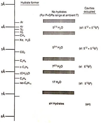
One of the base hypothesis of the model of van der Waals and Platteeuw (1959) which describe the occupancy of cavities by gas molecules is to consider that only one molecule can enter inside, and depending on their side, their affinity varies from one type of cavity to another one. A comparison of guest molecule sizes and cavities sizes is showed on Figure 5 by Sloan and Koh (2007), modified from an original publication of Von Stackelber (1949).
The interest of this figure is to give an indication of the best cavity for each type of gas molecule.
Figure 5 Comparison of guet molecule sizes and cavities occupied as simple hydrates (Sloan and Koh, 2007)
2.4. NUMBER OF HYDRATION
From a given structure, and assuming a full occupancy of cavities, it is possible to give the hydratation number of structure, the number of water molecules per number of gas molecule.
_ _
_
_ _
Number molar water n hyd
Number molar gas
(1)
With 46 water molecules per unit cell, for a total number of 8 cavities, the number of hydration of structure SI is 46/8=5.75. The number of hydration of structure SII is 136/24 = 5.67. For Structure SH, the maximum number of hydration is 34/6 = 5.67
But, full occupancy of cavities is never the case, because sometimes big gas molecules can occupy only the largest cavities, and also because the cavities are not fully occupied. The Table 2 presents a set of experimental data.
Table 2 Hydration number for simple hydrates of natural Gas components from Handa (1986a,b) Component n reference Methane 6.0 Handa(1986a,b) 5.99 Circone et al.(2006) 5.77 Glew (1962) 7.0 Roberts et al. (1941)
7.18 Deaton and Frost (1946)
6.0 Galloway et al. (1970)
7.4 De Roo et al. (1983)
6.3 De Roo et al. (1983)
Ethane 7.67 Handa(1986a,b)
7.0 Roberts et al. (1941)
8.25 Deaton and Frost (1946)
8.24 Galloway et al. (1970)
Propane 17.0 Handa(1986a,b)
5.7 Miller and Strong (1946)
17.95 Deaton and Frost (1946)
18.0 Knox et al. (1961)
17.0 Cady (1983a)
isobutane 17.0 Handa(1986b)
17.1 Uchida and Hayano (1964)
17.5 Rouher and Barduhn (1969)
2.5. MOLAR VOLUME OF GAS HYDRATES
The molar volume of hydrates can be defined to the mole number of water molecules in the hydrate, or in relation to the mole number of gas molecules.
If it is defined to the mole number of water molecules, the molar volume is constant and depends only on the structure. For example, the molar volume of SI structure, composed of 46 water molecules with a lattice parameter of 12.03 Å is (Assane, 2008):
3 (12.03.10 ) 46 H water a m N V (2)
Where N is the Avogadro number (a N = 6.02x10a 23 molecules / molar)
In the other definition, the molar volume of the hydrate follow mole of gas is calculated as:
. _ H gas H water
m m
V V n hyd (3)
where n_hyd is the hydration number.
In the Table 3 we present different properties of hydrates CO2 and CH4 at temperature of
274oK.
Table 3 Molar volume and density of hydrates CO2 and CH4 (Assane, 2008)
consists CO2 CH4
Number of molecules in the unit cell 46
Structure and Volume unit cell (Å 3) SI,1741
Density ideal (kg/m3) 980 912.5
Real number hydratation real at 274 K and Peq 6.24 6.05
Real density at 274 K and Peq (kg/m3) 1099.5 906.4
Molar volume per molecule water (m3/mol) 2.28x10⁻⁵
Molar volume per molecule gas (m3/mol) 1.31x10⁻⁴
Real molar volume at 273 K and Peq (kg/m3) 1.42x10⁻⁴ 1.38x10⁻⁴
3. GAS
PHASE
To calculate the equilibrium parameters, the fugacity coefficient components of the gas
phase have to be determined. It can be calculated using thermodynamic relations at the pressure P (Danesh, 1998).
0 ln ln f P Z 1 dP P P
(4)Where, Z is the compressibility factor. In this study we used the equation of state
/ ( ) c / ( )
P RT v b a v v b (5)
Where v is the molar volume and a and b are constants that depend on the nature and c
temperature of the gas. The a ,b parameter can be calculated using a modified equation of the c
Van Der Waals equation:
2 2 0,42747 C c C R T a P (6) 0,08664 C C RT b P (7) And
0.5
2 1 m 1 Tr (8) With r c T T T (9)Where TC and PC are respectively the critical temperature and critical pressure of the gas. m
was crrolated with the acentric factor by equating fugacities of saturated liquid and vapour at Tr=0.7. (Ali danesh, 1998).
2
0.048 1.574 0.176
m (10)
To solve the equation of state Eq.(5), the constants used are listed in Table 4 Table 4 Constants for calculating the fugacity of gas.
Gas PC (bar) TC (K) ω (-) CO2 72.8 304.2 0.2667 N2 33.5 126.2 0.0372 CH4 45.4 190.6 0.0104 C2H6 48 305.41 0.0979 C3H8 42.4 369.77 0.1522 C4H10 37.84 425.1 0.1995
After rearrangement of the SRK equation of state, we have the compressibility factor is the solution of a cubic function:
Note: in the case of gas mixtures use peudocritical values. Ankur produced a method for calculate, see example below for calculating pseudocritical temperature and pseudocritical pressure
Table 5 example for calculating pseudocritical temperature and pseudocritical pressure
Calculation of Pseudocritical Temperature & Pressure for a Gas Mixture:
Component description Mole Fraction , yi Component Critical Temp., Tc, °K Pseudo-critical Temp, Tpc, °K Component Critical Pressure, Pci, atmA Pseudo-critical Pressure, Ppc, atm Compon ent Molecula r weight, Mi Mixture Molecular weight, yi*Mi CH4 0,932 190,6 177,64 45,35 42,27 16,04 14,95 C2H6 0,058 305,33 17,71 48,07 2,79 30,07 1,74 C3H8 0,01 369,83 3,70 41,92 0,42 44,1 0,44 0,00 0,00 0,00 0,00 0,00 0,00 0,00 0,00 0,00 0,00 0,00 0,00 0,00 0,00 0,00 0,00 0,00 0,00 1,000 Tpc = 199,05 Ppc = 45,47 Mmix = 17,13
3 2 2 0
Z Z A B B Z A B (11) Constants A and B is determined respectively by:
2 2c a P A R T (12) b P B RT (13)
The equation (11) can be solved iteratively or algebraically. We can define new constants Eq((15)(16)) (Bonnefoy 2005). From equation general cube (14)
3 2 0 Z pZ qZ r (14) 3 3 p m q (15) 3 2 9 27 p pq n r (16) 2 3 4 27 n m (17) If > 0, then Z is given 1 1 3 3 3 2 2 p n n Z (18)
If < 0, the compressibility factor is obtained from a different expression :
2 cos
3 3 3
p m
Z
(19)
where is the angle calculated from cos
27324
n n
n m
(20)
In the case of = 0, the fugacity is given
ln A ln 1 B ln Z B Z 1
B Z
Thus, if the acentric factor is known, the critical properties of the gas temperature and pressure, it is possible to determine the compressibility factor, Z, after the fugacity and, finally, the transience of gas. The solubility of gas in liquid phase will be present in section 4.
4. THE
SOLUBILITIES
OF
THE
GASES
IN
THE
LIQUID
PHASE
The gaseous components are dissolved in a liquid phase prior to be crystallized in the hydrate phase. The liquid phase can be both an hydrophilic phase, for example TBAB solution in water, or an hydrocarbon phase, such as cyclopentane when cyclopentane is used as a thermodynamic promoter.
Upon being dissolved in an aqueous phase (L ), COw 2 molecules do partially undergo
acid-base type of chemical reactions: the neutral H CO molecules, the ionic species 2 3 HCO3 and
2 3
CO are formed in the aqueous liquid phase. However, chemical species other than
2
CO (aq) do only exist in negligible amounts (26). In the P–T region of interest, the influence of the speciesHCO (aq)3 , CO (aq)23 ,H CO on the solubility of CO2 3 2 is negligible (Scharlin,
1996). Thus, the condition of thermodynamic equilibrium for CO2 reduces to the phase
equilibrium condition given in eq(22). Expressed in terms of the fugacity Lw
j
f , the phase equilibrium condition reads:
w w hc hc L ( , , L ) L ( , , L ) G( , , ) j j j f T p x f T p x f T p y (22) In eq. (22), Lw( , , Lw) j f T p x , Lhc( , , Lhc) j f T p x and G( , , ) j
f T p y denote the fugacities in the liquid aqueous phase (L ), in liquid organic phase (w L ) and in the gas phase (G ) hc
respectively, for the component j.
The fugacity of components in the liquid phases L and w L are given by an extended HC
form of Henry’s law.
w w w w w L L L , L L H, j, w ( , , ) ( , ) j j j f T p x x k T p (23) hc hc hc hc hc L L L , L L H, j, CP ( , , ) ( , ) j j j f T p x x k T p (24) In eq. (23) and eq.(24), the component solubility is considered to be sufficiently low to define the activity coefficient , L or Lw hc equal to unity in the two liquid phases and to assume
that interactions between both liquids are negligible. The liquid phase is considered incompressible. The pressure dependence of Henry’s constant can be expressed by means of a Poynting correction in the form of the eq. (25).
m, , H, ,j s( , ) H, ,j s( , oj )exp j V p k T p k T p RT (25) In eq.(25), , H, ,j s( , oj ) k T p and m, j
V denote the Henry’s constant of gas j in solvent at
saturation condition prevailing at liquid-vapor phase equilibrium of the pure solvents and partial molar volume of gas j in solvent s, respectively.
m, j
V =32 cm3.mol-1 is the partial molar volume of the gas in water from Holder et al (1980).
,
H j
K , is also calculated here from the correlation of Holder et al (1980):
, H j B K exp A T (26)
Where A and B are constants, given in Table 6
Table 6 Coefficients for the calculation of the Henry constant, from Holder(1980)
Gas A B CO2 14.283146 -2050.3269 N2 17.934347 -1933.381 CH4 15.826277 -1559.0631 C2H6 18.400368 -2410.4807 C3H8 20.958631 -3109.3918 n-C4H10 22.150557 -2739.7313
5. EXPERIMENTAL
EQUILIBRIUM
POINTS
5.1. MATERIALS OF EXPERIMENT
In this work, we used bottles of the individual gases CO2, CH4, C2H6, C3H8, C4H10,
provided by Air liquide. The water is de-ionised from the MILLI-Q 185 PLUS system
(IONEX). In the liquid phase contains LiNO3 as a tracer (10ppm weight fraction).
Table 7 Compositions of the gas use for experiments
Impurity CO2 N2 CH4 C2H6 C3H8 C4H10 H2O < 7ppm < 3 ppm < 5 ppm < 5 ppm < 5 ppm < 5 ppm C2H6 - - < 200 ppm - - - CnHm < 5 ppm < 2 ppm < 50 ppm < 25 ppm < 200 ppm - CO < 2 ppm - - - - - CO2 - - < 10 ppm < 5 ppm < 5 ppm < 20 ppm O2 < 10 ppm < 0.5 ppm < 10 ppm < 10 ppm < 10 ppm < 10 ppm H2 < 1 ppm - < 20 ppm < 40 ppm < 40 ppm - N2 < 25 ppm - < 200 ppm < 40 ppm < 40 ppm < 40 ppm 5.2. PREPARATION OF GAS MIXTURES
Mixtures studied in this study are hydrocarbon and carbon dioxide (CH4 ,C2H6 C3H8, n-
Table 8 Theoretical request for composition of gas mixtures
Gas Gas 1 Gas 2 Gas 3 Gas 4 Gas 5 Gas 6
CO2 - 1 0,2 0,06 - -
CH4 1 - 0,8 0,91 0,95 0,86
C2H6 - - - 0,03 0,03 0,05
C3H8 - - - - 0,02 0,06
n-C4H10 - - - 0,03
Two methods are used to prepare the gas mixture, one consist in preparing directly the mixture in the reactor, the other in preparing the gas mixture outside, in a preparation room, and to feed the reactor directly with a bottle of the gas mixture.
- Case 1: Bottles of each gas are directly connected to the reactor (Experiments No. 4, 5 in Figure 6). The mixture is made by a sequential injection of the gases into the reactor which has been previously vacuumed. The quantities of gases is controlled from the pressure monitoring and the knowledge of the exact composition is validated by gas chromatography. The mass balance is made from a method given in section. This method has been used for binary mixtures.
- Case 2: For all other gas mixtures (more than two gas), an external gas bottle has been prepared in a preparation room, also by successive injections of each gas, from less volatile to more volatile, by controlling the pressure. At each step, the composition is determined from a weighing with a balance of 0.1 g precision. The final composition is cross validated by gas chromatography.
Due to the methods, it is difficult to get exactly the compositions specified in Table 8. The final composition is given in Table 11.
5.3. EXPERIMENTAL SET-UP
The experimental apparatus (Figure 6) is designed to measure the thermodynamic equilibrium points in presence of gas mixture and to determine the composition of all phases (gas, liquid and hydrate). The reactor consists of a 2.36 liter autoclave reactor in which the pressure can reach up to 100 bars. The reactor is equipped with two vertical stirrers with four
blades, one in the liquid, one in the gas. The stirring rate can vary between 0 and 600 rpm. The temperature is controlled by a double jacket in which is circulated a fluid at constant temperature from a cryostat HUBERT CC-250. A Pyrex cell is laid inside the reactor and filled with water containing Lithium as an anion tracer. The liquid is injected in the reactor under pressure by using a HPLC pump (JASCO). Temperature is monitored by two Pt100 probes, one in the gas phase, the other in the liquid phase. The pressure is measured with an accuracy of 0.01 MPa in the range 0-10 MPa. A ROLSI sampler is mounted on the reactor. It allows to sampling online the gas and to sending the sample into a gas chromatograph (GC Varian model 38002) equipped with a TCD detector and two columns PoraBOND Q and CP-Molsieve. The peak integration is possible with software provided by Varian Galaxie. Another sampling system can exit the liquid phase through a mechanical valve and a capillary tube. The liquid is analyzed off-line by ion chromatography. The data acquisition is controlled on the personal computer.
Figure 6 Experimental device
5.4. EXPERIMENTAL PROTOCOL
Initially, the reactor is cleaned with water and evacuated by a vacuum pump for 40 minutes. Then, depending on the case (see section 5.2), the pure gases are directly injected
into the reactor from pure gas cylinders (CO2 and CH4), or from a bottle prepared previously
at the good composition. In each case, the first injection of gas is repeated three times after a purge under vacuuming, to ensure that air is totally evacuated.
The temperature is initially set with the thermostat at the value of 1°C. The control of temperature takes into account a difference between the temperature of the glycol solution circulating in the jacket, and the effective temperature in the reactor which is around the value of 1.5°C higher, but depends on the room temperature.
The experiments are realized following 3 steps
Step 1: Injection of the pure gas, or gas mixture, following the procedure given in 5.2 (case 1 or case 2). The stirrer is on. The composition of the gas is controlled via gas chromatography.
Step 2: Injection of water: The stirrer is stopped. The water solution containing 10 ppm molar fraction of LiNO3 (tracer) is prepared and injected via the HPLC pump with the amount of 800 g measured by a mass balance. Pressure and temperature increase due to the gas contraction volume. Then, the pressure decreases because a fraction of the gas dissolves in the liquid phase. The temperature also decreases because to reach the operative temperature controlled by the cooling jacket. Agitation is restarted, and the evolution of the temperature and pressure in the reactor is monitored. After a delay corresponding to the induction time, ranging from minutes to hours (nucleation is a stochastic phenomenon), the crystallization starts, gas is consumed and the pressure is dropped down to the equilibrium. It is accompanied by a temperature increase due to the exothermic character of the crystallization. During formation of the solid phase, the pressure decreases because it consumes gas. The crystallization is occurring during hours and days, during which the gas phase is sampled on-line. The liquid phase is also sampled and analyzed later (off-lines).
Step 3: Dissociation of hydrates: when the system is at equilibrium (temperature and pressure are stable), the reactor is heated by steps of 1°K until a full dissociation of hydrates (Figure 8). At each stage of dissociation, a gas sample is taken with the sampler ROLSI and it is sent to the gas chromatograph (on-line) to determine the gas compositions in gas phase. The liquid is also sampled to determine the concentration of Lithium in the water, after off line analysis in an ion chromatography. During each step, the pressure in the reactor increases due to the dissociation of hydrates and reaches a constant value which is considered as the thermodynamic equilibrium. This step is repeated until total dissociation. After a
complete dissociation, the pressure in the reactor continues to increase but only in respect to the dilatation of gases and decrease of the solubility of gases.
Figure 7 Evolution of pressure and temperature during the Crystallization
Figure 8 Evolution of pressure and temperature during the dissociation
5.5. CALIBRATION OF THE GC DETECTOR
In these studies the gas Chromatograph used is the Varian 3800 GC model, the gas chromatograph allows us to know the composition of a gas mixture. In fact, the area of a
given peak of component A in the chromatogram is proportional to the amount of material (nA) in the sample.
A A A A T A
S k n k n x (27)
T
n represents the number of moles of all the species, and xAis the molar fraction of
component A. kA is a constant of proportionality which can be determined experimentally if
the amount of A is known. But, in our experiment, the amount of component can not be determined after sampling due to the sampling method. In fact, the Rolsi instrument is a valve that is opened during a period of time. During this period, the amount of material is proportional to the flow rate, and the flow rate is directly proportional to the pressure. The pressure is not a process control parameter, but is dependent from equilibrium considerations, for example the temperature.
So, we need to use a relative calibration method, by taking a gas as a reference, here the methane because it is the higher composition component, in general:
A A A A T A S k n k n x (28) 4 4 4 4 4 CH CH CH CH T CH S k n k n x (29) 4 4 4 , A A A CH CH CH S k x S x (30)
The calibration curves are presented in the form of the straight lines with different slopes (KA CH, 4 1 kA CH, 4 ) and given in Figure 9 to Erreur ! Source du renvoi introuvable..
Once the KA CH, 4constants have been determined, for a given gas mixture, the gas composition
is given by the following equations:
4 4 4 4 , 1 1 CH A A CH A CH CH x S K S
(31) 4 4 4 4 , A A CH CH A CH CH S x x K S (32)5.5.1 Calibration of CO2
Table 9 Results of the calibration of gas chromatography (CO2-CH4)
P(CO2)
bars
P(CH4)
bars
X(CO2)/X(CH4)
from mass balance, case 1, §5.2
S(CO2)/S(CH4)
from gas chromatography
X(CO2)/X(CH4) from
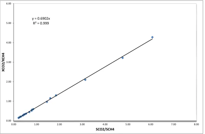
GC and Eqs.(31) and (32) Erreur (%) 19.9 5.6 4.28 6.07 4.44 2.89 15.6 5.6 3.22 4.77 3.48 5.87 10.6 5.6 2.10 3.13 2.29 5.84 10.5 7.9 1.30 1.85 1.35 2.21 6.2 5.3 1.15 1.60 1.17 0.70 5.1 5.6 0.97 1.45 1.06 4.60 6.2 10.2 0.59 0.85 0.62 1.93 10.5 17.9 0.56 0.80 0.58 1.30 10.8 19.9 0.52 0.79 0.57 3.65 10.8 23 0.44 0.68 0.50 3.65 10.8 28 0.36 0.54 0.40 2.62 10.5 29.3 0.33 0.49 0.36 1.61 6.7 20.1 0.32 0.46 0.34 1.52 6.2 18.9 0.31 0.44 0.32 0.65 10.5 35.1 0.27 0.41 0.30 2.07 10.8 36.9 0.27 0.40 0.29 1.73 6.7 29.6 0.21 0.32 0.23 1.68 6.3 29.5 0.20 0.28 0.20 0.21 6.2 29.2 0.20 0.28 0.21 0.74 6.7 40.1 0.15 0.22 0.16 0.53 6.2 39.8 1.45 0.22 0.20 1.45
y = 0.6902x R² = 0.999 0.00 1.00 2.00 3.00 4.00 5.00 6.00 0.00 1.00 2.00 3.00 4.00 5.00 6.00 7.00 8.00 XC O2 /X CH4 SCO2/SCH4
Figure 9 Calibration curve of the gas chromatograph for CO2-CH4
5.5.2 Calibration of C2H6 y = 0,678x - 0,000 R² = 0,995 0 0,05 0,1 0,15 0,2 0,25 0 0,05 0,1 0,15 0,2 0,25 0,3 0,35 X( C2 H6 )/ X( CH 4) S(C2H6)/S(CH4) C2/C1
y = 0,385x + 0,001 R² = 0,990 0 0,01 0,02 0,03 0,04 0,05 0,06 0,07 0,08 0,09 0 0,05 0,1 0,15 0,2 0,25 XC 3H 6/ XC H4 SC3H6/SCH4 C3/C1
Figure 11Calibration curve of the gas chromatograph for C3H8-CH4
5.5.4 Calibration of C4H10 y = 0,270x + 0,000 R² = 0,972 0 0,005 0,01 0,015 0,02 0,025 0,03 0,035 0,04 0 0,02 0,04 0,06 0,08 0,1 0,12 0,14 0,16 XC 4H 10/ XC H4 SC4H10/SCH4 C4/C1
5.6. EXPERIMENTAL RESULTS
In this section, we present our method to calculate the mass balance, and evaluate the hydrate composition as a function of the gas composition at a given temperature and pressure. We give also the experimental results under the form of figures and tables.
5.6.1 Calculation of the composition in the different coexisting phases
To calculate the mole number of each gas in the different coexisting phases, a mass balance is
used. Notes 0
j
n is the amount of initial and molecule total gas j in the reactor:
0 G L H
j j j j
n n n n (33)
Where exhibitors G, L and H correspond to gas phase, liquid and hydrate. And:
- G j
n the number of moles of gas j in the gaseous phase, - L
j
n the number of moles of gas j in the liquid phase j,
- H
j
n the number of moles of gas j in the hydrate phase.
The initial quantity of gases in the reactor is finally distributed within the three phases. Before and during the crystallization, or at equilibrium, the composition of gas in the gas phase is determined from a gas chromatography analysis given in Eqs.(31) and (32). The total mole number in the gas phase is calculated from the classical state equation:
0 0
PV ZnRT (34)
Where, Z is the compressibility factor, n is the total mole number of gas molecules. P is the pressure. V0 is the total volume of the reactor (V0 = Vreactor = 2.36 L). T0 is the temperature
(°K) and R is universal gas constant.
• In the gas phase
The number of moles in the gas phase is determined by the classical equation of gas: G
G
PV Zn RT (35)
- P is the pressure in the reactor, - T is the temperature in the reactor,
- VG is the volume of the gas, approximated by VG V V0 w,
- Z is the compressibility factor,
- VwThe volume of water,
- nGis the total number of moles in the gas.
where the compressibility factor (Z) is determined from the critical properties and acentric factor (ω) as explained in section 3. From P, V, T, and the composition of the mixtures gas (by
chromatography), G
j
n is calculated for each gas j.
Note: The volume occupied by the gas is equal to the reactor volume minus the volume of the liquid (≈ water) and hydrate (determined from the Li concentration measurement that gives the amount of liquid water consumed).
• In the liquid phase
At equilibrium, the quantity of gas in the liquid is calculated from two steps, calculation of the volume of remaining water, and calculation of the dissolved components from a gas/liquid model assumption.
Calculation of the volume of water
As mentioned before, the liquid phase (water) contains a tracer LiNO3. Initially the
concentration of lithium [Li+]0 and the initial volume of liquid
0L
V are known (Lithium is about 10 ppm, and water is about 800ml). During crystallization and dissociation steps, the concentration of lithium is measured by ionic chromatography after sampling. So, we can calculate the volume of remaining liquid water by:
L 0 e 0 q V Li V [Li ] L eq (36) 0 0L. L eq eq V Li V Li (37) Where,Lieq
, V are concentration of lithium at equilibrium and volume of water injection 0L