Impact of ocean waves on deep waters mixing and large-scale circulation

HAL Id: tel-01713054

https://pastel.archives-ouvertes.fr/tel-01713054

HAL is a multi-disciplinary open access archive for the deposit and dissemination of sci-entific research documents, whether they are pub-lished or not. The documents may come from teaching and research institutions in France or abroad, or from public or private research centers.

L’archive ouverte pluridisciplinaire HAL, est destinée au dépôt et à la diffusion de documents scientifiques de niveau recherche, publiés ou non, émanant des établissements d’enseignement et de recherche français ou étrangers, des laboratoires publics ou privés.

Impact of ocean waves on deep waters mixing and

large-scale circulation

Oceane Tess Richet

To cite this version:

Oceane Tess Richet. Impact of ocean waves on deep waters mixing and large-scale circulation. Other [cond-mat.other]. Université Paris-Saclay, 2017. English. �NNT : 2017SACLX104�. �tel-01713054�

THESE DE DOCTORAT

DE L’UNIVERSITE PARIS-SACLAY

préparée à

L’ÉCOLE POLYTECHNIQUE

Laboratoire d’hydrodynamique de l’Ecole polytechnique

ÉCOLE DOCTORALE N°579

Sciences Mécaniques et Energétiques, Matériaux et Géosciences (SMEMaG)

Spécialité de doctorat : Mécanique des fluides

par

Océane Richet

Impact of ocean waves on deep waters mixing and

large-scale circulation.

Thèse présentée et soutenue à Paris, le 06 Décembre 2017. Après avis des rapporteurs :

Chantal Staquet (LEGI)

Sonya Legg (GFDL - Princeton University)

Composition du jury :

Pascale Bouruet-Aubertot (LOCEAN) Présidente du jury Chantal Staquet (LEGI) Rapportrice Sonya Legg (GFDL) Rapportrice Jean-Marc Chomaz (LADHYX) Directeur de thèse Caroline Muller (LMD-ENS) Co-directrice de thèse Sabine Ortiz (IMSIA) Examinatrice

Impact of ocean waves on deep waters

mixing and large-scale circulation

prepared by

Océane Richet

under the supervision of

Caroline Muller and Jean-Marc Chomaz

Je ne peux que commencer par vous remercier Caroline et Jean-Marc. Sans vous rien de tout cela n’aurait eu lieu. Merci de m’avoir donnée ma chance. Et puis commencer une thèse par un entretien dans un café ça ne présageait qu’une bonne ambiance (de travail) ! J’ai adoré travailler avec vous deux. A tous les 3 on forme une bonne équipe ! C’était très enrichissant d’avoir vos deux points de vue. Vous m’avez également donnée la possibilité de vraiment découvrir le monde de la recherche au travers de toutes les conférences, des échanges avec d’autres labo, des écoles d’été et tout simplement au travers vos propres expériences. J’espère qu’on aura encore l’occasion de travailler ensemble, ou juste d’aller boire un verre de temps en temps !

Bêêêêêêêêêh !!!!! Bêêêêêh !!!!! Baaaaalle !!!! Bêêêêêh !!!!! Balle aléatoiiiiiiire !!!! Voilà ce qui se cache derrière la porte du bureau invisible ! Une bonne thèse ne va jamais sans de géniaux cobureaux ! Merci Gaétan de m’avoir fait visité le Ladhyx pour me convaincre de venir. Finalement, tout s’est joué lors du lâché de ballon devant le labo ! Merci aussi d’avoir fait irruption dans le bureau pour la fin de ta thèse, tu as bien élevé le niveau des conversations au son de tes bêêêêêêh ! Merci Julien et Tristan d’avoir été mes premiers cobureaux pour entamer cette longue épreuve au milieu de tous ces X et au bout du monde. Merci Guillaume et Elizabeth pour vos sacrées Munstiflettes et Tartiflettes ! Je retiendrai les lardons cuits au beurre. Merci Léopold pour avoir toujours envie de jouer à la balle et de veiller à ce qu’on ait notre quota de sport par jour ! Merci Vincent pour avoir remplacé Guillaume même si on ne sait toujours pas si tu es un espion du préfa ou si tu as fini par prêter allégeance aux numériciens. Merci Tristan pour avoir été souvent partant pour me suivre dans mes weekends rando improvisés et finalement revenir plus fatigués qu’avant le weekend. Sans toi je me serai sentie un peu seule comme lève tard et comme profiteuse de grands weekends. Il te reste une mission : prendre soin de Charlotte en espérant qu’un jour elle refleurisse! Je rajouterai merci Eunok pour tes passages furtifs dans le bureau. Merci pour ces weekends au soleil à regarder les poulpes. Et oui, un jour on aura notre château plein de chats sur la corniche à Marseille !

Bien sûr, je n’oublie pas toutes les autres personnes du ladhyx que je remercie. Vous avez tous participé à cette super ambiance au labo. Notamment le préfa avec toutes vos inventions un peu folles mais toujours super utiles. D’ailleurs j’espère bien un jour goûter à une de vos pizzas ! merci aux personnes de "l’autre bâtiment" d’avoir répondu à mes quelques invitations pour réunir tous les thésards du labo autour d’un bon repas au resto ! En tout cas, je ne pouvais pas rêvé plus enrichissant que d’être dans un labo aussi diversifié.

Mes petits chats, merci de m’avoir fait une place dans votre bureaux ! Vous êtes les meilleurs cobureaux pour finir une thèse !!!! Tout autre ambiance que celle au ladhyx mais tout aussi sympathique ! A vous, monsieur Perrot et monsieur Laxenaire. Merci aussi à Claire qui a tenté de me motiver à aller faire du sport. Bon on n’a pas été super efficaces mais la volonté était là ! Raphaela, that was so nice to meet you at the MIT. I loved the time I spend with you to listen classic music, to discover Boston and our long chats under the sun! I remember our cycling

vi

trip, the snake on the road and the well-diserved hot chocolate at the end! You illuminated my time in Boston. Qi, you was the best roomate ever but also my favorite big sister! You are petite but so funny!!!! I enjoyed our girl talks and to discover China through you! You are a great chef! Thank you to teach me how to cook your famous dumpling!

Et puis, il y a vous tous, mes petites cacahuètes, ma famille de substitution depuis toutes ces années : Valérie (cacahuète number one), Anne So, Chlochlo, Miloune, Stefan, Anaïs, Mot Mot, Marthouille, Clara, Rafiki ! On en a partagé des choses entre nos diners de retour de vacances et de Noël, les soirées jeux et les aventures dans lesquelles je vous ai souvent entrainés ! Cacahuète, Anne So, Chlochlo, Anaïs et Mimi, heureusement que vous étiez là quand j’étais toute tapata, comment est-ce que j’aurais pu survivre sans vous ?! Cacahuète, j’espère que dans 10 ans et même plus encore on arrivera à se retrouver pour nos goûter blabla à la Jacobine ! Anne So, je compte sur toi pour toujours avoir une bonne bière au frais au cas où je débarquerai. Au pire on ira pécher des crocodiles ! Chlochlo, que dire à part qu’on a vaincu la monté de la mort ensemble, les sapins et les bouquetins s’en souviennent encore ! Anaïs, mini cacahuète à l’emploi du temps de ministre, n’oublies pas que l’on doit toujours partir en vacances ensemble ! En attendant je suis très fière de te prêter mon anniversaire pour ta soutenance ! Ma Miloune d’amour, j’ai tellement de choses à raconter, au moins de quoi écrire une nouvelle thèse ! En même temps ça fait 12 ans que l’on parle de nourriture, ça n’est pas rien ! Mot Mot, à nos conversations jusqu’au petit matin à finir toutes ces bonnes bières alors que tout le monde a déserté depuis un bout de temps ! Clairement le temps n’avance pas pareil entre minuit et 6h du matin ! Tu as toujours été là pour écouter mes histoires. Marthouille, ma petite Marthemotte, promis la prochaine fois je te ferai une rando avec juste des plats et des descentes ! Clara, heureusement que tu étais là pour programmer et organiser nos soirées jeux et diners ! Ça représente plein de souvenirs mais au jour le jour, dans une thèse, ces moments passés avec vous sont des grandes bouffées d’air et de fous rire ! Une thèse ce n’est rien si on n’a pas les amis qui vont avec, le reste du temps !

Doubi, merci de m’avoir supportée tout ce temps et surtout merci de continuer à être là pour moi. Tu es souvent mon sauveur lors de mes petites galères de thèse ! Tout ça compte énormément pour moi et j’espère que j’arrive à te rendre la pareille !

Un grand merci à toute ma famille qui est derrière moi depuis toutes mes années étudiantes. Votre soutien a été indispensable dans ce travail de longue haleine même si je sais que pour la plus part d’entre vous je parle chinois et que ma vie ressemble plus à carnet de voyage ! Je vous dois beaucoup pour en être arrivée jusque là ! Je vous remercie d’être toujours présents même quand je suis au bout du monde (ce qui arrive finalement plus souvent que prévu) !

Tilili ! Tilili ! Tililiiiiiiiiii !!!!!!! TILILILILILILILILILILILILILILILILILI

(\ (\ ( -.-)

Preamble 3

1 Introduction 7

1.1 Ocean water masses: description . . . 8

1.1.1 The oceanographers’ view . . . 8

1.1.2 North Atlantic Deep Water . . . 10

1.1.3 Antarctic Bottom Water . . . 13

1.1.4 A 3D ocean . . . 14

1.2 Meridional overturning circulation: pushed of pulled? . . . 18

1.2.1 The school of pushing: Deep water formation pushes the deep current . . . 18

1.2.2 The school of pulling by deep mixing: Deep mixing removes cold water from the abyss . . . 19

1.2.3 The school of pulling by wind stress: The Southern westerlies pull cold water from the deep ocean . . . 21

1.2.4 Combination of the two schools of pulling . . . 24

1.3 Waves . . . 26

1.3.1 Stratified ocean: the Brunt Väisälä frequency . . . 26

1.3.2 Internal gravity waves . . . 27

1.3.3 Kelvin and topographic Rossby waves . . . 32

2 Internal tide dissipation at topography: triadic resonant instability equator-ward and evanescent waves poleequator-ward of the critical latitude 37 2.1 Introduction . . . 38

2.2 Methods . . . 40

2.2.1 Theoretical background: equations of motion . . . 40

2.2.2 Numerical simulations configuration . . . 41

2.3 Overview of numerical results: latitudinal distribution of tidal dissipation and physical processes involved . . . 43

2.4 Part I - Equatorward of the critical latitude: Triadic Resonant Instabilities (TRI) . 46 2.4.1 Stage I: TRI . . . 46

2.4.2 Stage II: accumulation of inertial waves . . . 49

2.4.3 Stage III: dominant TRI . . . 52

2.4.4 Evolution of dissipation from the equator toward the critical latitude . . . . 54

2.5 Part II - Poleward of the critical latitude: evanescent waves . . . 55

2.5.1 Theory of PSI extension . . . 56

2.5.2 Numerical results . . . 57

2.6 Discussion and conclusions . . . 58

x Contents

3 Impact of a Mean Current on the Internal Tide Energy Dissipation at the

Critical Latitude 61 3.1 Introduction . . . 62 3.2 Methods . . . 65 3.2.1 Numerical model . . . 65 3.2.2 Settings . . . 66 3.2.3 Topography . . . 67

3.2.4 Tidal and mean currents imposed . . . 68

3.3 Results: realistic topography . . . 69

3.3.1 Control case: tidal energy transfer without mean current . . . 69

3.3.2 Impact of a mean current on energy dissipation . . . 73

3.3.3 Kinetic energy spectrum and Doppler effects . . . 75

3.4 Results: sinusoidal topography . . . 79

3.5 Conclusions and discussion . . . 82

4 Influence of upstream perturbations on upstream circulation of a hydraulically controlled sill 87 4.1 Introduction . . . 88

4.2 Methods . . . 89

4.3 Preliminary numerical results: dam break . . . 91

4.3.1 Circulation in the basins . . . 91

4.3.2 Hydraulic control in the channel and transport . . . 92

4.3.3 Waves induced by the dam break . . . 93

4.3.4 Influence of parameters (∆ρ, latitude, sill depth and slope) on Froude number and transport . . . 94

4.4 Dam break simulation with a northern inflow . . . 95

4.4.1 Circulation in the upstream basin . . . 96

4.4.2 Froude number: hydraulically controlled? . . . 98

4.4.3 Transport through the channel . . . 98

4.4.4 Waves induced by the inflow and the dam break . . . 100

4.5 Perturbation of the northern inflow . . . 101

4.6 Discussion and conclusion . . . 102

5 Main results of the thesis and perspectives 105 5.1 Conclusions on the projects . . . 106

5.2 Future work . . . 107

Appendices

A Growth rate calculations 113

B PSI extension calculations 119

C Mean current 123

Bill Watterson, 23 July 1987

In the context of global warming, the ocean is the main receptacle having absorbed more than 90 % of the anthropogenic energy surplus. The effects induced by the warming become detectable and impact the structure of the ocean, its circulation as well as atmospheric [Lambaerts et al. 2013] and oceanic ecosytems [Villar et al. 2015]. A better understanding of the local and global oceanic circulation will permit to improve the predictions from global climate models.

To gain better fundamental understanding of the ocean, it is natural to begin by describing the structure of the ocean and to introduce the concept of water mass. This vision of the ocean is a schematic vision of the ocean used by oceanographers to understand the exchanges between the different basins. A brief description of the two principal water masses relevant for this study is given in chapter 1.

This project encompasses oceanic motions at very different time scales. These include slow time scale of the thermohaline circulation, a quasi static vision of the ocean. Other faster processes, like winds, tides or waves, play an important role in maintaining the overturning circulation. A description of the diverse theories for the global overturning circulation is given in chapter 1, allowing to introduce

4 Contents

the role of waves in maintaining and modulating the oceanic circulation.

At this point, a physical description of the oceanic waves, involved in the studies presented in this thesis, is salutary for the rest of the manuscript. The end of chapter 1 thus details the specific conditions for the development of internal waves and more specifically of internal tides, Kelvin waves and topographic Rossby waves, and their principal characteristics.

This introduction to the global context of the study is followed in chapter 2 by a first study on the mechanisms leading to the dissipation of the internal tides (also called baroclinic tide) in an idealized ocean. Internal tides are internal waves at the tidal frequency generated by the action of the barotropic tide in a stratified fluid. In this study, we focus on the semi-diurnal lunar tide (M2) interacting with a sinusoidal topography in a 2D high resolution numerical model. This study has been submitted for publication in the Journal of Geophysical Research: Oceans.

Once the mechanisms behind the dissipation of internal tides are clarified, we study in chapter 3 the effect of a background mean current like mesoscale eddies or large-scale currents, on the latitudinal distribution of internal tide energy dissipation. Using a 2D numerical model and, a realistic or an idealized rough topography, we impose a weak mean current which does not affect the generation of internal tides. The results of this study have been published in the Journal of Physical Oceanography.

The last chapter is part of an ongoing research project developed at the Geophysical Fluid Dynamics summer school (Woods Hole) in collaboration with Renske Gelderloos, Larry Pratt and Jiayan Yang. The problem of water export from a marginal sea toward open ocean is well known in oceanography. In this study, we propose to investigate how upstream disturbances influence the upstream circulation of a hydraulically controlled sill in a 1.5-layer reduced gravity model. This study is still in preparation and will be published in the near future.

The last chapter summarizes the key results of this thesis, and provides a discussion of ongoing and future work.

1

Introduction

Bill Watterson, 24 July 1987

8 1.1. Ocean water masses: description

1.1

Ocean water masses: description

The ocean is something that most of people know and have experienced someday at the beach. The first contact teaches, right away, that the ocean is a salty fluid with a varying temperature: warmer at the surface and colder at depth. Once the swim is over, it has happened to many of us, wistfully gazing out the ocean, to realize how vast and unknown it is.

To improve our common vision of the ocean, most of the time restricted to the coast, oceanographers do measurements all over the world revealing what is under the surface. Through the measurements of temperature, salinity, oxygen and other tracers, they give a global vision of the time varying structure of the ocean.

1.1.1

The oceanographers’ view

The ocean is a stratified fluid whose density varies with temperature and salinity

of the fluid. The densest fluids (cold and salty) fill the bottom and lightest

fluids (fresh and warm) are at the surface. A variation of temperature can be induced, for example, by interaction with atmosphere or geothermal fluxes. On the other hand, salinity varies with precipitation/evaporation, fresh water from rivers or formation/melting of sea ice. The different forcings correspond globally to the thermohaline forcing.

These processes are not homogeneous in space and time, which induces variations of temperature and salinity, and thus density in the ocean. In order to understand the structure of the ocean, oceanographers develop the concept of water masses. A water mass is an identifiable body of water with a common formation history whose physical properties (temperature and salinity, among others) are distinct from surrounding water. Each water mass has a name reflecting its origin and its depth location. Commonly in oceanography, we use their acronyms and the first summary and review is given by [Emery and Meincke 1986]. We first restrict the discussion to the Atlantic basin, before moving on to the circulation between four connected basins.

Figure 1.1 shows the same meridional section of the Atlantic for potential

temperature 1_{, salinity and neutral density}2_{. In these figures, we can easily identify}

1_{Potential temperature: temperature of a water parcel that it would acquire if adiabatically}

brought to a standard reference pressure.

2_{Neutral density is a variable commonly used in oceanography to identify water mass. In}

fact, a neutral density surface is the surface along which a given water mass will move, remaining neutrally buoyant. The neutral density is a function of temperature, salinity pressure and time. It

NADW

Surface water

AABW

318MSAVE5 318MHYDROS4 32OC202-1

237314 369 119 Depth (m) 0 100 200 300 400 500 600 700 800 900 1000

CTD salinity for A16 25° W

Depth (m ) 278 275 270 265 260 255 250 245 240 315 320 325 330 335 340 345 350 355 360 365 115 110 105 100 95 90 85 80 75 70 65 60 55 50 45 40 35 30 25 20 15 10 5 2 Station No. 34.94 34.90 35.20 35.30 35.70 36.00 35.50 35.30 35.10 35.04 35.00 34.98 34.96 34.95 34.94 34.92 34.90 34.88 34.72 34.74 34.80 34.86 34.90 34.91 34.90 34.72 34.70 34.88 34.92 34.70 34.40 34.30 34.20 34.80 34.80 34.50 33.90 34.10 34.50 34.60 34.65 34.20 34.30 < 34.40 34.45 34.50 34.60 35.60 35.65 35.70 37.30 37.00 36.20 35.80 35.70 35.60 35.55 35.50 36.00

Figure 1.1: (top) Potential temperature (◦C), (middle) salinity (PSU) and (bottom) neutral density (kg m−3_{) for the Atlantic basin from 54}◦_{S to 63}◦_{N (see medallion). Areas} of surface water, North Atlantic Deep Water (NADW) and Antarctic Bottom Water are roughly defined. From www.woceatlas.ucsd.edu

10 1.1. Ocean water masses: description

areas with similar ranges of temperature and salinity defining their density; they compose the water masses present in the Atlantic Ocean. At first glance, we can identify a warm, salty and light surface water and two cold and salty tongues coming from the north and south edges, corresponding to the formation of dense water in the northern Atlantic and bottom water in the Southern Ocean (southern Atlantic).

All the water masses in the ocean will not be described in the present document, only the two important water masses for our studies: the North Atlantic Deep Water (NADW) and the AntArctic Bottom Water (AABW). These two water masses form the two densest waters in the ocean and play a major role in the overturning thermohaline circulation and in the climate. Indeed, before sinking, they are in direct interaction with the atmosphere permitting, among others, the absorption and sequestration in deep ocean of anthropogenic carbon. The rate of deep water formation can vary strongly with atmospheric condition. Global warming could inhibit deep water formation inducing a slow-down of 20-50% [Rahmstorf et al. 1999] or even a break-down of the thermohaline circulation [Broecker 1987].

1.1.2

North Atlantic Deep Water

North Atlantic Deep Water has a temperature of 2-4◦C, a salinity superior to 34.9

PSU and a neutral density superior to 26.76 kg m−3 (see Fig. 1.1). North Atlantic

Deep Water is well described by Hansen and Østerhus [2000].

North Atlantic Deep Water is mainly formed in the Nordic Seas (Greenland and Norwegian seas) from Atlantic water during strong winters (see Fig. 1.2). The warm and light Atlantic surface water loses heat by exchange with the cold atmosphere. The water becomes colder at the surface and so sufficiently dense to induce a convective movement: the cold surface water sinks and lighter deep water comes up to the surface where it will be cooled (see Fig. 1.3). At the end of the winter, the newly formed dense water fills the bottom of the Nordic Seas. Additionally, water from the Arctic basin enters in the Nordic Seas from the Fram Strait and mixes with the cooled surface Atlantic water acquiring its final characteristics before overflowing equatorward through the Greenland-Iceland-Scotland ridge in the Atlantic basin as a deep water (see Fig. 1.2 - dashed curves on the eastern flank of Greenland).

Figure 1.2: Schematic circulation of surface currents (solid curves) and deep currents (dashed curves) in the North Atlantic and in the Nordic Seas. Colors of curves indicate

approximate temperatures. Figure adapted from [Curry and Mauritzen 2005]._{11.2. THE OBSERVED THERMOHALINE CIRCULATION 237}

FIGURE 11.12. Schematic diagram of the three phases of open-ocean deep convection: (a) preconditioning,

(b) deep convection and mixing, and (c) sinking and spreading. Buoyancy flux through the sea surface is represented by curly arrows, and the underlying stratification/outcrops are shown by continuous lines. The volume of fluid mixed by convection is shaded. From Marshall and Schott (1999).

FIGURE 11.13. Zonal average (0◦_{−→ 60}◦_{W) temperature (top) and salinity (bottom) distributions across the}

Atlantic Ocean. Antarctic Intermediate Water (AAIW), Antarctic Bottom Water (AABW), and North Atlantic Deep Water (NADW) are marked. Compare this zonal-average section with the hydrographic section along 25◦_{W shown}

in Fig. 9.9.

Figure 1.3: Sketch of the three phases of ocean deep convection: (a) preconditioning, (b) deep convection and mixing, and (c) sinking and spreading. Buoyancy flux through the sea surface is represented by curly arrows, and the underlying stratification/outcrops are shown by continuous lines. The volume of fluid mixed by convection is shaded. From [Marshall and Schott 1999].

The export of dense water from the Nordic Seas into the Atlantic basin is controlled by the presence of sills (see Fig. 1.2): the Denmark Strait between

Greenland and Iceland (sill depth 620 m and volume exported 3 Sv, 1 Sv = 106

m3_s−1_{), the ridge between Iceland and Faroe Islands (840 m, 1 Sv) and Scotland}

and the Faroe Bank Channel between Faroe Islands (420 m, 2 Sv). These sills are hydraulically controlled [Whitehead et al. 1974; Nikolopoulos et al. 2003; Girton et al. 2006] which means that the flow upstream of the sill is laminar (river regime)

12 1.1. Ocean water masses: description

492 Thermohaline circulation

basin to the others must go over sills which exist as the lowest passages in these otherwise tall topographic barriers.

When water moves over a sill, it behaves very much like a deep waterfall. In many cases, a deep waterfall involves a volume flux on the order of 1–10 Sv (106₋₁₀7_m3_{/s), and an}

elevation change on the order of several hundreds of meters. Many people have visited the Niagara Falls, one of the largest land-based waterfalls in the world, which has a maximal volume flux of 3,000 m3_{/s and elevation drop of 56 m. In comparison, deep waterfalls are}

much more powerful than any land-based waterfall on Earth, with a volume flux of more than 1,000 times and elevation drop of more than 10 times that of the Niagara Falls.

The meaning of rotating hydraulics

An essential feature common to the overflow associated with deepwater formation is that the overflow goes through the transition from subcritical to critical, and then to supercritical. Whether a flow is subcritical or not is defined in terms of the Froude number. Using the waterfall as an example, the concept of hydraulics for a non-rotating fluid can be explained as follows. For water flowing in an open channel, signals propagate with the velocity of the surface wave, i.e., c=!gh, where h is the depth of water. The Froude number is defined as F = U/c, where U is the horizontal velocity of the fluid. For most cases of flow through a channel, F < 1, so the fluid motion is subcritical, i.e., fluid travels at a speed slower than the speed of signals.

If the mean slope of the channel is gradually increased, fluid speed increases. At a critical value of slope, water travels so fast that its speed exactly matches the speed of surface waves. Generally, the bottom of the channel is not flat, and there is a place in the channel where the depth is the shallowest. This is called a sill, and depth both upstream and downstream from the sill is greater, as shown in Figure 5.8.

Assume that water motion upstream from the sill is subcritical and the depth of the sill is gradually reduced. The Froude number at the sill gradually increases, while flow in the

Signal speed

Flow speed

Subcritical flow Critical flow Supercritical flow

h

Fig. 5.8 Sketch of overflow from a marginal sea to the open ocean, involving rotating hydraulics.

Figure 1.4: Sketch of an overflow from a marginal sea (Nordic Seas) to the open ocean (Northern Atlantic) [Huang 2010].

and downstream of the sill the flow is highly turbulent (torrential regime) 3 _(see

Fig. 1.4). The regime change is induced by a change in the relative importance of the kinetic energy compared to the potential energy of the fluid and quantified by

the Froude number F r = U/√g0_{h, where U is the fluid velocity, g}0 _{= g∆ρ/ρ}

0 the

reduced gravity, ρ0 is the reference density, ∆ρ the density difference between the

two layers and h the fluid thickness, which is the ratio between the kinetic energy and the potential energy. When the Froude number is greater than 1, for supercritical flow, which corresponds to large U , small h, and kinetic energy dominated regime (downstream of sill, torrential regime). When it becomes less than 1, for small U , large h, and hence potential energy dominated regime (upstream of sill, river regime). In the case of an overflow, a propagating wave upstream of the sill can not propagate downstream due to the torrential regime (F r > 1). Then, this wave is reflected at the sill and propagates backward modifying the upstream flow. The hydraulically controlled sill exerts a feedback on the upstream flow through the propagation of waves. This property can modulate the volume of overflow water exported in the northern Atlantic inducing a temporal variability in the North Atlantic Deep Water feeding. This mechanism will be further investigated in chapter 4 of this thesis.

In addition to North Atlantic Deep Water formed in the Nordic seas, there are two other (smaller) sources: the Labrador sea (see Fig. 1.2) and the Mediterranean Sea. The latter is at the upper edge (warmer water) of the water mass. North Atlantic Deep Water flows southward between 1 000 and 4 000 m and outcrops in

3_{It corresponds to the case of a waterfall where the river is gentle on the plateau and falls}

the Southern Ocean (see Fig. 1.1).

Its origins are directly linked to the atmospheric conditions through the formation of sea ice in the Arctic and Labrador Seas, the cooling in the Nordic Seas and to the evaporation in the Mediterranean Sea.

1.1.3

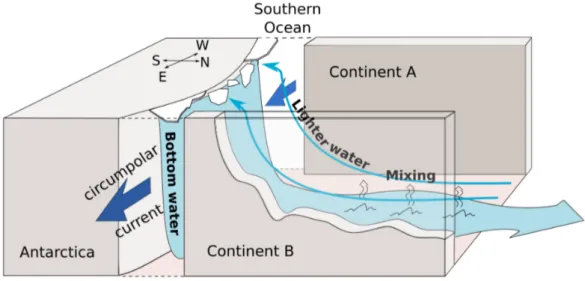
Antarctic Bottom Water

Antarctic Bottom Water is less salty (34.8 PSU), colder (T < 2◦C) and denser

(28.27 kg m−3) than the North Atlantic Deep Water.

Figure 1.5: Map of Antarctica showing the Southern Ocean and its connexions with the other basins. The Ross and Weddell Seas are two spots of Antarctic Bottom Water formation. From www.worldatlas.com

Antarctic Bottom Water is produced from the salty North Atlantic Deep Water and a portion of light fresh surface water mainly in the Weddell and Ross Seas in the Southern Ocean (see Fig. 1.5). The latter water cools by heat exchange with the cold atmosphere and during austral winter is enriched in salt by formation of sea ice and brine rejection. Cooling and enrichment in salt take place all over the winter due to the presence of polynyas in the Weddell and Ross Seas. A polynya is an open water area surrounding by sea ice, partly maintained by strong offshore katabatic winds which push seaward the newly formed sea ice (see Fig. 1.6). Without the sea ice lid, water continues to exchange heat with the atmosphere and to cool. During the same time, sea ice is continually produced in the polynya and pushed

14 1.1. Ocean water masses: description

away by the winds, enriching the water in brine rejection and thus producing the densest water mass. This dense water overflows the continental slope and fills up the Atlantic, Indian and Pacific basins below 4.5 km depth [Johnson 2008].

488 Thermohaline circulation

Cold wind from Antarctica

Cold & salty water Heat loss Coastal polynya Continental slope Sea ice Off−shore draft of sea ice Antarctic Ice Sheet Dense water overflow Entrainment Antarctic bottom water 0°C –1°C –2°C Shelf

Fig. 5.6 Formation of AABW (redrawn from Gordon, 2002).

much more complicated due to many dynamical factors, including wind stress and surface thermohaline forcing, stratification and rotation; thus, the arrows in the two-dimensional sketch (Fig. 5.3) should not be taken as being the real trajectories of water parcels.

The formation of AABW involves many complicated physical processes (Fig. 5.6), including the formation of dense and salty water within the coastal polynyas, the trans-port of this water by the gyre circulation within the coastal area, the overflow from the marginal sea to the open ocean, and the entrainment during the descent of the gravity cur-rent along the continental slope. During the descent along the slope, it entrains the water in the environment; thus, it is slightly warmed up from−2◦_{C to−1}◦_{C. Eventually, it sinks} to the bottom with a temperature of nearly 0◦_{C. Due to vigorous entrainment during the} overflow from the marginal sea to the open ocean, the total volume flux of the final product is greatly increased (Gordon, 2002). In addition, cabbeling may further increase the density of the newly formed bottom water; thus, it may play a vital role in setting the properties of the final product.

Deep convection

Another form of bottom/deep water formation in the oceans is the deep convection tak-ing place in the open ocean (Fig. 5.7). The major sites of deep convection include the northwestern Mediterranean, the Labrador Sea, and the Greenland Sea.

Figure 1.6: Sketch of a polynya and formation of Antarctic Bottom Water [Gordon 2002].

The newly formed Antarctic Bottom Water entrains and mixes with ambient Southern ocean waters to reach a maximum northward flow of about 20-30 Sv near

30◦S [Ganachaud and Wunsch 2000; Lumpkin and Speer 2007; Talley et al. 2003;

Talley 2008; 2013].

As for North Atlantic Deep Water, Antarctic Bottom Water formation is strongly influenced by the atmospheric condition around Antarctica but also by the characteristics of North Atlantic Deep Water. In a way, the formation of Antarctic Bottom Water is the result of a connexion between Arctic and Antarctic climates.

The circulation of the two main water masses and the northward return flow of surface water in the Atlantic Ocean is summarized in figure 1.7. We now turn to a full 3D description of water masses and circulation in the whole ocean.

1.1.4

A 3D ocean

The Atlantic basin is a good first step in understanding the ocean circulation, but the overall picture is more complex. The global ocean is inherently 3D and the

Overflow North Atlantic Deep Water formation Antarctic Bottom Water formation

Northward return flow

Open-ocean deep convection

Figure 1.7: Sketch of the thermohaline Atlantic ocean circulation showing the formation of dense waters in the North and the South and the presence of surface water. This sketch has been adapted from [Huang 2010].

four main basins are connected by the central and circular Southern Ocean. A rapid overview of the global ocean is given here.

Figure 1.8: Sketch of the 3D thermohaline circulation [Lumpkin and Speer 2007; Talley 2011]

Indian and Pacific oceans do not have a source of deep water as in the Atlantic ocean but their circulation is connected with the other basins through the Southern Ocean. In fact, Antarctic Bottom Water flows into the three basins, Atlantic, Indian and Pacific, where it is modified before coming back in the Southern ocean (see Fig. 1.8).

16 1.1. Ocean water masses: description

The journey of the water masses in the different basins permits the erosion of their characteristics but also to efficiently exchange nutrients, carbon and other tracers all around the world. As we will see later, the consumption of Antarctic Bottom Water in the diverse basins is an important aspect of the overturning circulation.

1.3 Various types of motion in the oceans 39

1000km 1m 10m 100m 1km 10km 100km 10000km 1Mon 1Y 10Y 100Y 1000Y 10000Y 1Hr 1Day 1Wk Barotropic tides Wind-driven gyres Internal waves Rossby waves Meso-scale eddies Kelvin waves Internal tides Thermohaline circulation Turbulence

Fig. 1.35 Various types of motion in the oceans.

Large-scale and low-frequency waves

These include Rossby waves and Kelvin waves, and they play a crucial role in the time evolution of the oceanic circulation. The major difference between these waves and the commonly encountered gravity waves is that these waves are characterized by the fact that the Earth’s rotation is their restoring force. The existence of these waves can be detected either through satellite measurements or by in situ observations.

Meso-scale eddies

These are the most energetic component of the oceanic circulation; 99 percent of the total kinetic energy in the oceans belongs to meso-scale (or synoptical scale) eddies, which can also be called geostrophic turbulence. They play an essential role in the energy cascade in the oceans. However, our knowledge about the meso-scale eddies in the oceans remains very incomplete because there are not enough data. Although satellite altimetry has provided a wealth of data for the surface expression of meso-scale eddies, observing the meso-scale

Figure 1.9: Time and spatial scales of motion in the ocean. From [Huang 2010].

The thermohaline circulation is a slow averaged circulation driven by a differential in temperature and salinity. It can be also defined as a balance of water masses in the ocean. To balance the water masses there are two processes: water mass formation and erosion. Most of the water masses are formed near the surface and sink. Furthermore, through either transformation or erosion, water mass properties are continually transformed (for example Indian Deep Water or Pacific Deep Water in figure 1.8). The thermohaline circulation is the slowest movement in the ocean with a time-scale of 100 to 10 000 years taking place all over the ocean from 100 km to 10 000 km (see Fig. 1.9). We note that this time scale only pertains to the extent and spreading of water masses. In fact, the formation of deep/bottom water happens seasonally. The long time-scale of the thermohaline circulation compared

18 1.2. Meridional overturning circulation: pushed of pulled?

1.2

Meridional overturning circulation: pushed

of pulled?

In the previous section, we described the ocean in terms of water masses but it was impossible to dissociate their origin and their future without talking about movement and circulation. But how does the ocean move?

The first thing that comes to mind is the action of the wind at the surface of the ocean. Then, from our personal experience, comes the souvenir of low tides revealing large areas suitable for catching shellfish.

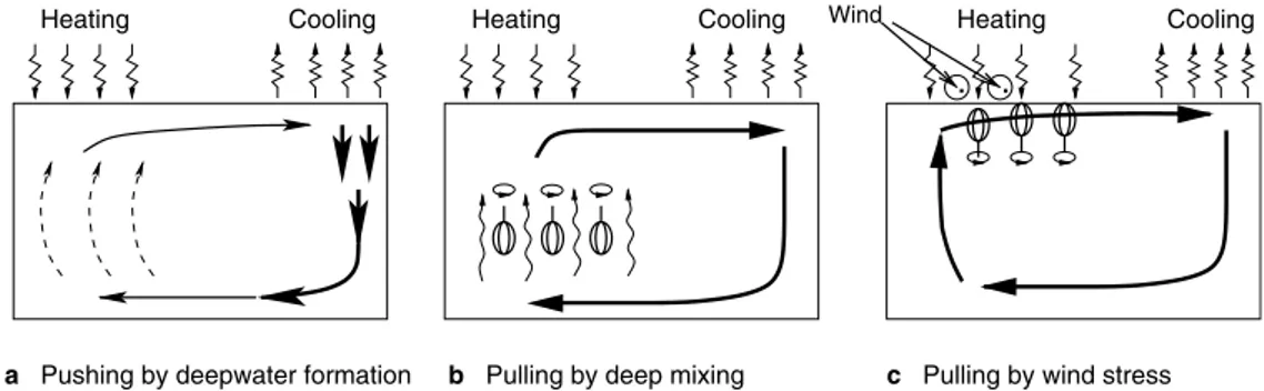
Two schools exist to explain the meridional overturning circulation: the school of pushing, for whom the main mechanism is the formation of deep water at high latitudes, and the school of pulling which considers that the overturning circulation is mainly driven by external sources of mechanical energy, such as wind stress or tidal dissipation.

1.2.1

The school of pushing: Deep water formation pushes

the deep current

5.4 Theories for the thermohaline circulation 637

Later on, this framework was modified as follows: mixing in the surface layer was replaced by diapycnal mixing at the mid depth of the ocean interior. Accordingly, the main balance in the oceanic interior is between the vertical upwelling and the downward heat diffusion, as discussed by Munk (1966). In this modified framework, there is no need for wind stress to function because the poleward flow of the surface layer is presumably driven by the pressure gradient generated by the thermohaline circulation itself. Therefore, the circulation is literally a pure thermohaline circulation. Similar to the previous framework, the circulation system consists of four segments: cold and dense water formed at high latitudes sinks to great depth; dense deep water spreads to the whole basin; deep water upwells through the base of the main thermocline and gradually warms up; surface water turns poleward and completes the cycle.

Three schools of the thermohaline circulation

Two theories, or schools, have been proposed for explaining the thermohaline circulation in the oceans. The first one, which has dominated our thinking about thermohaline circulation, postulates that thermohaline circulation is driven by deepwater formation at high latitudes, as shown in Figure 5.119a. This will be called the “school of pushing.”

The second theory postulates that a thermohaline circulation needs mechanical energy to overcome the friction; thus, the thermohaline circulation is driven by external sources of mechanical energy, such as tidal dissipation and wind stress. We will call this the “school of pulling.” The school of pulling is further separated into two sub-schools, as explained below.

1. School of pushing: Deepwater formation pushes the deep current and thus maintains the

thermohaline circulation.

In this old school of thought, the thermohaline circulation is assumed to be driven by surface thermohaline forcing, in particular the surface cooling/heating. Surface cooling pro-duces dense water that sinks to a great depth. The high-latitude ocean is filled up with cold and dense water from surface to bottom. Combining with the warm and light water in the upper ocean at low latitudes, this creates a pressure force in the abyssal ocean which causes

Heating Cooling Heating Cooling Heating Cooling

. .

Wind

b Pulling by deep mixing c Pulling by wind stress a Pushing by deepwater formation

Fig. 5.119 a–c Three schools of theory for the thermohaline circulation.

Figure 1.10: The three schools of the overturning circulation [Huang 2010].

A first glimpse of the global overturning circulation can be given by a conceptual model of the thermal overturning circulation driven by sea-surface differential heating (precipitation/evaporation can be taken into account as well without changing the results and when both effects are considered we talk about the thermohaline circulation). In this experiment, developed by Sandstrom [1908; 1916], only the thermal forcing is considered, with a cooling at one edge of the basin, representing a pole, and a heating at the other edge, representing the equator. A schematic

evolution of this experiment is given in figure 1.10a. The heating at the low latitudes expands the water and induces a sea surface uplift. Conversely, at high latitudes, water contracts and the sea surface declines. This differential in sea level creates a pressure gradient which induces a poleward movement of the surface water (in this simple experiment we do not take into account the role of Earth’s rotation). The convergence of surface water at high latitude, yields an equatorward return flow in the interior ocean. At the end, the circulation is strong only near the high latitude and confined close to the surface. The surface thermal forcing alone drives a circulation that is so weak that it is not be able to penetrate to the deep ocean. At the end, the basin has a warm layer at low latitudes, and a thick cold deep layer. In this system, the convective transfer of dense water to the bottom of the ocean is a mechanism for decreasing the potential energy; the center of mass is continually lowered. Later, Paparella and Young [2002] reformulate the discussion to show that a flow driven by buoyancy forces applied only at the surface can not generate an interior turbulence to maintain the circulation. To maintain this thermal circulation, an external source of gravitational potential energy is required. This source should be vertical mixing. Vertical mixing in a stratified fluid pushes light (heavy) water downward (upward), raising the center of mass. Vertical mixing is also called diapycnal mixing because it corresponds to a mixing across isopycnals.

1.2.2

The school of pulling by deep mixing: Deep mixing

removes cold water from the abyss

In the school of pushing, dense water piles up at the bottom. With a source of mechanical energy to sustain mixing, as described below, deep mixing transforms cold water into warm water in the deep ocean, creating space for newly formed deep water (see Fig. 1.10b and 1.11). And therefore, deep mixing pulls the thermohaline circulation [Munk and Wunsch 1998; Huang 1999].

By a simple one-dimensional scale analysis and considering that temperature, salinity and density are local functions and horizontal velocities are negligeable, Munk [1966] shows that the downward diffusion of heat or salt is balanced by the upward advection of cold water. With an upward velocity estimated from the production of dense water, he obtains a diffusivity (variable related to the mixing)

on the order of 10−4 m2s−1 needed to sustain the formation of dense water. This

20 1.2. Meridional overturning circulation: pushed of pulled?

Figure 1.11: Sketch of consumption of Antarctic Bottom Water by diapycnal mixing.

that the vertical upwelling is spatially uniform. But numerous studies point out the inhomogeneity of mixing and diverse sources of diapycnal mixing exist in the deep ocean.

a. Lee waves and internal tides

The ocean is filled with ubiquitous internal waves [Garrett and Munk 1979; Staquet and Sommeria 2002]. Internal waves are waves within interior of a stratified fluid and in the ocean can be generated by interaction of currents with topography. Idealized studies of ocean internal waves focus on two limits. The first case is a constant current impinging a seafloor topography, as mesoscale eddies, and in that case internal waves are called lee waves. The second case is a periodic current impinging a seafloor topography, for example tides, and in that case, internal waves are called internal tides. The presence of internal tides in the ocean has been detected by altimetry [Egbert and Ray 2000] and tomography records [Dushaw et al. 1995].

Several mechanisms are at the origin of the generation of lee waves: mesoscale ed-dies and large-scale circulation over topography. Garrett and Kunze [2007] estimate that 0.5 TW is supplied by large-scale currents impinging bottom topography.

An estimated value of energy input by the tides into the ocean is 3.5 TW. Internal tides are internal waves generated by a tidal current, whose frequency is given by the tide at the origin of its generation. Munk and Wunsch [1998] estimate

that 1 TW should be available to mix the abyssal ocean.

b. Geothermal heating

The geothermal heating is able to influence the circulation by heating the abyssal water from below. The heat entering in the ocean is transported into the ocean above the sea floor by molecular processes through the porous or solid seabed and by hydrothermal flux of heat carried by fluid circulating through the seabed. Nevertheless, geothermal heating is inhomogeneous in space and the estimated net energy input is only 0.05 TW [Huang 1999; Wunsch and Ferrari 2004].

c. Drag forcing on the sea floor

Drag forcing provides energy input by mechanical interaction of the mean

circulation and the eddies with the topography. It could contribute 0.1 TW

[Stammer et al. 2000].

In the 1990s, high accuracy measurements of diffusivity (variable related to

turbulent mixing) showed weak mixing over the abyssal plains (O(10−5) m2_s−1₎

and enhanced mixing up to two order of magnitude higher above rough topography [Polzin et al. 1997; Ledwell et al. 2000; Kunze et al. 2006]. Far from the Southern ocean and the other places with strong eddy kinetic energy, the principal current in the deep ocean is the barotropic tidal flow. Those two results suggest that the main source of diapycnal mixing in the deep ocean is the breaking of internal tide generated by the interaction of a tidal flow above rough topography.

1.2.3

The school of pulling by wind stress: The Southern

westerlies pull cold water from the deep ocean

Two example of wind conditions over the ocean

Winds acting on the sea surface produce direct conversion of the atmospheric kinetic energy into oceanic kinetic and potential energies. Lueck and Reid [1984] estimate a net transfer of kinetic energy from the wind field to the ocean surface-layer between 7-36 TW.

22 1.2. Meridional overturning circulation: pushed of pulled?

In this section, two examples of wind effect on the ocean circulation are developed in relation with the studies presented in this thesis.

a. Nordic Seas circulation: westerlies and easterlies

Polar cell Ferrell cell Ferrell cell Polar cell

Figure 1.12: Idealized view of the large scale flows in the atmosphere showing the easterlies linked to the polar cell and the westerlies linked to the Ferrell cell. From [Lutgens and Tarbuck 2001]

The Nordic Seas are located at the confluence of the Ferrell and polar cells (see Fig. 1.12). The Ferrel cell is associated to northwesterly winds at the surface while the polar cell has southeasterly winds at the surface. The mean wind circulation in the Nordic Seas is cyclonic [Aagaard 1970]. By friction with the water surface, water is entrained and forms a cyclonic gyre in the Nordic Seas (actually several cyclonic gyres exist in the sub-basins).

Wind stress is communicated to the ocean surface layer through viscous pro-cesses. The ocean is affected by the Coriolis acceleration and both effects (Coriolis acceleration and wind stress) permit the development of an Ekman layer. Velocity

in the Ekman layer is strongest at the sea surface (due to wind stress) and decreases exponentially downward. The Coriolis acceleration induces a velocity vector spiral with increasing depth. The transport associated with the Ekman layer is exactly perpendicular to the right (to the left) of the wind in the Northern Hemisphere (in the Southern hemisphere).

The cyclonic circulation in the Nordic Seas induces an Ekman transport toward the coasts and then an upwelling in the center of the Nordic Seas, bringing deep water to the surface. The cyclonic wind-driven circulation implies that the cooling of Atlantic water happens in the middle of the gyre while the sinking of the newly formed cold water happens along the boundaries.

b. Southern circulation: westerlies and easterlies

The circulation in the Southern Ocean is strongly linked to the winds: westerlies between 40◦S and 60◦S and easterlies south of 60◦S, closer to Antarctica. Westerlies are particularly strong due to the absence of land and entrain the water by friction (wind-stress), generating a strong Ekman flow. The Ekman flow induces an upwelling yielding a horizontal buoyancy gradient leading to a strong geostrophic current named the Antarctic Circumpolar Current (ACC). The Antarctic Circumpolar Current is affected by the seafloor like the Drake Passage, which is a semi-open boundary, allowing the flow to pass. The Antarctic Circumpolar Current is highly variable in time and space, and depends strongly on the atmospheric conditions. In Antarctica, katabatic winds blow seaward and due to the Earth’s rotation, are deviated on the left forming the easterlies. By the same processes as the westerlies, they entrain the water below and produce a westward current close to Antarctica coasts.

In the case of easterlies in the Southern Hemisphere, this implies that the Ekman transport associated to the westward current along Antarctica is southward (toward Antarctica), inducing a downwelling at the boundary. For the westerlies, the Ekman transport associated with the Antarctic Circumpolar Current is equatorward. Both

Ekman transports produce a divergence around the latitude of 50-60◦S implying

24 1.2. Meridional overturning circulation: pushed of pulled?

484 Thermohaline circulation

that, in the Pacific Basin, water of Antarctic origin with a high oxygen concentration fills up the lower part of the water column in the Southern Hemisphere. In contrast, water with very low oxygen concentration occupies the depths near 1 km in the high-latitude portion of the North Pacific Ocean, which indicates the poor ventilation of the water mass at these locations.

In addition, deep water with low oxygen concentration in the North Pacific Basin implies that there is no deepwater source in this basin. The lack of a deepwater source in the North Pacific Ocean is in great contrast to the abundant deepwater formation in the North Atlantic Ocean, and this contrast between the North Atlantic and North Pacific Oceans is one of the major features of the global thermohaline circulation under modern climate conditions.

Sources of deep/bottom water in the Atlantic Ocean

Deep water and bottom water in the Atlantic Ocean originate from marginal seas. There are primarily two sources: (1) along the edge of the Antarctic Continent, especially the Weddell Sea, and (2) Norwegian and Greenland Seas.

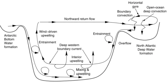
Water properties in these marginal seas and their modification during the outflow process are vitally important elements of the global thermohaline circulation. The circulation in the Atlantic Basin is a typical example, a two-dimensional sketch of which is shown in Figure 5.3. Note that the circulation is a complicated three-dimensional phenomenon; thus, the flow directions indicated in this diagram should not be interpreted as the actual flow path in the oceans. Some of the dynamical details related to this diagram will be discussed in later sections.

North Atlantic Deep Water is formed in the northern North Atlantic Ocean through two processes, including open-ocean deep convection and boundary convection associated with the horizontal gyre. Deep water formed in the Norwegian and Greenland Seas overflows the

Overflow Deep western boundary current Interior upwelling Entrainment North Atlantic Deep Water formation Boundary convection Horizontal gyre Wind−driven upwelling Entrainment Mixing & upwelling Antarctic Bottom Water formation

Northward return flow

Open-ocean deep convection

Fig. 5.3 Sketch of bottom/deep water formation and thermohaline circulation in the Atlantic Ocean.

Figure 1.13: Sketch of the diverse mechanisms behind the overturning thermohaline circulation in the Atlantic basin [Huang 2010]. The lower cell can be transposed in the Indian and pacific basins.

Effect of the wind around Antarctica on the global overturning circula-tion

The atmospheric conditions around Antarctica induce an Ekman upwelling around

the latitude of 50-60◦S. Due to this upwelling, North Atlantic Deep Water is pulled

up to the upper ocean where its properties are modified. Wind-driven upwelling is believed to represent a significant part of the globl overturning circulation and water mass transformation (see Fig. 1.10c). The wind stress energy input to the ocean is in fact larger (7-36 TW) [Lueck and Reid 1984] than the energy input due to tides (3.5 TW) [Toggweiller and Samuels 1995; Talley 2013].

1.2.4

Combination of the two schools of pulling

The total amount of mechanical energy required to sustain upwelling in the Southern ocean is estimated as 2 TW, including the estimation of tidal dissipation in the deep ocean and wind stress energy input to surface geostrophic currents [Munk and Wunsch 1998]. An emerging picture is that the upwelling is sustained by both wind stress driven Ekman transport and deep mixing [Wunsch and Ferrari 2004; Kuhlbrodt et al. 2007].

In the ocean, all the processes presented in this section exist and participate to the global overturning circulation. However, they do not contribute equally, and

wind stress and deep mixing are two keys ingredients to maintain the global overturning circulation.

26 1.3. Waves

1.3

Waves

The ocean is a stratified fluid in salinity and temperature. A perturbation in this fluid, like a rock thrown in a pond, generates waves by energy transfer from the perturbation source to the waves. Once, the waves are generated, they can propagate through the ocean and transfer energy from one point to another. Thus, the waves become a local or a remote source of energy able to generate mixing or to modify the flow.

We propose in this section to revisit three types of waves relevant to this thesis: internal waves and internal tides, Kelvin waves and topographic Rossby waves.

1.3.1

Stratified ocean: the Brunt Väisälä frequency

The action of gravity on a fluid generates a vertical pressure gradient within the fluid. For a fluid at rest, this pressure gradient is equal to the product of gravity acceleration g by the density of the fluid ρ. This equilibrium can be applied in dynamics when we consider movements essentially horizontal; more precisely it applies when the horizontal scales are much larger than the vertical scales of motion. This is the so called hydrostatic equilibrium

∂zP = −ρg, (1.1)

where the vertical axis is oriented upward, ∂z denotes partial derivative with

respect to z, and P the hydrostatic pressure. Now, if we immerse a body in a fluid submitted to gravity, the action of the hydrostatic pressure on this body corresponds to a vertical force equal to difference in weight between the body and the displaced volume; this has been demonstrated by Archimedes. In the case

of a fluid volume with density ρ1 immersed in an homogeneous fluid of density

ρ2, the Archimedes’ thrust per unit volume is

FA= (ρ2− ρ1)gz, (1.2)

where z is the unit vector in the vertical direction positive upward. In the case of the ocean, the stratification is continuous with height ρ(z), and at a given height this force will point downwards for fluid parcels heavier than the mean, and upwards for fluid parcels with density lower than the mean. This results in an equilibrium distribution of density as a function of depth with heavier, denser waters at depth. Supposing that a mean stratification ρ(z) is established, a volume dV of water with

density ρ0 will be at equilibrium at depth z0 if ρ(z0) = ρ0. Out of this position

of equilibrium, the acceleration a of the volume is

ρ0dV a = −(ρ0− ρ(z))dV gz. (1.3)

Taking the origin of the vertical axis at z = z0, we obtain

a = ∂ttz = −

g ρ0

∂zρz = −N2z. (1.4)

This equation is the equation of a harmonic oscillator at pulsation with frequency N , called the Brunt-Väisälä frequency. According to this equation, if N > 0, the fluid parcel oscillates with period 2π/N . In reality where viscous effects are present, it would oscillate with smaller and smaller amplitude, and eventually go back to its position of equilibrium due to the action of viscosity.

1.3.2

Internal gravity waves

We discussed previously the impact of mixing for the global overturning circulation. One particular type of waves is crucial to the spatial distribution of mixing, namely internal gravity waves. In this section, we introduce their main properties.

The ocean is a continuously stratified fluid and far from the thermocline and the upper ocean, the deep ocean can be considered stably and linearly stratified. Therefore a water parcel that is displaced in the vertical, for example upward, encounters water with lower density and accelerates back downward. The water parcel starts to oscillate before going back to its original position. This oscillation generates an internal gravity wave. The restoring force is the buoyancy force, which is the product of gravity and the difference in density between the displaced water parcel and the environment at the same pressure.

In the case of stratified fluid, it is common to use the Boussinesq approximation which means we consider that the fluctuations of density around the mean value are weak. In other words, we consider that the fluid has a constant density in the horizontal to leading order, with a smaller density perturbation σ: ρ(x, y, z, t) =

ρ0 + ρs(z) + σ(x, y, z, t), ρ0  ρs  σ. The vertical stratification ρs(z) is the

most important external ocean property with the Coriolis frequency f , for internal gravity waves. The stratification is characterized by the Brunt-Väsiälä frequency,

N2 _{= −}g

ρ0∂zρs. Because internal waves can have a period on the order of hours,

28 1.3. Waves

Let us now derive the dispersion relation of internal gravity waves. We consider a rotating and stratified ocean with a constant Brunt Väisälä frequency N . The unapproximated mass conservation equation is

∂tρ + u∇ρ + ρ∇ · u = Dtρ + ρ∇ · u = 0, (1.5)

where u = (u, v, w) is the velocity vector. In this equation the time scales

advectively (Dt scales in the same way as ∇ · u), then we may approximate

this equation by

∇ · u = 0. (1.6)

The motion of the fluid is governed by the Navier-Stokes equation

ρ (∂tu + u · ∇u + f k ∧ u) = −∇P + ρg + ν∆u, (1.7)

where f is the Coriolis frequency. These three equations define the dynamics of rotating and stratified fluids. To derive the dispersion relation of internal waves, we neglect the diffusive term. In general the viscous term is small compared to the other terms in the interior of the fluid, though as we will see in the next chapters it can become important for the smallest-scale internal waves. We introduce the

buoyancy perturbation b = −g(σ/ρ0). Rewriting the above equations under the

Boussinesq approximation, we obtain

∂tu + u · ∇u − f v = − 1 ρ0 ∂xp, (1.8) ∂tv + u · ∇v + f u = 1 ρ0 ∂yp, (1.9) ∂tw + u · ∇w = − 1 ρ0 ∂zp + b, (1.10) ∂tb + u · ∇b + wN2 = 0, (1.11) ∇ · u = 0, (1.12) (1.13)

where p is the nonhydrostatic pressure, and the total pressure P = phyd+ p

is composed of a part phyd in hydrostatic equilibrium with ρ0 + ρs, and a

non-hydrostatic part p. This set of equations describes the nonlinear dynamics of rotating and stratified fluids. We simplify the computation to the case of two-dimensional waves, which are the most relevant to the following chapters. We

thus work in the (x,z) plane but allowing a constant velocity v in the y direction. We also linearize the equations around a state of rest, neglecting the nonlinear terms. The above equations can then be reduced to a single equation for the

streamfunction ψ, defined as u = ∂zψ and w = −∂xψ,

∂tt∆ψ + f2∂zzψ = −N2∂xxψ. (1.14)

This equation is the linear equation of internal wave propagation in the absence of viscosity. We look for wave solutions of the form ψ0ei(k·x−ωt), where k = (k, 0, m)

is the wave vector, ω the wave frequency and x = (x, y, z). The resulting

dispersion relation is

ω2 = k

2_N2_{+ m}2_f2

k2_{+ m}2 , (1.15)

rewritten in terms of slope

k

m = ±

s

ω2_{− f}2

N2_{− ω}2 = ±tanθ. (1.16)

The angle θ can vary between 0 and π/2 and represents the angle of the wave vector k with the horizontal. There are four possible sign combinations for k and m, corresponding to the four directions of propagation for the internal wave. An important point from equation (1.16) is that the frequency of a propagative wave has to be between the Coriolis and the Brunt-Väisälä frequencies, f < ω < N .

Lee waves versus internal tides

As mentioned earlier, theoretical studies of internal waves consider the two limits of constant steady flow (lee waves) and periodic oscillating flow (internal tides). Here we described those two limits.

a. Lee waves

In the case of the lee waves, the forcing source is a steady flow with an amplitude

30 1.3. Waves U0ux− f v = − 1 ρ0 ∂xp, (1.17) U0vx+ f u = 0, (1.18) U0wx = − 1 ρ0 ∂zp + b. (1.19) U0bx+ wN2 = 0, (1.20) ux+ wz = 0. (1.21) (1.22) The set of equations can be reduced to a single equation for the vertical velocity w,

U₀2(wxx+ wzz)xx+ N2wxx+ f2wzz = 0. (1.23)

The wave solution is of the form w ∼ ei(kx+mz) and the dispersion relation

be-comes m2 = k2N 2_{− U}2 0k2 U2 0k2− f2 . (1.24)

Lee waves can radiate away if their frequency U0k is in the range f < U0k < N

so that m is real.

b. Tides and internal tides

Tides are well known since 1687 and 1775 with Newton’s [Newton 1687] theory of equilibrium tides and Laplace’s [Laplace 1775] formulation of the tidal equation. The origin of tides comes from gravitational forces exerted by the sun and the moon on Earth, including the ocean.

The presence of continents blocks the westward propagation of the tide as the Earth turns. The result is a complex pattern of tides that move around each basin. The tide in any location is unique because it is a function of the lunar and solar tidal forcing but also of the basin and coastline geometry. The relative amplitude of the tide depends on the location (see Fig. 1.14). The amplitude is zero where the cotidal lines intersect, and these points are called amphidromes.

The primary tidal frequencies observed in terms of amplitude are the semi-diurnal and diurnal. The characteristics of the tidal signal is an oscillatory movement of the whole water column, hence the name barotropic tide. It induces a back and

0") 0") I,-0 b 0 H o 0 J b w b iii b Z b Z b b 00 0 00 0 34 o_ im O c_ b 0 H o _ ,r m _ c_ w _ o _ ,rm w b z b z b b b b 35

Figure 1.14: Maps of (top) cotidal (phase) lines (in ◦) and (bottom) tidal amplitude (cm) for the semi-diurnal tide M2 Ray [1999].

forth horizontal motion of the whole water column.

Considering the semi-diurnal tide in a narrow zonal channel of uniform depth H, narrow enough that the planetary rotation may be ignored, the equations of the movement are

∂tu = −g∂x(η − ηe) (1.25)

∂tη + H∂xu = 0, (1.26)

where ηe is the equilibrium tide. In a zonal channel, this has the form

32 1.3. Waves

where ωtide is the frequency and k is the wavenumber of the semi-diurnal tide.

This represents the back and forth motion.

For the internal tides, the frequency of the waves ω is equal to the frequency

of the tide ωtide and the dispersion relation is given by (1.15).

1.3.3

Kelvin and topographic Rossby waves

Kelvin and topographic Rossby waves are believed to play an important role for the ocean transport, a hypothesis that will be further investigated and quantified in this thesis. In this section, we introduce the main properties of these waves.

In the case of a reverse 1.5-layer reduced gravity model, where we consider a thick and motionless upper layer and a thin and active bottom layer, the equations governing the dynamics (momentum equation, mass conservation equation and incompressible fluid) are

∂tu + u · ∇u + f u ∧ k = −g0∂xh + ν∆u, (1.28)

∂th + u · ∇h + h∇ · u = 0, (1.29)

∇ · u = 0, (1.30)

where u = (u, v) is the horizontal velocity, f the Coriolis frequency, g0 = g∆ρ/ρ0

the reduced gravity, h the displacement of the interface and ν the viscosity. Making the assumption that the nonlinear terms and the viscosity can be neglected, the momentum and the mass-conservation equations become

∂tu − f v = −g0∂xη, (1.31)

∂tv + f u = −g0∂yη, (1.32)

∂th + [∂x(hu) + ∂y(hv)] = 0, (1.33)

Where h(x, y, t) = H + h0(x, y) + η(x, y, t).

After calculations and using the vorticity equation (∂x(1.32) − ∂y(1.31)) and

the divergence equation (∂x(1.31) + ∂y(1.32)), we obtain

∂ ∂t h ∂ttη + f2η − ∇ · (g0h∇η) i + g0f J (η, h) = 0, (1.34)

The scale analysis of the equation gives η T3, f2η T , g0Hη L2_T , Hδg0f η L2 ,

where T is the time-scale of the waves, L the horizontal length scale, H the mean depth and Hδ is the typical size of topographic mountain heights at the horizontal scale L.

a. Kelvin waves

Kelvin waves are another type of waves whose particularity is to be "trapped" to the coastlines, which means that their amplitude is highest at the coast (y=0) and decreases exponentially seaward. Kelvin waves propagate with the coast to the right in the Northern Hemisphere (and to the left in the Southern Hemisphere).

The Kelvin wave is a high frequency wave, so the equation is dominated by the first term. The Kelvin wave is trapped to the coast so the no-normal flow boundary condition implies that v = 0 at y = 0. This result suggests that we look for a solution with v = 0 everywhere. One last thing, we consider the water depth constant and equals to H. The Kelvin wave equation is

∂ttu = c2∂xxu. (1.35)

where c = √g0_{H, the phase of shallow water waves. The solution of the}

previous equation is

u = F1(x + ct, y) + F2(x − ct, y), (1.36)

giving a surface displacement of the form

η =

s

H

g0 [−F1(x + ct, y) + F2(x − ct, y)] . (1.37)

The solution is a superposition of two waves, one (F1) travelling in the negative

x−direction, and the other in the positive x−direction. The y dependence of the wave is obtain using equation 1.32, with v = 0, which gives

∂yF1 = f √ g0_HF1, (1.38) ∂yF2 = − f √ g0_HF2, (1.39)