HAL Id: hal-02844111
https://hal.archives-ouvertes.fr/hal-02844111
Submitted on 17 Jun 2020
HAL is a multi-disciplinary open access
archive for the deposit and dissemination of
sci-entific research documents, whether they are
pub-lished or not. The documents may come from
teaching and research institutions in France or
abroad, or from public or private research centers.
L’archive ouverte pluridisciplinaire HAL, est
destinée au dépôt et à la diffusion de documents
scientifiques de niveau recherche, publiés ou non,
émanant des établissements d’enseignement et de
recherche français ou étrangers, des laboratoires
publics ou privés.
Carbon 13 Isotopes Reveal Limited Ocean Circulation
Changes Between Interglacials of the Last 800 ka
Nathaëlle Bouttes, Natalia Vazquez Riveiros, Aline Govin, Didier
Swingedouw, Maria F. Sanchez-Goni, Xavier Crosta, Didier M. Roche
To cite this version:
Nathaëlle Bouttes, Natalia Vazquez Riveiros, Aline Govin, Didier Swingedouw, Maria F.
Sanchez-Goni, et al.. Carbon 13 Isotopes Reveal Limited Ocean Circulation Changes Between Interglacials of
the Last 800 ka. Paleoceanography and Paleoclimatology, American Geophysical Union, 2020, 35 (5),
pp.e2019PA003776. �10.1029/2019PA003776�. �hal-02844111�
N. Bouttes1,2 , N. Vazquez Riveiros3 , A. Govin1 , D. Swingedouw2, M. F. Sanchez‐Goni2,4 , X. Crosta2, and D. M. Roche1,5
1Laboratoire des Sciences du Climat et de l'Environnement, LSCE/IPSL, CEA‐CNRS‐UVSQ, Université Paris‐Saclay,
Gif‐sur‐Yvette, France,2Université de Bordeaux EPOC, UMR 5805, Pessac, France,3IFREMER, Unité de Géosciences
Marines, Plouzané, France,4Ecole Pratique des Hautes Etudes (EPHE, PSL University), Pessac, France,5Earth and Climate Cluster, Faculty of Science, Vrije Universiteit Amsterdam, Amsterdam, The Netherlands
Abstract
Ice core data have shown that atmospheric CO2concentrations during interglacials were lowerbefore the Mid‐Brunhes Event (MBE, ~430 ka), than after the MBE by around 30 ppm. To explain such a difference, it has been hypothesized that increased bottom water formation around Antarctica or reduced Atlantic Meridional Overturning Circulation (AMOC) could have led to greater oceanic carbon storage before the MBE, resulting in less carbon in the atmosphere. However, only few data on possible changes in interglacial ocean circulation across the MBE have been compiled, hampering model‐data comparison. Here we present a new global compilation of benthic foraminifera carbon isotopic (δ13C) records from 31 marine sediment cores covering the last 800 ka, with the aim of evaluating possible changes of interglacial ocean circulation across the MBE. We show that a small systematic difference between pre‐ and post‐MBE interglacialδ13C is observed. In pre‐MBE interglacials, northern source waters tend to have slightly higherδ13C values and penetrate deeper, which could be linked to an increased northern sourced water formation or a decreased southern sourced water formation. Numerical model simulations tend to support the role of abyssal water formation around Antarctica: Decreased convection there associated with increased sinking of dense water along the continental slopes results in increasedδ13C values in the Atlantic in agreement with pre‐MBE interglacial data. It also yields reduced atmospheric CO2as in pre‐MBE records,
despite a smaller simulated amplitude change compared to data, highlighting the need for other processes to explain the MBE transition.
1. Introduction
Measures of air trapped in ice cores have shown that atmospheric CO2concentration during interglacials
were lower before the Mid‐Brunhes Event (MBE, around 430 ka), with values of 241 ± 6 ppmv, than after the MBE, when interglacial CO2concentrations were 273 ± 7 ppmv (Lüthi et al., 2008; Bereiter et al., 2015;
Figure 1). The ocean is a major carbon reservoir, currently holding around 50 times the carbon in the atmo-sphere. The lithosphere contains even more carbon, but the associated residence time of carbon is too large to be the prime cause of carbon changes on millennial times scales, while the residence time of carbon in the ocean is small enough to make the ocean a potential driver of carbon changes during glacial‐interglacial cycles. Changes in ocean circulation can modify the amount of carbon stored in the ocean, and an increase of ocean carbon storage would result in a lowering of atmospheric CO2concentration.
So far, only one box model has explored the possibility of increased oceanic carbon storage due to ocean cir-culation changes during interglacials before the MBE. Köhler and Fischer (2006) have used a simple box model allowing them to prescribe the oceanic circulation. They have shown in their simulations that the lower CO2concentration of the pre‐MBE interglacials can be obtained mainly with lower sea‐surface
tem-peratures in the Southern Ocean and a weaker Atlantic meridional overturning circulation (AMOC). A more complex model, the LOVECLIM intermediate complexity model, has been used to evaluate changes of ocean circulation in response to changes in insolation forcing during interglacials (Yin, 2013). Contrary to the box model, the ocean circulation in LOVECLIM is computed instead of being prescribed. LOVECLIM was used to run nine simulations with the orbital configurations of nine interglacials, resulting in different ocean circulations changes. In these simulations, Antarctic bottom water formation in the Southern Ocean was increased during interglacials preceding the MBE compared to the more recent
©2020. American Geophysical Union. All Rights Reserved.
Key Points:
• Sediment core data show a systematic oceanicδ13C difference between interglacials before and after the Mid‐Brunhes Event (MBE) • Model simulations show that it can
be partly due to ocean circulation changes
• But ocean circulation change can only account for 1/3rd of the measured atmospheric CO2 change between interglacials over the MBE
Supporting Information: • Supporting Information S1 Correspondence to: N. Bouttes, nathaelle.bouttes@lsce.ipsl.fr Citation:
Bouttes, N., Riveiros, N. V., Govin, A., Swingedouw, D., Sanchez‐Goni, M. F., Crosta, X., & Roche, D. M. (2020). Carbon 13 Isotopes Reveal Limited Ocean Circulation Changes Between Interglacials of the Last 800 ka. Paleoceanography and
Paleoclimatology, 35, e2019PA003776. https://doi.org/10.1029/2019PA003776
Received 30 SEP 2019 Accepted 26 MAR 2020
interglacials. The carbon cycle was not simulated, but it was suggested that such circulation changes should impact the carbon cycle.
However, with another version of this model, iLOVECLIM, which includes an interactive carbon cycle, Bouttes et al. (2018) have shown that the increased overturning in the Southern Ocean that is simulated is not sufficient to explain the lower pre‐MBE CO2values, as the ocean circulation changes are too small to
sufficiently increase oceanic carbon storage. It results from these simulations that either this climate model is not able to simulate large enough ocean circulation changes, possibly because of misrepresented pro-cesses, or that ocean circulation changes were small and other mechanisms were responsible for the lower pre‐MBE atmospheric CO2.
A few available proxies document past ocean ventilation changes. In particular, the ratio of13C over12C of dissolved inorganic carbon, the so‐called δ13C, is often used as an indicator of ocean circulation patterns since ocean circulation is one of the main factors determining oceanic δ13C distribution (Duplessy et al., 1988). The water masses are formed at the surface with a characteristicδ13C value depending on frac-tionation from air‐sea exchange and biological activity, which enriches organic carbon in12C and the sur-rounding water in13C. The water masses with relatively highδ13C values then sink to depth and during their transport they are progressively enriched in 13C‐depleted carbon released from remineralization, which lowers theirδ13C. The longer the water is transported and isolated from the atmosphere before com-ing back to the surface, the lower itsδ13C becomes. Hence, all other factors staying constant, high values of bottom waterδ13C are an indication of high ventilation, while low values ofδ13C indicate that the water mass is“old”; that is, it has not been in contact with the atmosphere for a long time.
In the modern ocean, North Atlantic Deep Water (NADW) formed in the Nordic and Labrador seas has high δ13C values (generally higher than 1.0‰), while Antarctic Bottom Water (AABW) formed in the Southern
Ocean has lower values (generally lower than 0.5‰; Schmittner et al., 2013; Kroopnick, 1985). In the past, δ13
C of epibenthic foraminifera (e.g., Cibicides genus) has been used to characterize changes in bottom water δ13C, and thus, past ocean circulation changes at different timescales. As an example, the Last Glacial
Maximum (around 21,000 years ago) exhibits large differences in theδ13C distribution compared to the mod-ern ocean (Curry & Oppo, 2005; Hesse et al., 2011; Marchal & Curry, 2008; Oliver et al., 2010). In particular, the glacial abyssal waters in the Southern Ocean were characterized by very lowδ13C values below−0.4‰ (compared to higher than 0.2‰ for the modern) while surface waters had high δ13
C values, indicating enhanced stratification of the water column (e.g., Curry et al., 1988).
Despite the decreasing number of data when going back in time, there are a number of sediment cores with relatively well‐resolved benthic δ13C records spanning the last 800,000 years (Past Interglacials Working Group of PAGES, 2016). For example, Lisiecki (2010) combined 13 sediment cores in three stacks to study the evolution of Pacific deep water as a mix of North and South Atlantic water. Since then, more data have become available.
To better understand interglacial oceanic circulation changes during the last 800,000 years, we present here a new compilation of 31δ13C data from sediment cores covering the Atlantic, Pacific, and Indian oceans, and combine this data compilation with simulations including δ13C changes obtained with intermediate
Figure 1. Atmospheric CO2(ppm), data from Bereiter et al. (2015). The purple bars indicate the time of the CO2used for the simulations, taken as the time of the insolation maximum preceding the interglacialδ18O peak identified in the LRO4δ18O stack (Lisiecki & Raymo, 2005).
10.1029/2019PA003776
Paleoceanography and Paleoclimatology
complexity model runs for the last nine interglacials. We use observational data and model simulations to evaluate the possibility of systematic changes of ocean circulation during the pre‐MBE interglacials compared to post‐MBE interglacials. In particular, we focus on the Atlantic where the variations in oceanic circulation during glacial‐interglacial cycles indicate that changes of carbon storage could have potentially occurred. This is also the region where most data lie.
2. Methods
2.1. δ13C Data Compilation
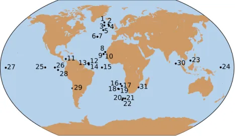
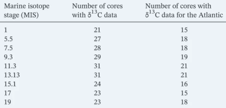
We have compiledδ13C data from the benthic foraminifera genus Cibicidoides sp. from existing sediment cores for the last 800,000 years (Table 1, Figure 2). We have selected sediment cores for which oxygen and carbon stable isotopes measured on benthic foraminifera are available for at least one interglacial period before and one after the MBE, for example, at least for MIS11 and MIS13 (core number 6; Figures 3 and 4). In total, we have compiled 31 sediment cores (Table 1, Figure 2). Among them, a subset of eight sediment cores has data for all the considered interglacials of the last 800,000 years (Figures 3 and 4). Most cores are situated in the Atlantic (22 cores), a few in the equatorial Pacific (seven cores), and two in the Indian Ocean (Figure 2). Finally, there are at least 21 cores from all ocean basins withδ13C data covering each inter-glacial and 15 cores from the Atlantic Ocean only (Table 2).
The original age model is used when available and in agreement with the LR04 chronology (Lisiecki & Raymo, 2005). Alternatively, the age model of the last 800 ka is obtained or revised by aligning the benthic δ18O records to the LR04 benthic δ18O stack (Lisiecki & Raymo, 2005) with the AnalySeries software
Table 1
Marine Sediment Cores Considered in this Study and Corresponding Age Model
Core nb Core name Latitude Longitude Depth (m) Reference Age model
1 ODP 983 60.00 −24 1,983.00 Raymo et al., 2004 New with LR04 tuning 2 ODP 982 57.51 −15.88 1,145.00 Venz et al., 1999 New with LR04 tuning 3 DSDP 552 56.05 −23.24 2,301.00 Shackleton and Hall, 1984 New with LR04 tuning 4 ODP 980‐981 55.48 −14.70 2,168.00 Oppo et al., 1998; McManus et al., 1999;
Flower et al., 2000
Original + improved for MIS11, MIS13 5 ODP U1308 49.88 −24.24 3,883.00 Hodell et al., 2008 Original
6 ODP U1313 41.00 −32.96 3,426.00 Voelker et al., 2010; Ferretti et al., 2010 Original
7 DSDP 607 41.00 −32.96 3,427.00 Raymo et al., 1989; Ruddiman et al., 1989 New with LR04 tuning 8 ODP 658 20.75 −18.58 2,271.00 Sarthein and Tiedermann, 1989 New with LR04 tuning 9 MD03‐2705 18.10 −21.15 3,085.00 Malaizé et al., 2012 Original
10 ODP 659 18.08 −21.03 2,271.00 Sarnthein and Tiedemann, 1989 New with LR04 tuning 11 DSDP 502 11.49 −79.38 3,051.00 deMenocal et al., 1992 New with LR04 tuning 12 ODP 929 5.98 −43.74 4,356.00 Bickert et al., 1997 New with LR04 tuning 13 ODP 927 5.46 −44.48 3,315.00 Bickert et al., 1997 New with LR04 tuning 14 ODP 925 4.20 −43.49 3,041.00 Bickert et al., 1997 New with LR04 tuning
15 ODP 664 0.11 −23.23 3,806.00 Raymo et al., 1997 Original + improved for 400–550 ka 16 GeoB 1034‐3 −21.74 5.42 3,731.00 Bickert, 1992 Original + improved for MIS5,
MIS11, MIS13, MIS15, MIS17 17 GeoB 1211 −24.48 7.53 4,084.00 Bickert, 1992; Bickert and Wefer, 1996 New with LR04 tuning
18 ODP 1267 −28.10 1.71 4,355.00 Bell et al., 2014 Original
19 ODP 1264 −28.53 2.85 2,504.00 Bell et al., 2014 Original
20 ODP 1089 −40.94 9.89 4,620.50 Hodell et al., 2003 Original + improved for MIS9, MIS13, MIS15 21 ODP 1088 −41.14 13.56 2,081.20 Hodell et al., 2003 Original + improved for MIS9, MIS13, MIS15 22 ODP 1090 −42.91 8.90 3,701.60 Hodell et al., 2003; Venz & Hodell, 2002 Original + improved for MIS15, MIS17 23 ODP 1143 9.36 113.29 2,771.00 Wang et al., 2004; Cheng et al., 2004 New with LR04 tuning
24 ODP 806B 0.32 159.36 2,519.90 Berger et al., 1993 New with LR04 tuning
25 ODP 849 0.18 −110.52 3,839.00 Mix et al., 1995 Original + redone for MIS15, MIS17 26 RC13‐110 0.10 −95.65 3,231.00 Mix et al., 1991 New with LR04 tuning
27 RC13‐229 −0.17 −171.2 5,316.00 Oppo et al., 1990 Original 28 ODP 846 −3.10 −90.82 3,296.00 Mix et al., 1995; Raymo et al., 2004 Original 29 GeoB 15016 −27.49 −71.13 956.00 Martínez‐Méndez et al., 2013 Original
30 ODP 758 5.38 90.36 2,935.00 Chen et al., 1995 New with LR04 tuning 31 MD96‐2048 −26.17 34.02 660.00 Caley, unpublished results; Caley et al., 2011 Original
(Paillard et al., 1996). In case of oxygen isotopic measurements on multiple foraminifera species, we used all available benthic species, and added 0.64‰ to Cibicidoides δ18O values to match Uvigerina sp. values (Shackleton & Opdyke, 1973). Visual control of theδ18O evolution for each core ensures that there is no large shift between records (Figure 2).
The dates that define the nine interglacials (Table 3) are chosen here by selecting the interglacial δ18O peaks in LR04 (Lisiecki & Raymo, 2005), in order to correspond to the same interglacial periods selected by Yin and Berger (2010, 2012), and to compare data with existing model simulations (Bouttes et al., 2018) for which boundary conditions are taken at the insolation maxima just preceding theδ18O peaks (Table 3). Theδ13C data values for each of the nine interglacials are averaged over an interval chosen using the Southern Component Water (SCW)δ13C stack from Lisiecki (2010), which clearly displays glacial‐interglacial cycles. Intervals are defined to cover the interglacial δ13C plateau displayed by theδ13C stack just after each of the interglacials selected with theδ18O peaks. We take the plateau after theδ18O peaks to account for the delays in response of ocean and vegetation changes to insolation evolution. These time intervals are given in Table 3 and shown on Figures 3 and 4 with gray shading.
We focus on the Atlantic Ocean where most data lie (Figure 3), and where previous hypothesis of circulation changes (weaker AMOC, stronger AABW formation) have been put forward (Köhler & Fischer, 2006; Yin, 2013). We have interpolated the Atlantic data using the Ocean Data View software (ODV; Schlitzer, 2017) with the DIVA (Data‐Interpolating Variational Analysis) gridding.
2.2. Model Simulations
We compare the data compilation to model simulations previously run with the iLOVECLIM model (Bouttes et al., 2018). iLOVECLIM is an evolution of the LOVECLIM version 1.2 intermediate complexity model (Goosse et al., 2010). It has the same atmosphere and ocean modules, which are respectively on a T21 spectral grid truncation (~5.6° in latitude/longitude in the physical space) with three vertical layers, and on a 3° by 3° horizontal grid with 20 vertical levels. iLOVECLIM includes a terrestrial biosphere module called VECODE (Brovkin et al., 1997) and an ocean biogeochemical module (Bouttes et al., 2015). The latter simulates the ocean carbon isotope distribution, which can thus be directly compared to benthic foramini-feraδ13C data. The simulations were run by prescribing the orbital configurations (Berger, 1978), atmo-spheric CO2(Bereiter et al., 2015) and modeled ice sheets (Ganopolski & Calov, 2011) at the time of the
maximum insolation just preceding theδ18O peaks (Table 3). The simulations have already been analyzed in terms of carbon storage and atmospheric CO2(Bouttes et al., 2018), but not in terms of oceanicδ13C
dis-tribution. Note that the model includes two variables corresponding to atmospheric CO2. Thefirst one is for
the radiative code and is prescribed based on data (Bereiter et al., 2015). The second one is a prognostic CO2
computed in the carbon cycle module due to the exchange of carbon between the ocean, atmosphere and terrestrial biosphere.
Figure 2. Map of selected marine sediment core locations. The numbers corresponding to each core are documented in Table 1.
10.1029/2019PA003776
Paleoceanography and Paleoclimatology
In addition, we have performed three new sensitivity experiments to test the impact of various ocean circu-lation configurations on δ13
C distribution and evaluate the possibility of missing processes that may affect the circulation. We chose to impose MIS17 boundary conditions as an example of a pre‐MBE interglacial, because data indicate that it is a particularly interesting interglacial in terms of changes of deep water forma-tion sites in the Nordic seas (Poirier & Billups, 2014; Wright & Flower, 2002). To evaluate the impact of
Figure 3.δ18O (permil) evolution for each marine sediment core (Table 1) over the last 800,000 years. Gray shading indicate theδ13C date intervals, the dotted lines indicate the dates for the orbital configurations and CO2used for the
changes in surface freshwater forcing in the North Atlantic, which is poorly constrained and very complex to properly simulate due to different ice sheet configuration that may have affected the hydrological cycle, we add a positive fresh waterflux of 0.2 Sv in the North Atlantic (“Ruddiman belt,” roughly between 30°N and 60°N), following Roche et al. (2010), in simulation“MIS17 hosing 0.2 Sv.” In simulation “MIS17 hosing −0.2 Sv”, we similarly add a negative fresh water flux of −0.2 Sv in the North Atlantic. Finally, in simulation “MIS17 brines,” we activate the sinking of dense water along the continental slopes to the abyss around
Figure 4.δ13C (permil) evolution for each marine sediment core (Table 1) over the last 800,000 years. Gray shading indicate theδ13C date intervals, the dotted lines indicate the dates for the orbital configurations and CO2used for the
model simulations. The numbers to the left refer to the core numbers (Table 1, Figure 2).
10.1029/2019PA003776
Paleoceanography and Paleoclimatology
Antarctica with a“frac” parameter (fraction of the salt rejected by sea ice sinking to the bottom of the ocean) set to 0.4 following Bouttes et al. (2010). With this parameterization, a fraction (frac) of the salt (and all other vari-ables) that is rejected during the formation of sea ice, and is by default expelled in the surface cell, is instead directly transferred to the bottom cell to mimic the effect of the sinking of very dense water along the conti-nental slope.
3. Results and Discussion
3.1. δ13C Data Distributions
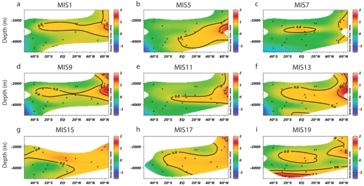
In the obtained data compilation, most interglacial Atlanticδ13C distri-butions show similar features (Figures 5 and S1 in the supporting infor-mation) that appear as characteristic of an interglacial. They exhibit high δ13C values for NADW, generally decreasing from around 1.2‰ in the northern surface ocean where the dense water is formed, down to around 0.8‰ in the ocean interior where NADW penetrates. We observe lowerδ13C values, generally around 0‰, in the abyssal South Atlantic, that we attribute to AABW. Nonetheless, the interglacials show a variety of distributions with some differences among them. The most striking features are the high δ13C values, especially in the North Atlantic, for MIS11 and MIS13, as well as MIS1. On the opposite, MIS7, MIS9, and MIS19 display lowδ13C values for NADW. Little difference seems to take place in the Southern Ocean, but the number of sediment cores in this region is small. In the Pacific and Indian oceans, the number of cores is very restrained with seven cores in the Pacific and only two in the Indian. We use a subset of the Pacific sediment cores as detailed in section 3.3, but the Indian data are not used in this study. We still display theδ13C values in these basins on Figure S2.
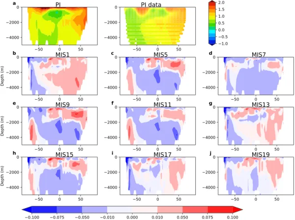
3.2. Simulatedδ13C Distributions
Figure 6 shows the preindustrialδ13C distribution in the Atlantic Ocean for the model and observations, and the difference between each interglacial simulation and the pre‐industrial simulation. Compared to the observations, the model reproduces the main characteristics of theδ13C distribution in the Atlantic including the higher values for NADW and lower values for AABW (Bouttes et al., 2018). The model simulations for the nine interglacials result in small δ13C changes among interglacials (Figure 6). All simulations result in δ13C distributions similar to the pre‐industrial, with higher NADW values and lower AABW values. Some interglacials, such as MIS1, MIS13, MIS17, and MIS19, display slightly higher values in the North Atlantic around 3,000‐m depth, but the magnitude of the differences is very small (around 0.05‰).
3.3. Correcting for Long‐Term Changes in Global Mean Ocean δ13C
The high values for MIS11, and even higher values for MIS13, compared to lower values for the other interglacials (Figure 5), could be linked to the long‐term changes of the carbon cycle that have previously been reported in δ13C records. Indeed, some sediment cores show long‐time oscillations related to a ~400 ka cycle that have been observed from the Eocene to the Quaternary (Bassinot et al., 1994; Billups et al., 2004; Hoogakker et al., 2006; Pälike et al., 2006; Sexton et al., 2011; Tian et al., 2018; Wang et al., 2010). Various hypotheses have been proposed to explain these 400 ka oscillations. The monsoon is linked to changes in eccentricity as low latitude precipitation depends on precessional for-cing and can be modulated by eccentricity. Monsoon seems to play an important role in driving carbon cycle changes, especially via organic car-bon burial on continental shelves that depends on river discharge. These changes could also be related to modifications in marine global productiv-ity or rain ratio (ratio of calcium carbonate to organic carbon sinking as particulate matter to the deep ocean) (Paillard, 2017; Paillard &
Table 2
Number of Cores Withδ13C Data for Each Considered Interglacial Marine isotope
stage (MIS)
Number of cores withδ13C data
Number of cores with δ13C data for the Atlantic
1 21 15 5.5 27 18 7.5 28 18 9.3 29 19 11.3 31 21 13.13 31 21 15.1 24 16 17 23 15 19 23 18 Table 3
Marine Isotope Stage (MIS) and Dates Used for Data Averages and Model Simulations
Marine isotope stage (MIS)
Date of orbital configuration and CO2(ka) (used for
simulations) Date ofδ18O peak (ka) Dates forδ13C interval (ka) 1 12 6 0–6 5.5 127 123 120–126 7.5 242 239 234–240 9.3 334 329 310–328 11.3 409 405 400–418 13.13 506 501 486–518 15.1 579 575 570–575 17 693 696 694–704 19 788 780 772–778
Figure 5.δ13C distribution (permil) in the Atlantic Ocean from sediment cores using the Ocean Data View software for the nine considered interglacials. The black dots indicate the position of the sediments cores with data covering the considered interglacials.
Figure 6.δ13C distribution (permil) in the Atlantic Ocean from model simulations using iLOVECLIM (a) absoluteδ13C values for the preindustrial simulation compared to PI reconstruction (Eide et al., 2017), (b–j) δ13C anomalies with respect to the PI for the nine interglacials.
10.1029/2019PA003776
Paleoceanography and Paleoclimatology
Donnadieu, 2014; Russon et al., 2010). In this study, we focus on ocean cir-culation both with data and model. In the model used, there is no net exchange with the lithosphere (weathering and burial of organic matter); hence, the processes responsible for the 400 ka cycle are not accounted for and these long‐term changes cannot be simulated.
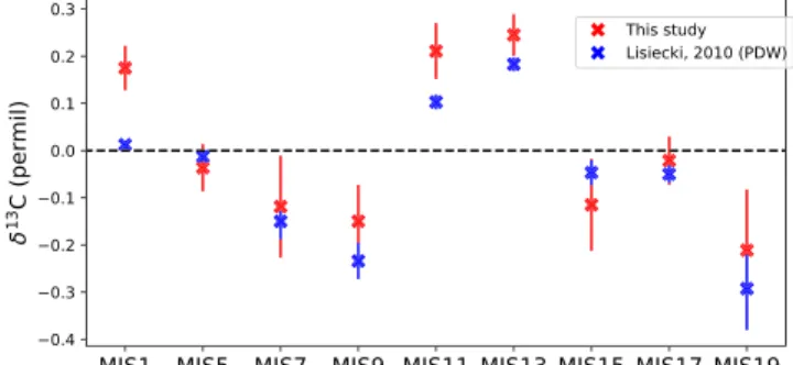
To eliminate this long 400‐ka periodicity from the records in an effort to retain only the interglacial characteristics, we hypothesize that limited glacial‐interglacial circulation changes occurred in the deep equatorial Pacific and thus that the epibenthic δ13C of deep equatorial Pacific cores records past changes in global mean oceanδ13C. This hypothesis is sup-ported by the observation that the meanδ13C change of deep Pacific cores (2,500‐ to 4,000‐m water depth) between the Last Glacial Maximum (LGM) and the Holocene is indistinguishable from the LGM‐Holocene global mean oceanδ13C change (Duplessy et al., 1988). Hence, we assume that the mean deep equatorial Pacific δ13C signal reflects past variations in global mean oceanδ13C and is mainly driven by the long term 400 ka change in carbon cycle. Therefore, we remove from all records the mean deep equatorial Pacific signal, taken as the average of epibenthic δ13C values from equatorial Pacific cores below 2,500 m and above 4,000 m (cores 24, 25, 26, and 28 in Figure 3; cf. Figure 7). We compare our mean deep equatorial Pacific signal to the Pacific Deep Water δ13
C stack calculated by Lisiecki (2010) with a slightly different set of cores and verify that the variations of global mean oceanδ13C across interglacials are the same. We observe in particular higher values during MIS11 and MIS13 compared to other interglacials (excluding MIS1). In the calculations that follows, using the meanδ13C Pacific signals from Lisiecki (2010) (not shown) yields similar results as with our Pacific δ13C means (Figure 7). There are slight differences between our meanδ13C Pacific signal and the one from Lisiecki (2010) for several interglacial periods (e.g., MIS1, MIS9, MIS11, MIS13, and MIS19), due to the fact that the selected cores differ. Our mean Equatorial Pacific signal is derived from four cores (ODP 806B [24], ODP 849 [25], RC13‐110 [26], and ODP 846 [28]), while it is calculated from four slightly different cores (ODP 806B, ODP 849, ODP 846, and ODP 677) in the study by Lisiecki (2010). Removing core RC13‐110 from our mean Pacific δ13C signal leads to only minor changes (not shown) and do not explain the higher mean δ13C values observed for several interglacials in our study compared to that of Lisiecki (2010). Hence the
dif-ference comes from ODP 677, used in the Lisiecki's Pacific deep‐water stack and not in ours. Here we decided to only keepδ13C data from the epifaunal Cibicidoides genus, which better reflect the δ13C value of deep waters (Curry et al., 1988; Duplessy et al., 1988). Because most stable isotope measurements in core ODP 677 have been performed on the endofaunal Uvigerina genus (Shackleton & Hall, 1989), we did not include this core in our study. The originalδ13C values measured on the Uvigerina genus have been cor-rected to Cibicidoides equivalentδ13C values (Shackleton & Hall, 1989; Lisiecki, 2010). We think that the cor-rection factor applied on ODP 677 Uvigerinaδ13C values did not sufficiently correct these values, which remained low compared to other Pacific δ13C records measured on the Cibicidoides genus (seefig. 1b in Lisiecki, 2010). These generally decreased benthicδ13C values in core ODP 677 likely explain why the mean Pacific δ13C signal appears to be lower for several interglacials in the study by Lisiecki (2010) compared to our study (Figure 7).
As expected, removing the mean equatorial Pacific signal globally increases the initially low δ13C values of MIS7, MIS9, MIS19, and globally decreases the initially highδ13C values of MIS11 and MIS13 (Figure 8). After correcting for the long termδ13C evolution, theδ13C distributions for each of the nine interglacials (Figure 8) remain relatively similar with higher δ13C values for NADW and lower values for AABW. MIS11 now resembles more the rest of the post‐MBE interglacials (i.e., MIS1, MIS5, MIS7, and MIS9), with a thin tongue of NADW withδ13C values between 0.8‰ and 1.2‰ extending into the Southern Hemisphere at ~3,000 m deep. Most pre‐MBE interglacials (except MIS19) still seem to display larger areas, extending deeper, ofδ13C values higher than 0.8‰ compared to post‐MBE interglacials (Figure 8). This increase of δ13C values for the pre‐MBE interglacials, especially in the North Atlantic, is in agreement with the
recon-struction from Barth et al. (2018) with a smaller number of cores.
Figure 7. Pacific mean δ13C values (permil) for each interglacial using sediment cores 24, 25, 26, and 28 (this study), and as computed in Lisiecki (2010) to characterize Pacific Deep Water (PDW). The standard error is indicated by the vertical bars. Theδ13C means (this study and Lisiecki, 2010) are computed using theδ13C time intervals given in Table 3.
3.4. Are there Systematic Atlanticδ13C Differences Before and After the MBE?
To evaluate whether there is a systematic difference between pre‐ and post‐MBE interglacial Atlantic δ13
C distributions, we havefirst computed the difference between the average of pre‐MBE and post‐MBE δ13C distributions at each core site (Figure 9a). We have only applied this calculation to the subset ofδ13C records that present at least three interglacials before and three after the MBE. At most core locations, theδ13C values are higher in the pre‐MBE interglacials than the post‐MBE interglacials. However, the significance is low and only six cores exhibit significant differences at the 90% level (two sided t test) (Figure 9b), due to the high variations inδ13C mean values among pre‐ and post‐MBE interglacials.
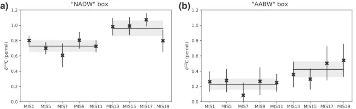
To characterize more specifically the changes in NADW and AABW, we have also computed mean δ13C in boxes representing NADW and AABW for each interglacial. For NADW, we consider the average of
Figure 8.δ13C distribution (permil) in the Atlantic Ocean from sediment cores using the Ocean Data View software for the nine considered interglacials with the Pacific signal removed (using the mean values from this study indicated on Figure 7).
Figure 9. (a) Composite ofδ13C values (permil) in the Atlantic for the interglacials (after removing the mean Pacific signal), computed as the difference between the average of pre‐MBE interglacial (MIS13, MIS15, MIS17, MIS19) δ13C and the average of the post‐MBE interglacial (MIS1, MIS5, MIS7, MIS9, MIS11) δ13C. (b) Significant cores at the 0.1 level are indicated in black, nonsignificant cores in white. (c) Propagated error for each sediment core using the quadratic sum
of standard errors for each time periods.
10.1029/2019PA003776
Paleoceanography and Paleoclimatology
mid (between 1,000 and 4,000 m) North Atlanticδ13C value and for AABW the average of abyssal (below 3,500 m) South Atlantic δ13C values (see boxes on Figure 9a). Both δ13C means for the upper North Atlantic (“NADW” box) and abyssal South Atlantic (“AABW” box) show systematic changes across the MBE (Figure 10). Although changes are small, around 0.2‰, they generally show higher values in pre‐MBE interglacials compared to post‐MBE interglacials. This could possibly indicate a small increase in ocean ventilation in the Atlantic, although the link betweenδ13C and ocean circulation changes is not straightforward (Menviel et al., 2015). We test this possibility with model simulations as described in section 3.6.
3.5. Are the Pre‐MBE δ13
C Values Comparable to a Weak LGM State?
The LGM is the best‐known example of a very different Atlantic δ13C distribution that could be due to a more stratified ocean. To evaluate whether the pre‐MBE interglacial ocean circulation could resemble a glacial one, we compare theδ13C in the 9 interglacials to the LGM values.
Using the“NADW” and “AABW” boxes previously defined, we can compute the δ13C gradient between the mean of these two boxes and compare the gradient of pre‐and post‐MBE interglacials to the LGM and Holocene, using the eastern Atlanticδ13C data from LGM and Holocene of Marchal and Curry (2008)), since this is where most of our data lie.
The LGMδ13C distribution is characterized by a much largerδ13C gradient between the“NADW” box and “AABW” box compared to the Holocene (Figure 11). The LGM gradient is 1.1‰, around 0.7‰ higher than the Holocene one at 0.4‰. This δ13C gradient reflects the greater stratifi-cation of the glacial ocean and is taken as an indistratifi-cation of the different oceanic circulation in glacial conditions (Curry & Oppo, 2005). We now test whether the pre‐MBE interglacials could be more similar to the LGM than to the Holocene.
The δ13C gradients for the nine interglacials, ranging from 0.25‰ to 0.70‰, are all closer to the Holocene values than to the LGM values. None of the interglacialδ13C distributions displays the glacial features of a more stratified ocean with lower values in the deeper ocean and higher values in the upper ocean, as observed for the LGM 21,000 years ago (Curry & Oppo, 2005; Marchal & Curry, 2008). If the MIS19 gradient is removed, the pre‐MBE interglacial values are slightly higher than the post‐MBE interglacial values. Yet, the abyssal Southern Ocean δ13C values reach very low values at the LGM compared to the Holocene, while the pre‐MBE interglacials are characterized by higher δ13C values in this region compared to the post‐MBE interglacials. Hence, the pre‐MBE interglacialδ13C distributions are radically different from the LGM one.
Figure 10. Meanδ13C (permil) computed in the“NADW” and “AABW” boxes defined on Figure 9, using the δ13C corrected with the mean equatorial Pacific signal (Figure 7). The error bars give the propagated error using the quadratic sum of standard errors for the NADW and deep equatorial Pacific signal for (a) and AABW and deep equatorial Pacific signals in (b).
Figure 11.δ13C gradient (permil) between the mean δ13C in the mid‐North Atlantic (“NADW” box) and the mean δ13C in the lower South Atlantic (“AABW” box). Holocene and LGM δ13C data are for the eastern Atlantic (Marchal & Curry, 2008). The error bars indicate the standard error for each time period.
3.6. Can the Recorded Changes ofδ13C Be Explained by Changes in Oceanic Circulation?
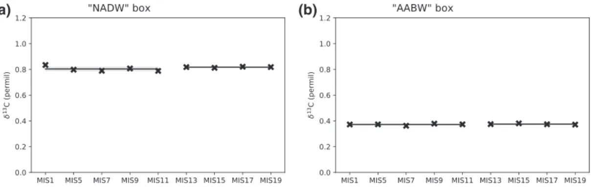
To test whether changes of oceanic circulation could explain the observedδ13C changes, we havefirst ana-lyzed the model simulations of the nine interglacials similarly to the data. We have computedδ13C mean values in the“NADW” and “AABW” boxes using the simulated oceanic δ13C with the same method as for the data (Figure 12). The long‐term Pacific signal that is removed here is the average of simulated δ13
C values in the Pacific between −5°N and 5°N below 3,000 m. Unlike the δ13C data, the model means show no sys-tematicδ13C change before and after the MBE indicating a relatively similar modeled Atlantic meridional overturning circulation during all interglacials (cf. Bouttes et al., 2018).
This discrepancy between model and data could be due to the model not correctly simulating the ocean cir-culation changes that would yield the observedδ13C distributions, or to the data showing changes in other processes not considered here such as biological production or air‐sea exchange. To further evaluate the impact of changes in ocean circulations, which are the focus of this study, we have run additional sensitivity experiments in which the circulation is artificially modified but the external forcings are kept constant, using MIS17 greenhouse gases and orbital configurations (see section 2.2).
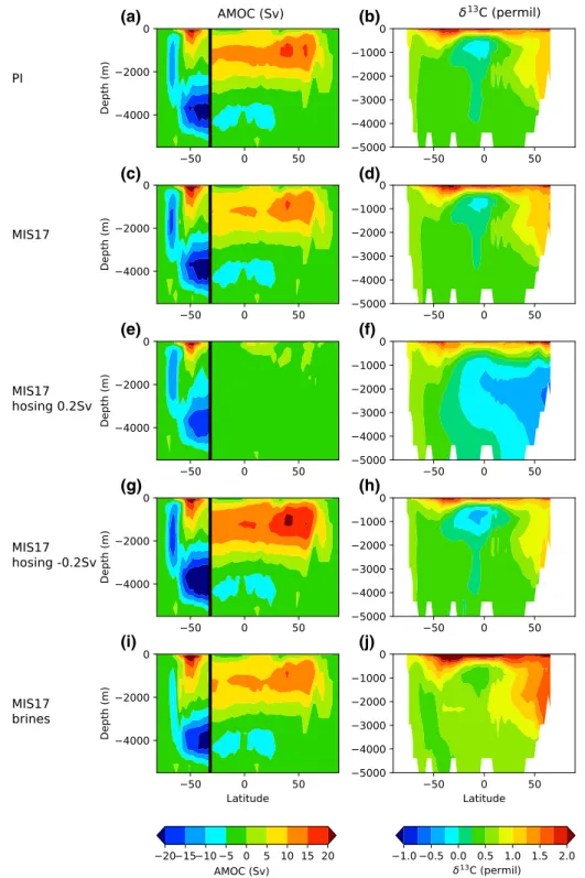
As mentioned before, the change of boundary conditions from the preindustrial to MIS17 (with no other change) yields similar meridional ocean circulations in the Atlantic and Southern Oceans as for the prein-dustrial simulations (Figures 13a and 13c). The maximum of the overturning stream function in the North Atlantic slightly decreases from 17.1 Sv for the preindustrial to 16.6 Sv for MIS17 (Table 4). The max-imum absolute value of the overturning stream function in the Southern Ocean increases from 13.0 Sv dur-ing the PI to 16.6 Sv for MIS17.
The model sensitivity experiments result in a variety of ocean circulations (Figures 13e, 13g, and 13i) con-trasting with the PI and MIS17 ocean circulations (Figures 13a and 13c). Adding a positive fresh waterflux in the North Atlantic (simulation“MIS17 hosing 0.2 Sv”) results in a shutdown of the AMOC (the maximum value of the overturning stream function in the North Atlantic decreases down to 6.5 Sv), while the mini-mum in the Southern Ocean is−15.2 Sv demonstrating a still active cell in this region. Hence this simulation displays a weak North Atlantic circulation but a strong Southern Ocean circulation.
Adding a negative fresh waterflux in the North Atlantic (simulation “MIS17 hosing −0.2 Sv”) leads to an increase of the AMOC with a maximum value of 21.3 Sv in the North Atlantic, but also an active cell in the Southern Ocean with a minimum value of−20.2 Sv. This simulation indicates strong ocean circulation both in the North Atlantic and Southern Oceans.
Finally, the sinking of dense water in the Southern Ocean (simulation“MIS17 brines”) results in a small decrease of the AMOC with a maximum value of 15.9 Sv, but a reduction of the overturning in the Southern Ocean (−10.7 Sv compared to −16.6 Sv in the MIS17 simulation). The overturning in the Southern Ocean is reduced because the salinity at the surface is reduced due to the artificial sinking of dense water by the brine parameterization, which takes a fraction of the salt (frac) rejected by sea ice formation at the surface to put it in the bottom cell. This last example thus displays moderate circulation in the North Atlantic Ocean and reduced circulation in the Southern Ocean.
Figure 12. Mean simulatedδ13C (permil) computed in the“NADW” and “AABW” boxes defined on Figure 9. The mean simulated δ13C in the Pacific between 5° S and 5°N and below 3,000 m is removed.
10.1029/2019PA003776
Paleoceanography and Paleoclimatology
Since the ocean circulation is relatively similar in simulations PI and MIS17, especially in the Atlantic, the δ13C distribution (here shown as a difference with the mean Pacific equatorial signal to compare with data)
is also very much alike (Figures 13b and 13d), except in the Southern Ocean where the increased convection results in more homogenousδ13C values.
Figure 13. Overturning stream function (Sv) (left) andδ13C distribution (permil) (right) in the Atlantic and Southern Ocean (south of 30°S) for the sensitivity experiments. The vertical black line indicates the limit between the Southern Ocean south of 32°S and the Atlantic Ocean north of 32°S. the mean simulatedδ13C in the Pacific between 5°S and 5°N and below 3,000 m is removed.
The AMOC shutdown in simulation“MIS17 hosing 0.2 Sv” leads to much lower δ13C values in the North Atlantic (Figure 13f) because of the absence of convection that previously mixed the13C enriched surface waters (due to biological activity) with the13C depleted deep waters (due to remineralization). Thisδ13C dis-tribution is relatively different from the data shown in Figure 5h, so that such a strong reduction in AMOC can be ruled out.
The negative hosing (simulation“MIS17 hosing −0.2 Sv”) resulting in increased AMOC yields a slight decrease inδ13C values in the North Atlantic especially near the surface (above 100 m) (Figure 13h) where it mixes the deep water mass with lighterδ13C values with the upper water mass with higherδ13C values. In the Southern Ocean, the active circulation maintains relatively high (between 0.5‰ and 1‰) δ13
C values in the oceanic column.
In the last simulation (“MIS17 brines”), the activation of sinking of dense water around Antarctica results in the North Atlantic Ocean in greater penetration of highδ13C values towards the south and the deep ocean compared to“MIS17” experiment (Figure 13j), and higher vertical gradient of δ13C values in the Southern Ocean due to the reduction of convection leading to less mixing of the abyssal water mass with lowδ13C values. Indeed, the parameterization of the sinking of dense water along the continental slopes results in fresher surface water, hence reduced open ocean convection (Bouttes et al., 2010). The reduced mixing results in higherδ13C values in the surface Southern Ocean and hence in higherδ13C values in the atmo-sphere (δ13Catmosphere=−6.33‰) compared to the standard MIS17 simulation (δ13Catmosphere=−6.47‰).
The water that will then penetrate in the deeper ocean will initially have higherδ13C values resulting in lar-gerδ13C values in most regions including the deep South Atlantic.
Hence only the last ocean circulations simulated in“MIS17 brines” leads to higher δ13C distribution in the Atlantic (Figures 14b and 14d) similar to what is indicated by the sediment core data.
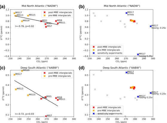
3.7. Consequences on Atmospheric CO2
The data show a good correlation between the atmospheric CO2concentration and the meanδ13C in both
the“NADW” and “AABW” boxes (when the deep equatorial pacific signal is removed) as can be seen on Figures 14a and 14c: The lower CO2 concentrations of pre‐MBE interglacials all go along with higher
mid‐North Atlantic and deep South Atlantic δ13C values (in difference with the equatorial Pacific signal). In the simulations, not only is the change of meanδ13C value in the“NADW” and “AABW” boxes small (red and orange crosses on Figures 14b and 14d), but the change of simulated atmospheric CO2concentration is
also small within interglacial simulations as previously reported (Bouttes et al., 2018). Because small changes of circulation, characterized by small changes ofδ13C, and hence small changes of oceanic carbon storage take place, it results in small atmospheric CO2changes (a few ppm) compared to the larger changes
in the data (~30 ppm).
In the sensitivity experiments, the change of both oceanicδ13C and atmospheric CO2are larger than in the
first set of simulations (blue crosses compared to red and orange on Figures 14b and 14d) but with still a smaller range than the range ofδ13C and atmospheric CO2values from data. Only the simulation with brines
(“MIS17 brines”) results in both higher oceanic δ13C values and lower atmospheric CO2values (9 ppm lower
than the preindustrial run), highlighting the crucial role of abyssal water formation in the Southern Ocean, which is modified in this simulation by the parameterization of sinking of dense water along the continental
Table 4
Maximum and Minimum of the Overturning Circulation Below 500 m
Model simulations
Maximum value in the North Atlantic (Sv)
Minimum value of the Southern Ocean (south of 60°S) (Sv) PI 17.1 −13.0 MIS17 16.6 −16.6 MIS17 hosing 0.2 Sv 6.5 −15.2 MIS17 hosing−0.2 Sv 21.3 −20.2 MIS17 brines 15.9 −10.7
Note. A positive sign indicates a southward circulation, a negative sign a northward circulation.
10.1029/2019PA003776
Paleoceanography and Paleoclimatology
slope around Antarctica. Köhler and Fischer (2006) showed with a box model that a reduced AMOC helped decreasing atmospheric CO2during pre‐MBE interglacials. However, in our simulations, a reduced AMOC,
as has been tested in the simulation with positive fresh waterflux in the North Atlantic (“MIS17 hosing 0.2 Sv”), cannot simultaneously explain the oceanic δ13C and atmospheric CO2changes, and changes in the
Southern Ocean have to be invoked.
4. Conclusions
Theδ13C distribution shown by data is not very different from one interglacial to another at thefirst order (e.g., as compared to LGM changes), with interglacial features common to all interglacials such as high NADWδ13C values. Using meanδ13C for characteristic regions of the Atlantic Ocean, that is, for NADW and AABW, it appears that there is nonetheless a small (~0.2‰) systematic difference before and after the MBE with higherδ13C values before the MBE compared to after.
Despite the small changes in data, the model‐data comparison for the nine interglacials mismatches, with smaller changes in ocean circulation and atmospheric CO2concentration in the simulations as compared
to data. This underlines the potential misrepresentation of ocean circulation changes in the model, possibly due to missing processes or feedbacks, notably related with the low ocean and atmosphere resolution. Sensitivity experiments with modified deep convection in the North Atlantic and Southern Ocean show that δ13C distribution is an order of magnitude larger, which is more in line with the data. Hence, this is
demon-strating that the ocean circulation changes can partly explain some of the changes in atmospheric CO2
con-centration changes. Nevertheless, the atmospheric CO2change simulated in these sensitivity experiments
with larger oceanic circulation changes (~9 ppm) is still lower than shown by the data between post‐ and pre‐MBE interglacials (~30 ppm) and represents only one third of the measured CO2change.
Figure 14. Relationship between (a) data atmospheric CO2concentration (ppm) and data mean oceanicδ13C in the “NADW” box (permil), (b) simulated atmospheric CO2concentration (ppm) and simulated mean oceanicδ13C in the
“NADW” box (permil), (c) data atmospheric CO2concentration (ppm) and data mean oceanicδ13C in the“AABW” box
(permil) and (d) simulated atmospheric CO2concentration (ppm) and simulated mean oceanicδ13C in the“AABW” box
(permil). The data values from (a) and (b) have been plotted in gray on panels (c) and (d). The equatorial Pacific signal has been removed from the meanδ13C values.
Comparison with simulations from other models, especially more complex models, would help towards bet-ter representing the ocean circulation changes. Since the inbet-terglacialδ13C change indicated by data across the MBE is small, the oceanic circulation change across the MBE is probably limited and its impact on car-bon cycle might be too small to explain the entire magnitude of the CO2change between interglacials before
and after the MBE.
Theδ13C changes could also be linked to other changes than ocean circulation, since changes in sea ice, which modifies the atmosphere ocean air exchange, or changes of biological production, could also modify the oceanδ13C values. On land, changes of vegetation could yield atmosphericδ13C modifications, which would then modify oceanicδ13C. Despite all these components being included in the iLOVECLIM model, their changes might not be correctly simulated.
In addition, as only up to a third of the CO2change could be explained in the simulations, it is likely that
other processes are involved. This is further supported by the data as theδ13C gradients are not fundamen-tally different and theδ13C distribution variations across interglacials is not always systematically similar for pre‐ and post‐MBE interglacials. Furthermore, we have removed the mean equatorial Pacific signal linked to the 400‐ka periodicity, and this 400‐ka periodicity could also play a role in the changes across the MBE. For example, changes in the monsoon could impact weathering and in turn the carbon cycle. The burial of organic matter is likely to play an important role (Russon et al., 2010). To test this, it would require to add a sediment model to the climate model to account for such processes. All these mechanisms remain to be tested in climate models during past interglacials to evaluate their possible role in the change of carbon cycle during interglacials of the last 800,000 years.
References
Barth, A. M., Clark, P. U., Bill, N. S., He, F., & Pisias, N. G. (2018). Climate evolution across the mid‐Brunhes transition. Climate of the Past, 14, 2071–2087. https://doi.org/10.5194/cp‐14‐2071‐2018
Bassinot, F. C., Beaufort, L., Vincent, E., Labeyrie, L. D., Rostek, F., Müller, P. J., et al. (1994). Coarse fractionfluctuations in pelagic carbonate sediments from the tropical Indian Ocean: A 1500‐kyr record of carbonate dissolution. Paleoceanography, 9(4), 579–600. https://doi.org/10.1029/94PA00860
Bell, D. B., Jung, S. J. A., Kroon, D., Lourens, L. J., & Hodell, D. A. (2014). Local and regional trends in Plio‐Pleistocene d18O records frombenthic foraminifera. Geochemistry, Geophysics, Geosystems, 15, 3304–3321. https://doi.org/10.1002/2014GC005297
Bereiter, B., Eggleston, S., Schmitt, J., Nehrbass‐Ahles, C., Stocker, T. F., Fischer, H., et al. (2015). Revision of the EPICA Dome C CO2
record from 800 to 600 kyr before present. Geophysical Research Letters, 42, 542–549. https://doi.org/10.1002/2014GL061957 Berger, A. (1978). Long‐term variations of daily insolation and quaternary climatic changes. Journal of the Atmospheric Sciences, 35(12),
2362–2367.
Berger, W. H., Bickert, T., Schmidt, H., & Wefer, G. (1993). Quaternary oxygenisotope record of pelagic foraminifers: Site 806, Ontong JavaPlateau. In L. W. Kroenke & W. H. Berger (Eds.), Proceedings ofthe Ocean Drilling Program, Scientific Results (Vol. 130, pp. 381–395). College Station, TX: Ocean Drilling Program.
Billups, K., Pälike, H., Channell, J., Zachos, J., & Shackleton, N. (2004). Astronomic calibration of the late Oligocene through early Miocene geomagnetic polarity time scale. Earth Planet. Sc. Lett, 224(2004), 33–44.
Bickert, T. (1992). Rekonstruktion der spätquartären Bodenwasserzirkulationim östlichen Südatlantik über stabile Isotope benthischerForaminiferen (Doctoral dissertation). Fachbereich Geowissenschaften, University.
Bickert, T., & Wefer, G. (1996). Late Quaternary deep water circulation in theSouth Atlantic: Reconstruction from carbonate dissolution and benthicstable isotopes. In: G. Wefer, W. H. Berger, G. Siedler, & D. Webb (Eds.), The South Atlantic: Present and Past Circulation (Vol. 103, 599–620). Berlin: Springer‐Verlag.
Bickert, T., Curry, W. B., & Wefer, G. (1997). 16. LatePliocene to Holocene (2.6 Ma) western equatorial Atlantic deep‐watercirculation : inferences from Benthic stable isotopes 1, In N. J. Shackleton, W. B. Curry, C. Richter, & T. J. Bralower, (Eds.), Proceedings of the Ocean Drilling Program(Vol. 154, 239–254). Scientific Results.
Bouttes, N., Paillard, D., & Roche, D. M. (2010). Impact of brine‐induced stratification on the glacial carbon cycle. Climate of the Past, 6, 575–589. https://doi.org/10.5194/cp‐6‐575‐2010
Bouttes, N., Roche, D. M., Mariotti‐Epelbaum, V., & Bopp, L. (2015). Including an ocean carbon cycle model into iLOVECLIM (v1.0). Geosci. Model Dev., 8, 1563–1576. https://doi.org/10.5194/gmd‐8‐1563‐2015
Bouttes, N., Swingedouw, D., Roche, D. M., Sanchez‐Goni, M. F., & Crosta, X. (2018). Response of the carbon cycle in an intermediate complexity model to the different climate configurations of the last nine interglacials. Climate of the Past, 14, 239–253. https://doi.org/ 10.5194/cp‐14‐239‐2018
Brovkin, V., Ganopolski, A., & Svirezhev, Y. (1997). A continuous climate‐vegetation classification for use in climate‐biosphere studies. Ecological Modelling, 101(2–3), 251–261.
Caley, T., Kim, J.‐H., Malaizé, B., Giraudeau, J., Laepple, T., Caillon, N., et al. (2011). High‐latitude obliquity as a dominant forcing in the Agulhas current system. Climate of the Past, 7, 1285–1296. https://doi.org/10.5194/cp‐7‐1285‐2011
Curry, W. B., Duplessy, J. C., Labeyrie, L., & Shackleton, N. J. (1988). Changes in the distribution ofδ13C of deep waterΣCO2between the
last glaciation and the Holocene. Paleoceanography, 3, 317–341.
Chen, J., Farrell, J. W., Murray, D., & Prell, W. L. (1995). Timescale and paleoceanographic implications of a 3.6 m.y. oxygen isotope record from the northeast Indian Ocean (Ocean Drilling Program Site 758). Paleoceanography, 10(1), 21–48. https://doi.org/10.1029/ 94PA02290
10.1029/2019PA003776
Paleoceanography and Paleoclimatology
Acknowledgments
We are thankful to two anonymous reviewers for their comments, which helped improve this manuscript. We also thank Didier Paillard for his help on the 400‐ka signal. The research leading to these results has received funding from the European Union's Horizon 2020 research and innovation program under grant agreement no. 656625, project“CHOCOLATE.” The model outputs are available for download online (doi: 10.5281/ zenodo.3464892).
Cheng, X., Tian, J., & Wang, P. (2004). Data report: Stable isotopes from Site 1143. In W. L. Prell et al. (Eds.), Proceedings of the Ocean Drilling Program, Scientific Results (Vol. 184, pp. 1–8). College Station, TX: Ocean Drilling Program. https://doi.org/10.2973/odp.proc. sr.184.221.2004
Curry, W. B., & Oppo, D. W. (2005). Glacial water mass geometry and the distribution ofδ13C ofΣCO2in the western Atlantic Ocean.
Paleoceanography, 20, PA1017. https://doi.org/10.1029/2004PA001021
deMenocal, P. B., Oppo, D. W., Fairbanks, R. G., & Prell, W. L. (1992). Pleistocene d13C variability of North Atlantic intermediate water. Paleoceanography, 7(2), 229–250. https://doi.org/10.1029/92PA00420
Duplessy, J. C., Shackleton, N. J., Fairbanks, R., Labeyrie, L., Oppo, D., & Kallel, N. (1988). Deep water source variation during the last climatic cycle and their impact on the global deep water circulation. Paleoceanography, 3, 343–360.
Eide, M., Olsen, A., Ninnemann, U. S., & Johannessen, T. (2017). A global ocean climatology of preindustrial and modern oceanδ13C. Global Biogeochem Cycle, 31, 515–534. https://doi.org/10.1002/2016GB005473
Ferretti, P., Crowhurst, S. J., Hall, M. A., & Cacho, I. (2010). North Atlanticmillennial–scale climate variability 910 to 790 ka and the role ofthe equatorialinsolation forcing. Earth and Planetary Science Letters, 293(1–2), 28–41. https://doi.org/10.1016/j.epsl.2010.02.016 Flower, B. P., Oppo, D. W., McManus, J. F., Venz, K. A., Hodell, D. A., & Cullen, J. L. (2000). North Atlantic intermediate to
deep water circulation and chemical stratification during the past 1 Myr. Paleoceanography, 15(4), 388–403. https://doi.org/10.1029/ 1999PA000430
Ganopolski, A., & Calov, R. (2011). The role of orbital forcing, carbon dioxide and regolith in 100 kyr glacial cycles. Climate of the Past, 7, 1415–1425. https://doi.org/10.5194/cp‐7‐1415‐2011
Goosse, H., Brovkin, V., Fichefet, T., Haarsma, R., Huybrechts, P., Jongma, J., et al. (2010). Description of the Earth system model of intermediate complexity LOVECLIM version 1.2. Geosci. Model Dev., 3(2), 603–633. https://doi.org/10.5194/gmd‐3‐603‐2010 Hesse, T., Butzin, M., Bickert, T., & Lohmann, G. (2011). A model‐data comparison of δ13
C in the glacial Atlantic Ocean. Paleoceanography, 26, PA3220. https://doi.org/10.1029/2010PA002085
Hodell, D. A., Channell, J. E. T., Curtis, J. H., Romero, O. E., & Röhl, U. (2008). Onset of "Hudson Strait" Heinrich events in the eastern North Atlantic at the end of the middle Pleistocene transition (~640 ka)? Paleoceanography, 23(4), PA4218. https://doi.org/10.1029/ 2008PA001591
Hodell, D. A., Charles, C. D., Curtis, J. H., Mortyn, P. G., Ninnemann, U. S., & Venz, K. A. (2003). Data Report: Oxygen isotope stratigraphy ofODP Leg 117 sites 1088, 1089, 1090, 1093, and 1094. In R. Gersonde,D. A. Hodell, &P. Blum (Eds.), Proceedings of the Ocean Drilling Program, Scientific Results (Vol. 177, pp. 1–26). College Station, TX: Ocean Drilling Program. https://doi.org/10.2973/odp.proc. sr.177.120.2003
Hoogakker, B. A. A., Rohling, E. J., Palmer, M. R., Tyrrell, T., & Rothwell, R. G. (2006). Underlying causes for long‐term global ocean δ13
C fluctuations over the last 1.20 Myr. Earth and Planetary Science Letters, 248(1‐2) 2006‐08‐15, 15(15), 15–29.
Köhler, P., & Fischer, H. (2006). Simulating low frequency changes in atmospheric CO2during the last 740 000 years. Clim. Pastoralism, 2,
57–78.
Kroopnick, P. (1985). The distribution of13C ofΣCO2in the world oceans. Deep Sea Research I, 32, 57–84.
Lisiecki, L. E. (2010). A simple mixing explanation for late Pleistocene changes in the Pacific‐South Atlantic benthic δ13
C gradient. Climate of the Past, 6, 305–314. https://doi.org/10.5194/cp‐6‐305‐2010
Lisiecki, L. E., & Raymo, M. E. (2005). A Pliocene‐Pleistocene stack of 57 globally distributed benthic δ18
O records. Paleoceanography, 20(1), PA1003. https://doi.org/10.1029/2004PA001071
Lüthi, D., Le Floch, M., Bereiter, B., Blunier, T., Barnola, J.‐M., Siegenthaler, U., et al. (2008). High‐resolution carbon dioxide concentration record 650,000‐800,000 years before present. Nature, 453(7193), 379–382. https://doi.org/10.1038/nature06949
Malaizé, B., Jullien, E., Tisserand, A., Skonieczny, C., Grousset, E., Eynaud, F., & Schneider, R. (2012). The impact of African aridity on the isotopic signature of Atlantic deep waters across the Middle Pleistocene Transition. Quaternary Research, 77(1), 182–191. https://doi.org/ 10.1016/j.yqres.2011.09.010
Marchal, O., & Curry, W. B. (2008). On the abyssal circulation in the glacial Atlantic. Journal of Physical Oceanography, 38, 2014–20,370. Martínez‐Méndez, G., Hebbeln, D., Mohtadi, M., Lamy, F., De Pol‐Holz, R., Reyes‐Macaya, D., & Freudenthal, T. (2013). Changes in
theadvection of Antarctic Intermediate Water to the northern Chileancoast during the last 970 kyr. Paleoceanography, 28(4), 607–618. https://doi.org/10.1002/palo.20047
McManus, J. F., Oppo, D. W., & Cullen, J. L. (1999). A 0.5-million-year record of millennial-scale climate variability in the North Atlantic. Science, 283, 971–975.
Menviel, L., Mouchet, A., Meissner, K. J., Joos, F., & England, M. H. (2015). Impact of oceanic circulation changes on atmosphericδ13CO2.
Global Biogeochem Cycle, 29, 1944–1961. https://doi.org/10.1002/2015GB005207
Mix, A. C., Pisias, N. G., Zahn, R., Rugh, W., Lopez, C., & Nelson, K. (1991). Carbon 13 in Pacific Deep and Intermediate Waters, 0-370 ka: Implications for Ocean Circulation and Pleistocene CO2. Paleoceanography, 6(2), 205–226. https://doi.org/10.1029/90PA02303 Mix, A. C., Pisias, N. G., Rugh, W., Wilson, J., Morey, A., & Hagelberg, T. (1995). Benthic foraminifera stable isotope record form site 849,
0‐5 Ma: Local and global climate changes. In N. G. Pisias et al. (Eds.), Proceedings of the Ocean Drilling Program, Scientific Results (Vol. 138, pp. 371–412). Texas, USA: College Station.
Oliver, K. I. C., Hoogakker, B. A. A., Crowhurst, S., Henderson, G. M., Rickaby, R. E. M., Edwards, N. R., & Elderfield, H. (2010). A synthesis of marine sediment coreδ13C data over the last 150 000 years. Climate of the Past, 6, 645–673. https://doi.org/10.5194/ cp‐6‐645‐2010
Oppo, D. W., Fairbanks, R. G., Gordon, A. L., & Shackleton, N. J. (1990). Late Pleistocene Southern Ocean d13C variability. Paleoceanography, 5(1), 43–54. https://doi.org/10.1029/PA005i001p00043
Oppo, D. W., McManus, J. F., & Cullen, J. L. (1998). Abrupt climate events 500,000–340,000 years ago: Evidence fromsubpolar North Atlantic sediments. Science, 279, 1335–1338.
Paillard, D. (2017). The Plio‐Pleistocene climatic evolution as a consequence of orbital forcing on the carbon cycle. Climate of the Past, 13, 1259–1267. https://doi.org/10.5194/cp‐13‐1259‐2017
Paillard, D., & Donnadieu, Y. (2014). A 100 Myr history of the carbon cycle based on the 400 kyr cycle in marineδ13C benthic records. Paleoceanography, 29, 1249–1255. https://doi.org/10.1002/2014PA002693
Paillard, D., Labeyrie, L., & Yiou, P. (1996). Macintosh program performs time‐series analyses. Eos Trans. AGU, 77(39), 379.
Pälike, H., Norris, R. D., Herrle, J. O., Wilson, P. A., Coxall, H. K., Lear, C. H., et al. (2006). The heartbeat of the Oligocene climate system. Science, 314(5807), 1894–1898. https://doi.org/10.1126/science.1133822
Past Interglacials Working Group of PAGES (2016). Interglacials of the last 800,000 years. Reviews of Geophysics, 54, 162–219. https://doi. org/10.1002/2015RG000482
Poirier, R. K., & Billups, K. (2014). The intensification of northern component deepwater formation during the mid‐Pleistocene climate transition. Paleoceanography, 29, 1046–1061. https://doi.org/10.1002/2014PA002661
Raymo, M. E., Ruddiman, W. F., Backman, J., Clement, B. M., & Martinson, D. G. (1989). Late Pliocene variation in northern hemisphere icesheets and North Atlantic deep water circulation. Paleoceanography, 4(4), 413–446. https://doi.org/10.1029/PA004i004p00413 Raymo, M. E., Oppo, D. W., & Curry, W. (1997). The mid-Pleistocene transition: A deep sea carbon isotopic perspective, Paleoceanography,
12, 546–559
Raymo, M. E., Oppo, D. W., Flower, B. P., Hodell, D. A., McManus, J. F., Venz, K. A., et al. (2004). Stability ofNorth Atlantic water masses in face of pronounced climate variability during the Pleistocene. Paleoceanography, 19, PA2008. https://doi.org/10.1029/2003PA000921 Roche, D. M., Wiersma, A. P., & Renssen, H. (2010). A systematic study of the impact of freshwater pulses with respect to different
geo-graphical locations. Climate Dynamics, 34(7‐8), 997–1013. https://doi.org/10.1007/s00382‐009‐0578‐8
Ruddiman, W. F., Raymo, M. E., Martinson, D. G., Clement, B. M., & Backman, J. (1989). Pleistocene evolution: Northern hemisphere ice sheets andNorth Atlantic Ocean. Paleoceanography, 4(4), 353–412. https://doi.org/10.1029/PA004i004p00353
Russon, T., Paillard, D., & Elliot, M. (2010). Potential origins of 400–500 kyr periodicities in the ocean carbon cycle: A box model approach. Global Biogeochemical Cycles, 24, GB2013. https://doi.org/10.1029/2009GB003586
Sarnthein, M., & Tiedemann, R. (1989). Towarda high-resolution stable isotope stratigraphy of the last 3.4 million years: Sites 658 and 659 off Northwest Africa. In W. F. Ruddiman et al. (Eds.), Initial Reports of the Deep Sea Drilling Project (Vol. 108, pp. 167–185). Washington, DC: U.S. Government Printing Office.
Schlitzer, R. (2017). Ocean Data View. http://odv.awi.de
Schmittner, A., Gruber, N., Mix, A. C., Key, R. M., Tagliabue, A., & Westberry, T. K. (2013). Biology and air–sea gas exchange controls on the distribution of carbon isotope ratios (δ13C) in the ocean. Biogeosciences, 10, 5793–5816. https://doi.org/10.5194/bg-10-5793-2013
Sexton, P., Norris, R. D., Wilson, P. A., Pälike, H., Westerhold, T., Röhl, U., et al. (2011). Eocene global warming events driven by ventilation of oceanic dissolved organic carbon. Nature, 471(7338), 349–352. https://doi.org/10.1038/nature09826
Shackleton, N. J., & Hall, M. A. (1984). Oxygen and carbon isotope stratigraphy of deep‐sea drilling project HOLE‐552A: Plio‐Pleistocene glacial history. Initial reports of the deep sea drilling project (Vol. 81, pp. 599–609). Washington, DC: U.S. Government Printing Office. Shackleton, N. J., & Hall, M. A. (1989). Stable isotope history of the Pleistocene at ODP Site 677. In K. Becker, H. Sakai, et al. (Eds.),
Proceedings of the Ocean Drilling Program, Scientific Results, (Vol. 111, pp. 295–316). College Station, TX: (Ocean Drilling Programm). https://doi.org/10.2973/odp.proc.sr.111.150.1989
Shackleton, N. J., & Opdyke, N. D. (1973). Oxygen isotope and palaeomagnetic stratigraphy of equatorial Pacific core V28‐238: Oxygen isotope temperatures and ice volumes on a 105year and 106year scale. Quaternary Research, 3, 39–55. https://doi.org/10.1016/0033‐5894 (73)90052‐5
Tian, J., Ma, X., Zhou, J., Jiang, X., Lyle, M., Shackford, J., & Wilkens, R. (2018). Paleoceanography of the east equatorial Pacific over the past 16 Myr and Pacific–Atlantic comparison: High resolution benthic foraminiferal δ18
O andδ13C records at IODP Site U1337. Earth and Planetary Science Letters, 499, 185–196.
Venz, K. A., & Hodell, D. A. (2002). New evidence for changesin Plio‐Pleistocene deep water circulation from Southern Ocean ODPLeg 177 Site 1090. Palaeogeography,palaeoclimatology, palaeoecology, 182(3‐4), 197–220
Venz, K., Hodell, D. A., Stanton, C., & Warnke, D. A. (1999). A 1.0 Myr record of Glacial North Atlantic Intermediat eWater variability from ODP site 982 in the northeast Atlantic. Paleoceanography, 14, 42–52.
Voelker, A. H. L., Rodrigues, T., Billups, K., Oppo, D. W., McManus, J. F., Stein, R., et al. (2010). Variations inmid-latitudeNorth Atlantic surface water properties during the mid-Brunhes (MIS9-14) and their implications for the thermohaline circulation. Climate of the Past, 6(4), 531–552. https://doi.org/10.5194/cp‐6‐531‐2010
Wang, P., Tian, J., Cheng, X., Liu, C., & Xu, J. (2004). Major Pleistocene stages in a carbon perspective: The South China Sea record and its global comparison. Paleoceanography, 19, PA4005. https://doi.org/10.1029/2003PA000991
Wang, P., Tian, J., & Lourens, L. (2010). Obscuring of long eccentricity cyclicity in Pleistocene oceanic carbon isotope records. Earth and Planetary Science Letters, 290, 319–330.
Wright, A. K., & Flower, B. P. (2002). Surface and deep ocean circulation in the subpolar North Atlantic during the mid‐Pleistocene revolution. Paleoceanography, 17(4), 1068. https://doi.org/10.1029/2002PA000782
Yin, Q. (2013). Insolation‐induced mid‐Brunhes transition in Southern Ocean ventilation and deep‐ocean temperature. Nature, 494(7436), 222–225. https://doi.org/10.1038/nature11790
Yin, Q. Z., & Berger, A. (2010). Insolation and CO2contribution to the interglacial climate before and after the mid‐Brunhes event. Nature
Geoscience, 3, 243–246. https://doi.org/10.1038/ngeo771
Yin, Q. Z., & Berger, A. (2012). Individual contribution of insolation and CO2to the interglacial climates of the past 800,000 years. Climate
Dynamics, 38(3–4), 709–724.