An equilibrium approach for Gamma Discounting

An equilibrium approach for Gamma Discounting

Elyès Jouini

and Clotilde Napp

February 13, 2009

Abstract

We address the problem of a social planner who, as in Weitzman (2001), gath-ers data on discount rates and wants to infer the socially e¢ cient consumption discount rate. We propose an equilibrium approach and we analyse the expres-sion and the properties of the resulting equilibrium discount rate. We provide equilibrium foundations for Gamma discounting at the collective level even though individual agents are classical exponential discounters. We analyse the impact of shifts in the distributions of individual discount rates on the shape of the yield curve. Finally, we apply our approach to Weitzman (2001)’s data to propose discount rates for public sector Cost-Bene…t Analysis, in particular for the long term.

Key-words: consumption discount rate; equilibrium discount rate; experts dis-count rate; hyperbolic disdis-counting; cost-bene…t analysis; gamma disdis-counting; divergence of opinion;

1

Introduction

The appropriate social discount rate to apply in public sector cost-bene…t analysis is a contentious issue. This is especially true for long term projects, for which …nancial markets cannot provide any guideline. As Weitzman (2001, p.261) states “There

The …nancial support of the GIP-ANR ("Croyances" project) and of the Risk Foundation (Groupama chair) is gratefully acknowledged.

y_{Université Paris-Dauphine, Ceremade, F-75016 Paris, France, jouini@ceremade.dauphine.fr,}

phone: + 33 1 44 05 42 26

z_{CNRS, UMR7088, F-75016 Paris, France}

x_{Université Paris-Dauphine, DRM, F-75016 Paris, France, clotilde.napp@dauphine.fr, phone: +}

does not now exist, nor has ever existed, anything remotely resembling a consensus, even -or, perhaps one should say especially- among the ‘experts’on this subject”.

In this paper we address the problem of a social planner, who gathers data on discount rates and wants to infer the socially e¢ cient discount rate. More precisely, as in Weitzman (2001), the social planner has conducted a survey about the discount rate to apply for costs or bene…ts occurring at a given date t; each participant to the survey has proposed a discount rate and the problem of the social planner is to aggregate these proposed discount rates into a socially e¢ cient discount rate.

As underlined by e.g. Nordhaus (2007) or Weitzman (2007), there is an impor-tant distinction between the utility social discount rate and the consumption social discount rate. The former refers to a pure time preference rate that discounts util-ity. It re‡ects the level of impatience or, for long time horizon projects, the relative weights of di¤erent people or generations. The latter is the rate used to discount future consumption; it is determined by the time preference rate, but also by the anticipations about the future of the economy. The (extended) Ramsey equation1

illustrates the distinction and the relation between the utility discount rate and the consumption discount rate. Letting R denote the consumption discount rate, and the utility discount rate, Ramsey formula gives the relation R = + 1₂ (1 + ) 2_,

where is the growth rate of the economy and is the elasticity of marginal util-ity. Apart in the speci…c settings of a stationary economy ( = = 0) or a risk neutral investor ( = 0) or when the wealth and precautionary savings e¤ect cancel out ( = 1₂(1 + ) 2_{), the two rates di¤er. In this paper, the rates proposed in the}

survey, as well as the socially e¢ cient discount rate to be inferred, are consumption discount rates, since they are to be applied to cost-bene…t analysis. This is also the case in Weitzman (2001); indeed, as Weitzman makes it clear in his question-naire : “What I am here after is the relevant interest rate for discounting real-dollar changes in future goods and services –as opposed to the rate of pure time preference on utility”2_.

Weitzman (1998, 2001) deal with this problem by adopting a certainty equivalent approach. In this certainty equivalent approach, the social discount factor is taken to be the (arithmetic) average of the discount factors associated to the individual dis-count rates. Weitzman (1998) derives properties of the certainty equivalent disdis-count rate and in particular, its convergence towards the lowest individual discount rate,

1_{The original Ramsey equation (Ramsey, 1928) was derived in a deterministic setting ( = 0)}

and is given by R = + : The extended Ramsey equation corresponds to a direct generalization in a stochastic setting. For the sake of completeness, we rederive it in the Appendix.

2_{Moreover, the fact that the given rates are on average equal to 4% con…rms that they are}

whatever the distribution of individual discount rates. Weitzman (2001) applies this approach to a speci…c example. Starting from the results of a survey based on the opinions of 2,160 economists about the consumption discount rate, he estimates its distribution and derives an explicit expression for the certainty equivalent discount rate in this case (Gamma discounting). Gollier (2004) underlines that the approach of Weitzman (1998, 2001) amounts to ranking the projects according to their expected net present value. By adopting the criterion that projects should be ranked accord-ing to their expected future value, Gollier (2004) reaches opposite conclusions and concludes that “both criteria are arbitrary as they do not rely on realistic preferences of human beings towards risk and time” suggesting that an equilibrium analysis is maybe the cost to be paid to make policy recommendations that have an economic sense.

We propose an approach that relies on an equilibrium analysis. We consider that each proposed rate corresponds to a speci…c calibration of Ramsey formula and re‡ects then the pure time preference rate _i (or as previously underlined, the con-ception of intergenerational equity) and the beliefs ( i; i) about the future growth

of the economy of the individual under consideration. The divergence in the pro-posed individual discount rates Ri _{stems then from divergence in individual tastes}

and beliefs. We consider that the participants to the survey are representative in the sense that each of them represents the tastes and beliefs of the same portion of the population. It is then natural to adopt as the socially e¢ cient discount rate the equilibrium discount rate in the economy made of agents with the heterogeneous beliefs and tastes of the participants to the survey. For example, if the panel is made of three participants, the …rst one proposing the discount rate R1_{; the}

sec-ond R2 _{and the third R}3 _{corresponding respectively to characteristics (}

1; 1; 1),

( ₂; ₂; 2) and ( 3; 3; 3) ; then we take as the socially e¢ cient discount rate the

equilibrium discount rate in an economy made of one third of agents with character-istics ( 1; 1; 1), one third of agents with characteristics ( 2; 2; 2) and one third

of agents with characteristics ( 3; 3; 3) : This means that we have transformed the

problem of aggregating data on heterogeneous discount rates into the problem of aggregating data on heterogeneous beliefs and tastes.

We can then apply the techniques3 of Jouini et al. (2008) in order to obtain the expression of the socially e¢ cient discount rate. If we let At denote the price at date

0of a zero coupon bond maturing at date t; the average discount rate between date 0 and date t is given by Rt 1_tln At and the marginal discount rate is given by

rt A

0 t

At. We obtain that both rates are weighted averages of the individual discount

3_{Jouini et al. (2008) deals with the determination of the equilibrium discount rate in an economy}

rates. They are both decreasing with time and converging to the lowest individual expert discount rate.

In the present paper we consider logarithmic utility functions. There are essen-tially two reasons for such a restriction. The …rst reason is analytical tractability. Indeed, as underlined by Rubinstein (1975), “log utility functions are singular in their capacity to cope with heterogeneous beliefs while not imposing unreasonable restrictions on tastes”. This choice enables us to obtain simple formula, while con-sidering reasonable levels of risk aversion4. The second reason is the central role of logarithmic utility functions. Jouini et al. (2008) shows that the log-utility setting is central in the analysis of beliefs heterogeneity: some biases are induced when we deal with power utility function c₁1 with _{6= 1; these biases being in opposite directions} depending on the position of with respect to 1. This is then an additional argument in favor of the log-utility setting. Note …nally that the choice of = 1 is also made in the Stern Review.

We compare our expression for the socially e¢ cient discount rate with other pos-sible functions of the individual discount rates previously considered in the literature. In particular, our formula are di¤erent from Weitzman (1998). The equilibrium dis-count rate coincides with Weitzman (1998, 2001) certainty equivalent disdis-count rate only when all individuals have the same pure time preference rate. In a more general setting, the discount rates of the more impatient individuals are granted a higher weight. A possible interpretation is as follows. When considering its intertemporal rate of substitution, the group must weigh more the agents with a higher shadow price of the intertemporal budget constraint, i.e. the more impatient members of the group. The overweighting of impatient individuals’discount rates implies that when tastes and beliefs are independent, the equilibrium discount rate is higher than the certainty equivalent discount rate for all horizons.

We determine the explicit expression of the socially e¢ cient discount rate for speci…c distributions of the individuals’ discount rates. We consider Gaussian as well as Gamma distributions. We calibrate the model with a Gamma distribution on Weitzman (2001)’s data. Our results suggest using the following approximation of within-period marginal discount rates for long term public projects: Immediate Future about 5 per cent; Near Future about 4 percent; Medium Future about 3 percent; Distant Future about 1.5 per cent and Far-Distant Future about 0 per cent. Except for the Far-Distant Future, these rates are slightly higher than those obtained by Weitzman (2001) .

Finally, we determine which concepts of stochastic dominance on the distribu-tions of individual discount rates lead to a clear impact on the equilibrium discount

rate. We analyze the impact of standard shifts, like …rst or second stochastic dom-inance shifts as well as monotone likelihood ratio domdom-inance shifts. The impact of these shifts are di¤erent depending on which discount rate (average or marginal) we consider. Roughly speaking, more pessimism, more patience, more doubt as well as more heterogeneity in individual discount rates reduce the equilibrium discount rate. Note that our approach also permits to aggregate utility discount rates5 _(pure

time discount rates). It su¢ ces to consider the speci…c case where there is no beliefs heterogeneity. We obtain that the equilibrium utility discount rate is a weighted av-erage of the individual ones. Our formulas are then analogous to those of Lengwiler (2005). They coincide with those of Nocetti et al. (2008) and Gollier and Zeckhauser (2005) only for speci…c choices of Pareto weights. They di¤er from those in Rein-schmidt (2002), in the same way as our formulas for the consumption discount rate di¤er from those in Weitzman (1998). We emphasize that, while these papers aim at aggregating individual utility discount rates, the aim of the present paper is to aggregate individual consumption discount rates and to do it through an equilibrium approach.

All proofs are in the Appendix.

2

Equilibrium discount rate

Let us consider n individuals, who propose di¤erent discount rates (Ri_{) for}

cost-bene…t analysis of public projects as in Weitzman (2001):

We assume that the discount rate proposed by individual i for costs or bene…ts occurring at date t corresponds to a speci…c parametrization of the extended Ramsey equation (see the Appendix), i.e., that the consumption discount rate Ri proposed by individual i is given by

Ri = _i+ _i 2_i where _i > 0; _i and 2

i are respectively the pure time preference rate, the mean

and the variance (by unit of time) of the distribution of the growth rate of aggregate consumption that the individual uses in order to calibrate the model. The divergence on the discount rates (Ri_{)results then from divergence on these parameters.}

Assuming that agents di¤er in their expectation about the growth rate is fairly natural. Indeed, the expected growth rate re‡ects the opinion about the future. It

5_{The problem of aggregating individual utility discount rates has been studied by, among others,}

Reinschmidt (2002) through a certainty equivalent approach, Nocetti et al. (2008) through a Ben-thamite approach, Gollier-Zeckhauser (2005) through a Pareto optimality approach and Lengwiler (2005) through an equilibrium approach.

su¢ ces to look at experts forecasts to realise that there is no consensus about the future of the economy. Indeed, forecasting for the coming year is already a di¢ cult task. It is natural that forecasts for the next century/millennium are subject to potentially enormous divergence. It is doubtful that agents or economists currently have a complete understanding of the determinants of long term economic evolutions. It is also natural to assume that individuals di¤er in their pure time preference rate since it may re‡ect their point of view about intergenerational equity as well as one’s level of impatience. The important debate among economists (and also among philosophers) on the notion of intergenerational equity is an illustration of this possible divergence. Some will argue that intergenerational choices should be treated as intertemporal individual choices leading to weigh more present welfare. Others will argue that fundamental ethics require intergenerational neutrality and that the only ethical basis for placing less value on the welfare of future generations is the uncertainty about whether or not the world will exist and whether or not these generations will be present.

The problem now is to determine how to aggregate these discount rates into a consensus discount rate. We consider that the panel’s tastes and beliefs re‡ect those of the population. We shall then consider a complete markets economy with heterogeneous agents endowed with the beliefs and tastes of the agents in the panel and we shall adopt the equilibrium discount rate in this economy as our consensus discount rate.

To summarise, we have N groups of agents,

wi relative size of group i,

i pure time preference rate of the agents in group i,

t the time at which a cost or bene…t is incurred, relative to the present time, a date 0 total consumption e0 normalized to 1

ln_{N (( i} 1₂ 2

i)t; 2it) group i’s anticipated distribution6 of aggregate

con-sumption et at date t,

log utility functions,

6_{This is the case for instance if aggregate consumption is a geometric Brownian motion with}

Ri

i + i 2i, the individual discount rate for agents in group i, i.e. the

equilibrium discount rate that would prevail if the economy was made of group iagents only.

The weights wi model then the distribution of agents characteristics in the

econ-omy, which also corresponds, by construction, to the distribution of the survey par-ticipants characteristics.

2.1

Expression of the equilibrium discount rate and

proper-ties

We let Mi denote the density of agenti’s belief with respect to a given reference probability P . An Arrow-Debreu equilibrium is de…ned by a state price q_t and op-timal consumption plans y i

i=1;:::;N such that each group maximizes its aggregate

utility R₀1exp( _it)E [Mi

tlog yit] dt under its budget constraint

R₁ 0 E P _[q tyti] dt wi R1 0 E P_[q

tet] dt and markets clear i.e.,

PN i=1y

i

= e.

We denote by At the equilibrium discount factor for horizon t, i.e. the price at

date 0 of $1 at date t: We denote by Rt 1_tln Atthe discount rate for horizon t, i.e.

the rate which if applied constantly for all intervening years would yield the discount factor At: We denote by rt

A0 t

At the marginal discount rate for horizon t, i.e. the

rate of change of the discount factor. We have Rt= 1_t

Rt

0 rsds: Marginal and average

discount rates coincide when the discount rate is constant. In particular, for all i, the individual marginal discount rate ri _{coincides with the individual discount rate}

Ri_{: However, the distinction between the two notions of discount rates can become}

important when the discount rate is time dependent (Groom et al., 2005).

Applying the techniques of Jouini et al. (2008, Proposition 5.1), we easily get that the average discount rate Rt is given by

Rt 1 t ln N X i=1 w_{i i} PN j=1wj j exp Rit; (1)

that it decreases with t and that it converges to the lowest proposed rate R₁ = infiRi:For the sake of completeness (and because the settings are slightly di¤erent),

we provide the proof of Equation (1) at the beginning of the Appendix.

Proposition 1 1. The equilibrium marginal discount rate is given by rt N X i=1 w_{i i}exp ( ri_t) PN j=1wj jexp ( rjt) ri: (2)

2. In the case of homogeneous beliefs ( _i = ; i = ), the equilibrium marginal

discount rate is given by rt N X i=1 w_{i i}exp ( _it) PN j=1wj jexp jt i+ 2_{: (3)}

3. The discount rate rt decrease with t; and the asymptotic equilibrium discount

rate is given by the lowest individual discount rate, i.e. r₁= infiri = R1:

As in the certainty equivalent approach of Weitzman (1998), the consensus dis-count factors obtained through our equilibrium approach are averages of the in-dividual discount factors. However, except in the case of homogeneous pure time preference rates, i.e. i = for all i, our expressions for the rates are di¤erent from

those of Weitzman (1998). There is a bias towards the more impatient agents in the consensus equilibrium discount rates. A possible interpretation is as follows. When considering its intertemporal rate of substitution, the group must weigh more the agents with a higher shadow price of the intertemporal budget constraint, i.e. the more impatient members of the group.

As far as asymptotic properties are concerned, we obtain that the relevant rate in the long run is given by the lowest individual discount rate. This rate corresponds to the discount rate of the most patient agent (lowest i) when there is no beliefs

heterogeneity, or to the most pessimistic agent (lowest i) when there is no pure time

preference rate heterogeneity and all the agents have the same volatility parameter or to the least con…dent agent (highest 2

i) when there is no pure time preference

rate heterogeneity and all the agents have the same drift parameter. Moreover, the equilibrium approach leads to decreasing discount rates, not only utility discount rates, but also consumption discount rates. As in the certainty approach of Weitzman (1998), this leads to use lower discount rates for long term projects in a cost-bene…t analysis.

In the case of homogeneous beliefs, Equation (3) involves the covariance between

i and exp it as in Lengwiler (2005). Equation (3) also gives us the expression

for the consensus utility discount rate PN_i=1 wi iexp( it)

PN

j=1wj jexp( jt) i. Although of the

optimality of Gollier and Zeckhauser (2005) or the Benthamite approach of Nocetti et al. (2008). Indeed, our weights in the weighted averages of the i are given by

the quantities w_{i i}exp _it whereas they are given by iexp it in Gollier and

Zeckhauser (2005) or Nocetti et al. (2008), where the ( i)are Pareto weights chosen

by the social planner. Notice that this means that our equilibrium approach and the Pareto/Benthamite approach would lead to the same social utility discount rate only if the Pareto weights were proportional to w_{i i}. Conversely, if the ( i)and the wi are

independent from the is, then more impatient agents are more heavily weighted.

2.2

Comparison with other formula for the socially e¢ cient

discount rate

The following proposition clari…es the relation between our socially e¢ cient discount rate and the di¤erent expressions that have been provided in the literature.

Proposition 2 1. The equilibrium discount rate is lower than the pure time pref-erence weighted arithmetic average of the individual discount rates, i.e.

Rt N X i=1 w_{i i} PN j=1wj j Ri and rt N X i=1 w_{i i} PN j=1wj j ri: (4)

2. If the tastes and beliefs characteristics _i and bi i 2i are independent

or if they are comonotonic, i.e. individuals with higher tastes characteristics

i have higher beliefs characteristics bi, then the equilibrium discount rate is

higher than an average of the individual discount rates, i.e. Rt 1 t ln N X i=1 wiexp Rit: (5)

3. If the tastes and beliefs characteristics _i and bi i 2i are independent,

then the equilibrium marginal discount rate is higher than an average of the individual marginal discount rates, i.e.

rt N X i=1 wiexp rit PN j=1wjexp rjt ri: (6)

Equation (4) means that, as expected, the discount rate to use is lower than the simple arithmetic average (with the same weights) of the individual discount rates. Moreover, Equations (5) and (6) imply that, when tastes and beliefs characteristics are independent, our discount rates are higher than those of Weitzman (2001). This is intuitive since our weights are given by the pure time preference rates i hence

higher weights are granted to higher individual discount rates.

3

Speci…c Distributions and Dominance

Proper-ties

Let us now determine the equilibrium discount rate for speci…c distributions of the individual discount rates (Ri_{) : Equation (1) as well as Proposition 1 provide the}

expression of the discount rates R and r as a function of the individual discount rates (Ri_{) or (r}i_{) :}

3.1

Gaussian and Gamma distributions

We whall consider continuous sets of individuals. It is easy to show that the expres-sion of the discount rates remains the same in the setting with a continuum of agents. The problem is that according to Equations (1) and (2), we need to make extra as-sumptions on the joint distribution of ( i; Ri) in order to determine the discount

rates R and r.

Consider …rst the case with homogeneous pure time preference rates i = ;and

with a normal distribution N (m; v2) on the beliefs parameters bi = i 2i: The

discount rates (Ri₎

then follow a normal distribution N ( + m; v2_{) and we easily}

obtain that Rt= + m v

2

2 t: Reinschmidt (2002) obtains a similar formula for the

consensus utility discount rate when the individual utility discount rates follow a normal distribution.

Suppose now that utility discount rates and beliefs are independently7_{and gamma}

distributed. We obtain the following result.

Proposition 3 If pure time preference rates i and beliefs bi = i 2i are

indepen-dently distributed8 _with

i ( 1; 1) and bi ( 2; 2); then

7_{We focus on the case of independent distributions as a central case; explicit formulas may also}

be derived in the case of a given correlation between pure time preference rates and beliefs.

8_{Recall that the density function of a gamma distribution ( ; ) is given by} ( )x

1_{exp( x):}

Its mean m and its variance v2 _{are respectively given by m = and}

1. Rt = 1_t+1ln 1 1+t 2 t ln 2 2+t and rt = 1+1 1+t + 2 2+t = m2 1+v21 m1+tv21 + m22 m2+tv2 where

(m1; v12) and (m2; v22) respectively denote the mean and variance of ( i) and

(bi) : 2. If ₁ = ₂ then Ri _{( ; ) with =} 1+ 2; Rt = RWt + 1tln 1 + t _and rt = m 2_+v2 m+tv2 = r W t + +t1 where r W

t and RWt respectively denote the marginal

discount rate and the discount rate obtained through the certainty equivalent approach of Weitzman and where (m; v) denote the mean and variance of (Ri_{) :}

A decrease in the mean m2 or an increase in the variance v22 of the individual

beliefs (bi) decreases the marginal discount rate rt (hence the discount rate Rt).

The same result occurs with a decrease in the mean m1 of the individual pure time

preference rates ( _i). An increase in the variance v2

1 of the individual pure time

preference rates ( i) decreases the marginal discount rate rt for t large enough.

When beliefs and tastes are independent and follow gamma distributions with the same parameter ; the distribution of the individual discount rates Ri _{or r}i _{is a su¢}

-cient statistics for the equilibrium discount rate. As in Weitzman (2001), individual discount rates then follow a Gamma distribution. As shown in the previous section, our equilibrium discount rates are higher than Weitzman (2001)’s discount rates but converge to the same value. A decrease in the mean m of the individual discount rates (Ri_{)decreases the marginal discount rate and an increase in the variance v}2 _of

the individual discount rates (Ri_{) decreases the marginal discount rate r}

t for t large

enough.

3.2

Calibration on Weitzman (2001)’s data

We now calibrate this model with two independent gamma distributions i ( 1; 1)

and bi ( 2; 2) on Weitzman (2001)’s data. We impose that m1 + m2 = m

and v2

1 + v22 = v2 where m and v2 respectively denote the mean and the variance

of the individual discount rates computed on Weitzman(2001)’s sample. We fur-ther impose that m1

v1 =

m2

v2 (same ratio between mean and standard deviation for

both distributions), which leads to 1 = 2 and 1

2 =

m2

m1 ; for some positive

: Note that for = 1, we get ( 1; 1; 2; 2) = m2 2v2; m v2; m2 2v2; m v2 ; which

corre-sponds to the calibration in Weitzman (2001). We have then a family of stastis-tical models that contains Weitzman (2001)’s statisstastis-tical model and we maximize the log-likelihood with respect to the parameter to choose the best calibration. We obtain = 0:4116 hence ( 1; 1; 2; 2) = (1:043; 89:454; 1:043; 36:819) and

(m1; v12; m2; v22) = (1:16 10 2; 1:30 10 4; 2:83 10 2; 7:69 10 4). To summarise,

the best calibration corresponds to a gamma distribution on the individual pure time preference rates with an average time preference rate among experts equal to 1:16% and a median equal to 0:67% and a gamma distribution on the individual beliefs with an average belief parameter (about the growth of the economy) equal to 2:83% and a median equal to 2%: More precisely, the belief parameter b = 2 _{can be}

interpreted as a risk adjusted growth rate. The values we obtain are then reasonable values for both an average pure time preference rate and an average risk-adjusted growth rate. Stern report considers values for the pure time preference rate (utility discount rate) between 0.1 and 1.5 and values for the growth rate ranging from 0 per cent to 6 per cent. Arrow (1995) states that the pure time preference rate should be about 1% and surveying the evidence, the HM Treasury’s Green Book (2003) suggests a long run growth rate of 2.1 per cent.

Figure 1 represents the log-likelihood as a function of : Figure 2 represents the distribution of the individual discount rates for the parameter that maximizes the log-likelihood ( = 0:4116) as well as the empirical distribution and Weitzman (2001)’s distribution. Figure 3 represents the corresponding marginal discount rate curve and compares it to the discount rate curve of Weitzman (2001). Table 1 presents the corresponding recommended sliding-scale discount rates: Immediate Future about 5 per cent; Near Future about 4 percent; Medium Future about 3 percent; Distant Future about 1.5 per cent and Far-Distant Future about 0 per cent.

3.3

Dominance properties

In the speci…c setting of Gamma distributions considered in Proposition 3, we have seen the impact of an increase in the mean and in the variance of the distribution of individual discount rates on the socially e¢ cient discount rates. The impact was the same for the average and for the marginal discount rates. We now analyze in a more general setting which shifts on the distribution of individual discount rates have a clear impact on the socially e¢ cient discount rates. We consider First and Second Stochastic Dominance shifts, as de…ned in e.g. Rothschild and Stiglitz (1970). In order to obtain a clear impact on the socially e¢ cient marginal discount rate r, we also consider Monotone Likelihood Ratio dominance (MLR) shifts. This concept of dominance has been studied by Landsberger and Meilijson (1990) and is de…ned as follows: a random variable Y dominates a random variable X; if X and Y have densities with respect to some dominating measure such that fX(x)fY(y)

fX(y)fY(x)for all y x (roughly speaking, the ratio _ffY

Proposition 4 1. If all the agents have the same time preference rate i; then a

FSD (resp. SSD) shift in the distribution of (Ri) increases the discount rate Rt for all horizons.

2. If all the agents have the same time preference rate _i; then a MLR shift in the distribution of the (ri_{) increases the marginal discount rate r}

t for all horizons.

3. If all the agents have the same beliefs, then a MLR shift in the distribution of the (Ri_{) increases the discount rate R}

t for all horizons.

Proposition 4 makes it clear which concepts of dominance (corresponding to the notions of pessimism, doubt, patience, or heterogeneity) one should consider in order to have a clear impact on the discount rates. Roughly speaking, it means that a country where individuals are more pessimistic and/or exhibit more doubt about future growth and/or have lower pure time preference rates (more patient or more altruistic with respect to future generations) should apply a lower discount rate for cost-bene…t analysis. More heterogeneity in individual beliefs about future growth rates also leads to lower discount rates.

More precisely, suppose that in one population, say (A), we have three equally large groups with discount rates of 2%, 3% and 4%. In a second population (B), there are also three groups with the same anticipated growth rates but their proportion in the population is 1

2, 1 6 and

1

3:Population (B) is more pessimistic than population

(A) (in the sense of the FSD) and the discount rate to apply is lower for (B). In a third population (C), there are three groups with anticipated growth rates 1%, 3% and 5% and their proportion in the population is 1

10, 8 10 and

1

10: Populations

(A) and (C) have the same average level of pessimism but population (C) is more heterogeneous (in the sense of the SSD) than population (A) and the discount rate to apply is lower for (C). Let us assume now that we may infer from surveys a 95% con…dence interval. Let us assume that these intervals in population (A) are given by [1:5; 2:5] ; [2:5; 3:5] and [3:5; 4:5] while in a fourth population (D) also with three equally large groups, these intervals are given by [1; 3] ; [2; 4] and [3; 4] : There is more doubt in population (D) and the discount rate to apply is then lower for (D). The MLR (monotone likelihood ratio) dominance is stronger than the FSD dominance. Let us consider two populations (E) and (F): In population (E), there are three equally large groups of individuals with pure time preference rates respectively equal to 0.5%, 1% and 1.5%. In population (F) there are also three groups with the same pure time preference rates but with proportions in the population respectively equal to w1, w2 and w3: The population (E) is more patient (in the sense of the MLR) if

w3 < w2 < w1: In this case, the discount rate to apply for cost-bene…t analysis is

4

Conclusion

In this paper, we propose an equilibrium approach to aggregate heterogeneous dis-count rates into a consensus disdis-count rate. We emphasize that our approach enables to deal with consumption discount rates and not only with utility discount rates (pure time preference rates). We provide equilibrium foundations for Gamma discounting at the collective level.

We start with the recognition that divergence among agents on what the discount rate should be is rooted in fundamental di¤erences of opinion about inter-generational equity as well as about future growth of the quantity of available consumption. This enables us to translate the problem of aggregating heterogeneous discount rates into a problem of aggregating heterogeneous beliefs and time preference rates. We can then use the techniques of Jouini et al. (2008) in order to obtain the expression of the socially e¢ cient discount rate. The equilibrium discount rate is a weighted average of the individual discount rates, in which more impatient agents are more heavily weighted; the equilibrium discount rate is decreasing and converges to the lowest expert discount rate, which does not necessarily correspond to the discount rate of the most ‘patient’agent.

We show that the equilibrium discount rate is higher than Weitzman (1998)’s certainty equivalent discount rate for all horizon. More divergence of opinion about future growth rates among agents (in the form of second stochastic dominated shifts) leads to lower discount rates for all horizons. More doubt (larger con…dence intervals) as well as more pessimism (in the form of …rst stochastic or monotone likelihood ratio dominated shifts) also lead to lower discount rates.

We calibrate the model on Weitzman (2001)’s data. We show that the very wide spread of opinion on discount rates makes the e¤ective equilibrium discount rate decline signi…cantly over time from 5 per cent per annum for Immediate Future to 0 per cent per annum for Far-Distant Future.

References

[1] Arrow, K.J., 1995. Inter-generational equity and the rate of discount in long-term social investment. Paper at IEA World Congress (December), available at http://www-econ.stanford.edu/faculty/workp/swp97005.pdf.

[2] Gollier, C., 2004. Maximizing the expected net future value as an alternative strategy to gamma discounting. Finance Research Letters, 1, 85-89.

[3] Gollier, C., and R. Zeckhauser, 2005. Aggregation of heterogeneous time pref-erences. Journal of Political Economy, 113, 4, 878-898.

[4] Groom, B., Hepburn, C., Koundouri, P., and D. Pearce, 2005. Declining Dis-count Rates : the Long and the Short of it. Environmental and Resource Eco-nomics, 445-493.

[5] HM Treasury, 2003. The Green Book – Appraisal and Evaluation in Central Government. HM Treasury, London.

[6] Jouini, E., Marin, J.-M., and C. Napp, 2008. Discount-ing and divergence of opinion. Working Paper, available at http://papers.ssrn.com/sol3/papers.cfm?abstract_id=915380#PaperDownload [7] Landsberger, M., and I. Meilijson, 1990. Demand for risky …nancial assets: A

portfolio analysis. Journal of Economic Theory, 50, 204-213.

[8] Lengwiler, Y., 2005. Heterogeneous patience and the term structure of real in-terest rates. American Economic Review, 95, 890-896.

[9] Nocetti, D., Jouini, E., and C. Napp, 2008. Properties of the Social Discount Rate in a Benthamite Framework with Heterogeneous Degrees of Impatience. Management Science, To appear.

[10] Nordhaus, W., 2007. A Review of the Stern Review on the Economics of Climate Change. Journal of Economic Literature, 45(3), 686-702.

[11] Ramsey, F., 1928. A mathematical theory of savings. Economic Journal, 38, 543-559.

[12] Reinschmidt, K.F., 2002. Aggregate Social Discount Rate Derived from Individ-ual Discount Rates. Management Science, 48 (2), 307-312.

[13] Rothschild, M. and J.E. Stiglitz, 1970. Increasing risk: I. A de…nition. Journal of Economic Theory, 2, 225-243

[14] Rubinstein, M., 1975. The strong case for the generalized Logarithmic Utility Model as the Premier Model of Financial Markets. The Journal of Finance, 31, 2, 551-571.

[15] Weitzman, M., 1998. Why the Far-Distant Future Should Be Discounted at its Lowest Possible Rate. Journal of Environmental Economics and Management, 36, 201-208.

[16] Weitzman, M., 2001. Gamma Discounting. The American Economic Review, 91, 1, 260-271.

[17] Weitzman, M., 2007. A Review of the Stern Review on the Economics of Climate Change. Journal of Economic Literature, 45(3), 703-724.

Appendix

Derivation of the extended Ramsey equation in the standard setting In the standard setting, we know that there exists a representative agent. At the equilibrium, the date t state price density qt is given by

qt= exp( t)u0(et)

and the discount rate is given by R = 1

t ln E [qt] = 1

t ln E et :

The random variable e_t follows a log normal distribution with parameters 1 2

2 _t

and 2 2_{t: We then have ln E}h_c 1i_{= t(} 1

2 (1 + )

2_{) and}

R = + 1

2 (1 + )

2_:

Proof of Equation 1 and of Proposition 1 We …rst prove that At = PN_i=1 iexp ( Rit) =

PN

i=1 iexp ( rit) ; with i = wi i

PN

j=1wj j: Each group maximizes its aggregate utility

R1

0 exp( it)E [Mtilog yti] dt

under its budget constraint R₀1EP [qtyti] dt wi

R1 0 E

P _[q

tet] dt: This leads to the

following Euler conditions 1 i exp( _it)M_ti 1 yi t = qt; for all i

for some positive Lagrange multipliers ( i)

We have then 1 i exp( _it)M_ti1 qt = y_ti and summing all these equations leads to

qt= N X i=1 1 i exp( _it)M_ti1 et :

Now, in our setting, exp ( rit) = exp ( Rit) = E h exp( _it)M_ti_e1 t i ; hence At = E [qt] = N X i=1 1 i exp rit = N X i=1 1 i exp Rit :

It remains to determine the equilibrium weights 1

i: From the Euler and budget

conditions we have Z 1 0 EP qtyti dt = 1 i i = wi Z 1 0 EP[qtet] dt which leads to 1 i = _PNiwi j=1 jwj :

We easily deduce Equations (1) ; (2) as well as Equation (3) : As far as the monotony of r is concerned, we have rt

PN i=1 wi iexp( rit) PN j=1wj jexp( rjt)r i_; then drt dt = (PN i=1wi iexp( rit)ri) 2 (PN i=1wi iexp( rit)) 2 PN i=1 wi iexp( rit) PN j=1wj jexp( rjt)(r i₎2_{: Let us consider P} exp

the probability measure whose weights are proportional to w_{i i}exp ( ri_{t) : We have} drt

dt = E

P exp_[r]2 _EP exp_[r2_{] 0:The marginal discount rate r}

t decreases then with

t:

As far as the asymptotic behavior of the marginal discount rate r is concerned, let ri infiri and let j be such that rj 6= ri , then the relative weight of rj in

Equation (2) converges to zero and rt!t!1 ri :

Proof of Proposition 2

1. According to Proposition 1, we have Rt

1 t ln At

where At is an arithmetic average of the exp ( Rit) : Since the arithmetic average is

larger than the geometric average, we have

N X i=1 w_{i i} PN j=1wj j exp Rit exp N X i=1 w_{i i} PN j=1wj j Rit: Hence, Rt N X w_{i i} PN w_{j j}R i_:

We have rt N X i=1 w_{i i}exp ( rit) PN j=1wj jexp ( rjt) ri = E P _{[exp ( rt) r]} EP _{[exp ( rt)]}

where P has weights wi i

PN

j=1wj j:Since exp ( r

i_{t)decreases with r}i_{;we have E}P _{[exp ( rt) r}i_]

EP [r] EP [exp ( rt)] : Hence rt EP [r] = N X i=1 w_{i i} PN j=1wj j ri:

2. Let us denote by Pw the probability measure with weights wi. Since i and

bi i 2i are independent, we have

exp ( Rtt) = EPw_{[ exp ( t) exp ( bt)]} EPw[ ] ; = E Pw_{[ exp ( t)] E}Pw_{[exp ( bt)]} EPw_{[ ]} :

Now, since i and exp ( it) are anticomonotonic, we have

EPw_{[ exp ( t)] E}Pw_{[ ] E}Pw_{[exp ( t)] ;}

which gives

exp ( Rtt) EPw[exp ( t)] EPw[exp ( bt)] ;

EPw_{[exp ( rt)] :}

3. We have

rt=

EPexp_[ 2_{] + E}Pexp_{[ b]}

EPexp[ ] :

where Pexpdenotes the probability measure whose weights are proportional to wiexp( rit):

rt

EPexp_{[ ]}2_{+ E}Pexp_{[ b]}

EPexp[ ] ;

EPw_{[ exp ( t)]}E

Pw_{[ exp ( t)] E}Pw_{[exp ( bt)] + E}Pw_{[exp ( bt) b] E}Pw_{[exp ( t)]}

EPw_{[exp ( t)] E}Pw_{[ exp ( rt)]} ; EPw_{[( + b) exp ( ( + b) t)]} EPw[exp ( t)] EPw[exp ( bt)]; N X i=1 wiexp ( rit) PN j=1wjexp ( rjt) ri: Proof of Proposition 3

If pure time preference rates _i and beliefs bi = i 2i are independent and are

distributed as follows i ( 1; 1) and bi ( 2; 2); then

At = 2 2 ( 2) 1 1 ( 1) R1 0 R1 0 exp ( ( + b) t) 1 1_{exp (} 1 ) b 2 1exp ( 2b) d db 1 ( 1) R1 0 1 1_{exp (} 1 ) d ; = 2 2 ( 2) R1 0 exp ( ( 1+ t)) 1d R1 0 exp ( b ( 2+ t)) b 2 1db R1 0 1exp ( 1 ) d ; = 1 1+ t 1+ 1 2 2+ t 2 :

The results on the expression of R and r are then easily derived. Proof of Proposition 4

1. Let us assume that all the agents have the same _i, we have then

Rt

1 t ln E

Pw_{[exp Rt]}

where Pw is de…ned as in the proof of Proposition . For a given t; the function

R _{! exp ( Rt) is decreasing (and convex) and, by de…nition, a FSD (resp. SSD)} shift in the distribution of (Ri_{) decreases the value of E}Pw_{[exp Rt] and increases}

Rt:

2. We still assume that all the agents have the same _i, we have then

rt=

EPw_{[r exp ( rt)]}

Let us consider P1

w and Pw2; two distributions such that Pw2 M LR Pw1: By

de…ni-tion, the density = dPw2

dP1

w is nondecreasing in r (in other words i !

i

and i ! ri _are

comonotonic). We have then, EP 2w[r exp rt]

EP 2_{w[exp( rt)]} =

EP 1_{w[ r exp rt]}

EP 1_{w[ exp( rt)]} =

EQexp_{[ r]}

EQexp[ ] where Qexp is

de…ned by a density with respect to P1

w equal (up to a constant) to exp( rt): Since

is nondecreasing in r, we have

EQexp_{[ r] E}Qexp_{[ ] E}Qexp_{[r] ;}

hence EP2 w[r exp rt] EP2 w[exp ( rt)] EQexp_{[r] ;} EPw1 _{[r exp rt]} EP1 w[exp rt] :

3. If we now assume that all the agents have the same belief, we have Rt

1 t ln

EPw_{[ exp t]}

EPw[ ] :

Let us consider Pw1 and Pw2; two distributions such that Pw2 M LR Pw1: We have then, EP 2_{w[ exp t]} EP 2w[ ] = EP 1_{w[ exp t]} EP 1w[ ] = EQ _{[ exp t]} EQ _{[ ]} where = dP2 w dP1

w and where Q is de…ned by

a density with respect to Pw1 equal (up to a constant) to : Since is nondecreasing

in r and then nonincreasing in exp ( t), we have

EQ [ exp t] EQ [ ] EQ [exp t] ; hence EPw2 _{[ exp t]} EP2 w[ ] E Q _{[exp t] ;} EP1 w[ exp t] EP1 w[ ] :

Figure 1: We calibrate a model with two independent gamma distributions (tastes and beliefs) on Weitzman (2001)’s data. We assume that the two distributions are homothetic (the …rst one is obtained from the second one through a change of variable x _{! x where} is a given parameter) and we calibrate the model in order to …t the mean and the variance of the empirical distribution. We have then a family of stastical models that contains Weitzman (2001)’s statistical model (it corresponds to = 1) and we maximize the log-likelihood with respect to the parameter to choose the best calibration. We obtain = 0:4116.

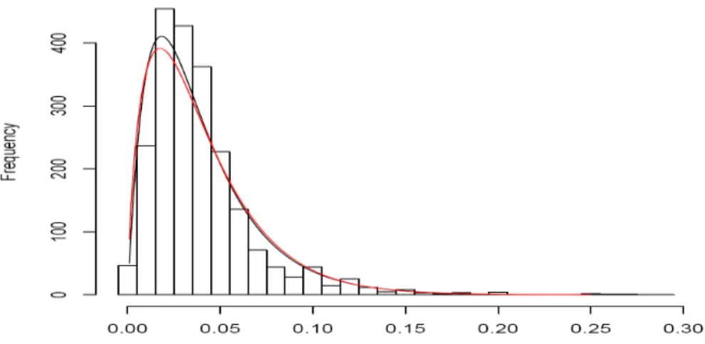
Figure 2: This …gure represents the distribution of the individual discount rates for the value = 0:4116 that maximizes the log-likelihood (upper curve) as well as the empirical distribution and Weitzman (2001)’s distribution (lower curve). Our distribution corresponds to the sum of two independent gamma distributions with parameters ( 1; 1) and ( 2; 2) given by ( 1; 1; 2; 2) = (1:04; 89:45; 1:04; 36:82) :

These parameters correspond to mean and variance levels given by (m1; v21; m2; v22) =

(1:16 10 2_{; 1:30 10} 4_{; 2:83 10} 2_{; 7:69 10} 4_{). Weitzman’s distribution}

cor-responds to a gamma distribution with parameters (1:78; 44:44): All represented distributions have the same mean and variance levels (m; v2) = (4 10 2; 9 10 4):

500 375 250 125 0 0.05 0.04 0.03 0.02 0.01 t r t r

Figure 3: This …gure represents the marginal discount rate curve rt =

PN i=1 wi iexp( rit) PN j=1wj jexp( rjt)r i ₌ 1+1 1+t+ 2

2+t obtained through our calibration (upper curve)

and compares it to the discount rate curve rt = _+t of Weitzman (2001) (lower

curve). The intermediate curve represents, with our calibration, the unweighted av-eragePN_i=1 wiexp( r

i_t) PN j=1wjexp( rjt) ri ₌ 1 1+t+ 2

2+t:It is clear that the di¤erence between our

discount rate curve and Weitzman (2001)’s curve mainly results from the fact that, contrarily to the certainty equivalent approach, more impatient experts are more heavily weighted in the equilibrium approach.

Time period Name Numerical value

Approx. rate

Weitzman’s

num. value Weitzman’sappr. rate Within years 1 to 5 hence Immediate Future 4.99% 5% 3.89% 4% Within years 6 to 25 hence Near Future 4.23% 4% 3.22% 3% Within years 26 to 75 hence Medium Future 2.82% 3% 2.00% 2% Within years 76 to 300 hence Distant Future 1.50% 1.5% 0.97% 1% Within years

more than 300 hence

Far-Distant

Future 0.16% 0% 0.08% 0%

Table 1 - Approximate recommended sliding-scale discount rates

This table compares for di¤erent time periods the recommended discount rates that result from our approach and those resulting from Weitzman (2001)’s approach. These rates are computed recursively. For the …rst period, we compute the rate that, if applied continuously from date 0 to the middle of the period would lead to the discount rate for that maturity. For next periods, we compute the rate that, if applied continuously from the beginning of the period to the middle of the period and compounded with the rates already computed for previous periods would lead to the discount rate for that maturity. The exact as well as approximate (recommended) results are then provided for both approaches.