Application de la méthode d'émission acoustique pour la surveillance du comportement au cisaillement des joints actifs

UNIVERSITE DE SHERBROOKE

Faculte de genie

Departement de genie civil

APPLICATION DE LA METHODE D'EMISSION

ACOUSTIQUE POUR LA SURVEILLANCE DU

COMPORTEMENT AU CISAILLEMENT DES

JOINTS ACTIFS

These de doctorat

Specialite: genie civil

Zabihallah MORADIAN

Jury: Gerard BALLIVY (directeur)

Patrice RIVARD

Giovanni GRASSELLI

Kaveh SALEH

Clermont GRAVEL

Mathieu NUTH

Library and Archives Canada Published Heritage Branch 395 Wellington Street Ottawa ON K1A 0N4 Canada Bibliotheque et Archives Canada Direction du Patrimoine de I'edition 395, rue Wellington Ottawa ON K1A 0N4 Canada

Your file Votre reference ISBN: 978-0-494-83299-8 Our file Notre reference ISBN: 978-0-494-83299-8

NOTICE:

The author has granted a

non-exclusive license allowing Library and Archives Canada to reproduce,

publish, archive, preserve, conserve, communicate to the public by

telecommunication or on the Internet, loan, distrbute and sell theses

worldwide, for commercial or non-commercial purposes, in microform, paper, electronic and/or any other formats.

AVIS:

L'auteur a accorde une licence non exclusive permettant a la Bibliotheque et Archives Canada de reproduire, publier, archiver, sauvegarder, conserver, transmettre au public par telecommunication ou par Plnternet, prdter, distribuer et vend re des theses partout dans le monde, a des fins commerciales ou autres, sur support microforme, papier, electronique et/ou autres formats.

The author retains copyright ownership and moral rights in this thesis. Neither the thesis nor substantial extracts from it may be printed or otherwise reproduced without the author's permission.

L'auteur conserve la propriete du droit d'auteur et des droits moraux qui protege cette these. Ni la these ni des extraits substantiels de celle-ci ne doivent etre imprimes ou autrement

reproduits sans son autorisation.

In compliance with the Canadian Privacy Act some supporting forms may have been removed from this thesis.

While these forms may be included in the document page count, their removal does not represent any loss of content from the thesis.

Conformement a la loi canadienne sur la protection de la vie privee, quelques formulaires secondares ont 6te enleves de cette these.

Bien que ces formulaires aient inclus dans la pagination, il n'y aura aucun contenu manquant.

Acknowledgement

Among many people who helped me to complete this thesis, first I want to express my sincere gratitude to my supervisor, Professor Gerard Ballivy at Universite de Sherbrooke, for his guidance throughout the duration of the study. I am greatly indebted for his support, advice, and suggestions to my research work. I would like to thank my co-supervisor, Professor Patrice Rivard, for his great assistance and his guidance during various parts of the work. Dr. Clermont Gravel has assisted me with many interesting discussions and comments. He is greatly acknowledged. I thank Dr. Serge Kodjo for his support and many inspirations and also for his useful comments.

I would like to express my thanks to Prof. Giovanni Grasselli, Dr. Kaveh Saleh and Prof. Mathieu Nuth for evaluating my thesis and giving their useful comments and suggestions. Gratitude is also expressed to those working at Laboratory of Rock Mechanics and Applied Geology, Civil Engineering Department, Universite de Sherbrooke especially, Georges Lalonde, Baptiste Rousseau and Danick Charbonneau who have helped me to carry out laboratory tests.

There are many colleagues and friends who deserve my sincere gratitude and acknowledgements. I thank all of them for their encouragement in various ways. I am so grateful that I have come to know and make friends with these wonderful People during my graduate study.

I want to thank my family and especially my parents, because their support has been invaluable. Finally, special thanks to my beloved wife who made this work possible with her patience and support.

Abstract:

A key requirement in evaluation of sliding stability of concrete dams is monitoring shear behavior of 1) concrete joints in dam body, 2) concrete-rock interfaces and 3) rock discontinuities in dam foundation. The methodology consisted of creating a database of observed shear behaviors of the mentioned joints using acoustic emission (AE) technique. Joint samples were fabricated by tension splitting of the cores and pouring concrete on rock joint replica for simulating concrete-rock interfaces. Variations of key parameters including joint geometry, normal stress, displacement rate and bonding percentage were incorporated in the analysis. An analysis was also carried out on natural joints from Daniel Johnson (Manic 5) Dam, Quebec, founded on gneiss to granitic rock. Parametric-based and signal-basedd analysis methods were used to evaluate the potential of AE for monitoring shear behavior of various kinds of joint with different characteristics. Using AE parameters such as amplitude, count, energy, duration and rise time, this study was done as a feasibility study for AE monitoring of sliding surfaces within dam, dam-rock interface or inside rock foundation. It was found that AE has a good capability for showing the initial shear movement of the non-bonded joints. For bonded joints this technique can show that AE activities are occurring before breaking of adhesive bond. This is important because recording AE signals after an initial breakage of the joint would be too late to install stabilization work to be done beforehand. Of course in the eventuality that a rupture includes a sequence of events even recording AE signals of the first break is still useful. It is recommended to use this method combined with other instrumentation methods (e.g. load measuring instruments) to detect the initial shear movement of the bonded joints. Following experimental work and analysis of crack propagation and asperity degradation along shearing process, four different periods were observed in shear stress-displacement behavior of joints. These periods are: 1) Pre-peak linear period in which AE activities are initiated and show the beginning of shear displacement, 2) Pre-peak non-linear period in which AE signals are generated from crack initiation and degradation of the secondary asperities, 3) Post-peak period where first order asperities are sheared off and joints pass their maximum shear strength and 4) Residual period in which AE activities decrease and reach their minimum values.

The applicability of AE localization technique was evaluated using image analysis and scanned surfaces of the joints by laser. The results indicated that this method can locate regions with rupture governing characteristics. This provides the possibility to reinforce support systems and be aware about possible structure failures before any unexpected mechanical disturbance.

Keywords: Acoustic emission; shear behavior; rock-rock joint; rock-concrete joint;

concrete-concrete joint; normal load; joint roughness; bonding percentage; displacement rate; AE parameters; AE source locations

Resume:

Une exigence cle dans 1'evaluation de la stabilite des barrages en beton est la surveillance du comportement au cisaillement des joints de beton dans le corps du barrage, des interfaces beton-roche et des discontinuites rocheuses dans les fondations du barrage. La methodologie propose dans cette etude consiste une base de donnees des comportements observes au cisaillement des joints du roc a l'aide de la technique d'emission acoustique (EA). Ces carottes de forage ont ensuite ete ruptures par flexion pour obtenir des repliques de joints rocheux. Un joint de beton a ensuite ete coule sur les surfaces des joints rocheux pour simuler les interfaces beton-roche. L'analyse a compris des variations des parametres cles, notamment la geometrie du joint, la contrainte normale, la vitesse de deplacement et le pourcentage de liaison. Une analyse a egalement ete effectuee sur des echantillons de joints naturels du barrage Daniel Johnson (Manic 5), Quebec, fondee sur le roc granitique. L'etude parametrique et celle sur les signaux ont ete utilisees pour evaluer le potentiel de TEA pour surveiller le comportement en cisaillement de differents types de joints possedant des caracteristiques differentes. Les parametres d'EA utilises ont ete l'amplitude, les comptes (counts), l'energie, la duration et le temps de montee. Cette etude a £te realisee comme une etude de faisabilite pour la surveillance de surfaces de glissement au sein d'un barrage : l'interface barrage-roche ou a l'interieur de la fondation rocheuse. II a ete constate que TEA a une bonne capacite a montrer le mouvement de cisaillement initial des joints non lies. Pour les joints lies, cette technique a demontre une activite d'EA un certain temps avant la rupture du lien adhesif. Ceci est important, puisqu'une fois le joint rompu, il serait trop tard pour installer des travaux correctifs. Bien sur, si une rupture se produit par une sequence d'evenements, dans ce cas, le signal d'emission acoustique de la premiere rupture est utile. II est recommande d'utiliser une combinaison de cette methode avec les methodes classiques d'instrumention et de mesure (par exemple, les instruments de mesure de la charge) pour detecter le mouvement de cisaillement initial des joints lies. A partir de l'estimation de la propagation des fissures et de la degradation des asperites pendant le processus de cisaillement, quatre periodes differentes ont ete observees dans le comportement contrainte-deplacement en cisaillement des joints. Ces periodes sont les suivantes: 1) periode prepic lineaire dans lequel les activites d'EA sont initiees et ou le point de depart du deplacement en cisaillement est montre, 2) periode prepic non lineaire dans lequel les signaux d'EA sont generes a partir du debut de la fissuration et de la degradation des asperites secondaire, 3) periode post-pic alors que les asperites de premier ordre sont arrachees et la resistance au cisaillement maximal est mobilisee par le joint et 4) periode residuelle dans lequel les activites d'EA sont diminuees et atteignent leur valeur minimale.

L'applicabilite de la technique de localisation d'EA a ete evaluee par analyse d'images et numerisation par profilometrie laser des surfaces des joints. Les resultats indiquent que cette methode peut reconnaitre les regions presentant des caracteristiques de rupture. Ceci offre la possibilite de renforcer des systemes de soutien de stuctures et de prevenir une rupture probable d'une structure suivant une perturbation mecanique inattendue.

Mots-cl6s: emission acoustique; comportement en cisaillement; joints roche-roche; joints

roche-beton; joints beton-beton; charge normale; rugosite du joint, pourcentage de liaison; vitesse de deplacement; parametres d'EA; localisation de sources d'EA

Table of Content

1. INTRODUCTION 1 1.1. Problem and rational 1 1.2. Discontinuities in dam structure 6

1.3. Acoustic emission monitoring 14 1.4. Objectives of the thesis 18 1.5. Originality of the thesis 18

1.6. Outline 20 2. STUDY ON THE CHARACTERISTIC FEATURES OF ACOUSTIC EMISSION

PARAMETERS DURING DIRECT SHEAR TEST OF ROCK JOINTS 23

2.1. Introduction 25 2.2. Methodology 27

2.2.1. Samples preparation and properties 27 2.2.2. Scanning the joint surface and determining the roughness values 28

2.2.3. Attaching the AE sensors and encapsulating the sample 29

2.3. Shear testing and detecting AE signals 30 2.4. Study AE parameters by applying constant normal load during whole period of direct

shear testing of the samples 33 2.5. Studying AE parameters by applying constant normal load in the beginning and

changing it in residual section of the same sample 42

2.6. Conclusions 48 3. EVALUATING DAMAGE DURING SHEAR TESTS OF ROCK JOINTS USING

ACOUSTIC EMISSIONS 50

3.1. Introduction 51 3.2. Sample preparation and testing 54

3.3. Predicting the start point of the shear movement by means of AE 58 3.4. Monitoring pre-peak, peak and post peak of shear strength graph by means of AE 63

3.4.1. Study on the basis of counts and energy rate 63 3.4.2. Study on the basis of cumulative count and energy 64

3.5. Discussion 69 3.6. Conclusions 74 4. APPLICATION OF ACOUSTIC EMISSION FOR MONITORING SHEAR BEHAVIOR

OF BONDED CONCRETE-ROCK JOINTS UNDER DIRECT SHEAR TEST 76

4.1. Introduction 78 4.2. Methodology 79 4.3. Shear mechanism of bonded concrete-rock joints 80

4.4. The effect of bonding percentage 84

4.5. The effect of normal load 89 4.6. The effect of the displacement rate 92

4.7. Conclusions 94 5. CORRELATING ACOUSTIC EMISSION SOURCES WITH DAMAGED ZONES.

DURING DIRECT SHEAR TEST OF ROCK JOINTS 95

5.1. Introduction 96 5.2. Scope of work 99 5.3. Experimental works 99

5.4. Calibrating AE source localization technique 101 5.5. Damaged zones and AE source locations 105

5.6. Discussion 118 5.7. Conclusions 119 6. CONCLUSIONS AND RECOMMENDATIONS 121

6.1. Conclusions francais 121 6.1.1. Les joints lies 123 6.1.2. Les joints non lies 123 6.1.3. L'effet du pourcentage de liaison 124

6.1.4. L'effet de la charge normale 125 6.1.5. Localisation des sources d'EA 126

6.2. Conclusions 128 6.2.1. Bonded joint samples 130

6.2.2. Non-bonded joint samples 130 6.2.3. The effect of bonding percentage 131

6.2.4. The effect of normal load 132 6.2.5. AE source locations 133 6.3. Recommendations 135

6.3.1. Using signal-based analysis of AE results for monitoring shear behavior of joints .135 6.3.2. Detailed analysis of combination of image processing, acoustic emission and scanned

surfaces using suitable softwares and instruments 136 6.3.3. 3D localization oftheAE source locations 136 6.3.4. AE monitoring of in situ discontinuities by applying in situ direct shear test 137

6.3.5. Borehole geophysical methods for knowing the real circumstances of the

discontinuities 137 APPENDIX 1: A FLOWCHART SHOWING METHODOLOGY STEPS 138

APPENDIX 2: PHOTOS SHOWING METHODOLOGY STEPS 140 APPENDIX 3: FIGURES SHOWING SHEAR AND AE BEHAVIORS OF MANIC 5

SAMPLES 165 REFERENCES 170

List of Figures

Figure 1-1: a concrete dam with various kinds of loads (after U.S. Army Corps of Engineers,

1995) 2 Figure 1-2: St. Francis dam before failure 3

Figure 1-3: St. Francis dam after failure 3 Figure 1-4: Malpasset Dam before failure 4 Figure 1-5: Maipasset Dam after failure 4 Figure 1-6: Looking from upstream, part of the wing wall remained on the left abutment 5

Figure 1-7: Almost nothing remained on the right abutment 5

Figure 1-8: Failure along concrete discontinuity 6 Figure 1-9: Failure along interface discontinuity 7 Figure 1-10: Failure along rock discontinuity 7 Figure 1-11: general shear stress versus shear displacement curves 8

Figure 1-12: First order and second order asperities, the main undulations are considered as first order asperities and the small teeth on these undulations are considered as second

order asperities 11 Figure 1-13: Constant normal load condition 13

Figure 1-14: Simulation of constant normal stiffness condition 13

Figure 1-15: Basic principle of Acoustic Emission 14 Figure 2-1: Common parameters of an AE waveform 26 Figure 2-2: Kreon Surface Profilometer Scanner 28

Figure 2-3: Zephyr sensor overview 28 Figure 2-4: Diagram of vertical section through shear apparatus 31

Figure 2-5: PAC AE system - u-SAMOS 32 Figure 2-6: shear stress vs. shear displacement 34 Figure 2-7: Normal displacement vs. shear displacement 34

Figure 2-8: On the left, shear stress and rate of AE parameters vs. shear displacement and on the right shear stress and cumulative AE parameters vs. shear displacement for sample

number 44 under normal stress=0.5 MPa 36 Figure 2-9: On the left, shear stress and rate of AE parameters vs. shear displacement and on

the right, shear stress and cumulative AE parameters vs. shear displacement for sample

number 25 under normal stress=l MPa 38 Figure 2-10: On the left Shear stress and rate of AE parameters vs. shear displacement and on

the right shear stress and cumulative AE parameters vs. shear displacement for sample

number 15 under normal stress =2 MPa 40 Figure 2-11: Shear stress and normal displacement vs. shear displacement for sample number

33, 1) normal stress=0.5 MPa, 2) normal stress=l MPa, 3) normal stress=2 MPa, 4)

normal stress=l MPa, 5) normal stress=0.5 MPa 43 Figure 2-12: Shear stress and normal displacement vs. shear displacement for sample number

34, 1) normal stress=2 MPa, 2) normal stress=1.5 MPa, 3) normal stress=0.5 MPa, 4)

normal stress=1.5 MPa, 5) normal stress=2 MPa 44 Figure 2-13: On the left, shear stress and rate of AE parameters vs. shear displacement and on

the right, shear stress and cumulative AE parameters vs. shear displacement for sample

number 33 under normal stresses shown in Figure 2-11 45

Figure 2-14: On the left, shear stress and rate of AE parameters vs. shear displacement and on the right, shear stress and cumulative AE parameters vs. shear displacement for sample

number 34 under normal stresses shown in Figure 2-12 47 Figure 3-1: Shear stress vs. shear displacement: (a) bonded concrete-concrete joint (sample

BCC3.45), (b) non-bonded concrete-concrete joint (sample CC8.35), (c) non-bonded rock-concrete joint (sample RC7.63) and (d) non-bonded rock-rock joint (sample

RR10.48) 55 Figure 3-2: Normal displacement vs. shear displacement: (a) bonded concrete-concrete joint

(sample BCC3.45), (b) bonded concrete-concrete joint (sample CC8.35), (c) non-bonded rock-concrete joint (sample RC7.63) and (d) non-non-bonded rock-rock joint (sample

RR10.48) 56 Figure 3-3: Shear stress and count rate vs. time: (a) bonded concrete-concrete joint (sample

. BCC3.45), (b) non-bonded concrete-concrete joint (sample CC8.35), (c) non-bonded rock-concrete joint (sample RC7.63) and (d) non-bonded rock-rock joint (sample

RR10.48) 60 Figure 3-4: Shear stress and energy rate vs. time: (a) bonded concrete-concrete joint (sample

BCC3.45), (b) non-bonded concrete-concrete joint (sample CC8.35), (c) non-bonded rock-concrete joint (sample RC7.63) and (d) non-bonded rock-rock joint (sample

RR10.48) 62 Figure 3-5: Shear stress and cumulative count vs. time: (a) bonded concrete-concrete joint

(sample BCC3.45), (b) bonded concrete-concrete joint (sample CC8.35), (c) non-bonded rock-concrete joint (sample RC7.63) and (d) non-non-bonded rock-rock joint (sample

RR10.48) 66 Figure 3-6: Shear stress and cumulative energy vs. time: (a) bonded concrete-concrete joint

(sample BCC3.45), (b) bonded concrete-concrete joint (sample CC8.35), (c) non-bonded rock-concrete joint (sample RC7.63) and (d) non-non-bonded rock-rock joint (sample

RR10.48) 68 Figure 3-7: A 3D view of lower and upper surfaces of non-bonded concrete-concrete joint

(sample CC8.35) 70 Figure 3-8: A profile drawn at middle of lower and upper surfaces of non-bonded

concrete-concrete joint in the direction of shearing (sample CC8.35) 70 Figure 3-9: A 3D view of lower and upper surfaces of non-bonded rock-concrete joint (sample

RC7.63) 71 Figure 3-10: A profile drawn at middle of lower and upper surfaces of non-bonded

rock-concrete joint in the direction of shearing (sample RC7.63) 71 Figure 3-11: A 3D view of lower and upper surfaces of non-bonded rock-rock joint (sample

RR10.48) 72 Figure 3-12: A profile drawn at middle of lower and upper surfaces of non-bonded rock-rock

joint in the direction of shearing (sample RR10.48) 72 Figure 4-1: Four detected periods in shear behavior of a bonded concrete-rock joint under

normal stress of 0.25 MPa a) shear stress and AE energy rate vs. shear displacement, b)shear stress and cumulative AE energy vs. shear displacement, a and b') are a close-up

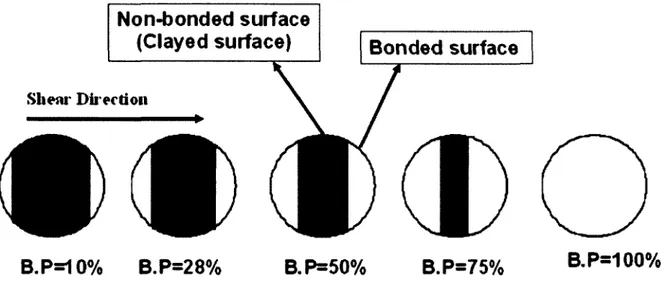
of the graphs a and b for lmmof shear displacement 82 Figure 4-2: Normal displacement vs. shear displacement 83 Figure 4-3: Schematic plans showing the bonding percentages of the joint samples 84

Figure 4-5: Maximum shear strength vs. bonding percentage 87 Figure 4-6: Max. AE energy rate at the peak vs. bonding percentage 87

Figure 4-7: Cumulative AE energy vs. bonding percentage 88 Figure 4-8: Shear stress and a) AE energy rate b) Cumulative AE energy vs. shear

displacement for samples under different values of normal load 91 Figure 4-9: Shear stress and a) AE energy rate b) Cumulative AE energy vs. shear

displacement for various displacement rates 93 Figure 5-1: An array of the AE transducers around an AE source (after Hardy, 2003) 98

Figure 5-2: a) A 25.5 ><28 x 8 cm mortar slab and attached sensors, b) localizing AE events by tapping central point of the slab. Black points in the 2D location graph show the position

of the sensors 102 Figure 5-3: a) A 10 ><20 x 5.5 cm granite slab and attached sensors, b) localizing AE events

by tapping central point of the slab. Black points in the 2D location graph show the

position of the sensors 103 Figure 5-4: a) A 25.5 ><28 x 6.5 cm concrete slab and attached sensors, b) localizing AE

events by tapping central point of the slab. Black points in the 2D location graph show

the position of the sensors 104 Figure 5-5: Shear stress vs. shear displacement of the rock joint samples 107

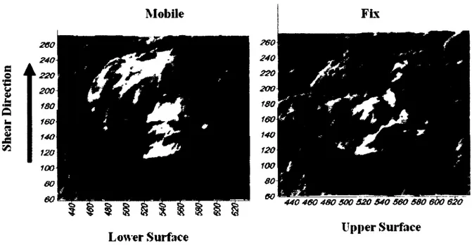
Figure 5-6: 2D source location of the AE events and their corresponding energy in X and Y directions for the mobile surface of the sample number 44 under normal stress of 0.5 MPa. Black points in the 2D location graphs show the position of the sensors. The arrow shows the shear direction and the photo shows the top view picture of the mobile surface after

shear test 109 Figure 5-7: 2D source location of the AE events and their corresponding energy in X and Y

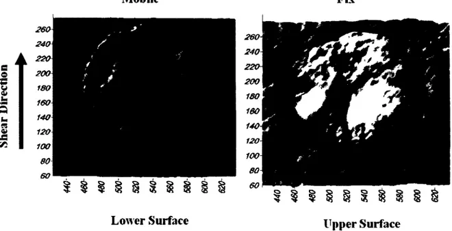
directions for the mobile surface of the sample number 25 under normal stress 1 MPa. Black points in the 2D location graphs show the position of the sensors. The arrow shows the shear direction and the photo shows the top view picture of the mobile surface after

shear test I l l Figure 5-8: 2D source location of the AE events and their corresponding energy in X and Y

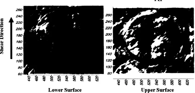
directions for the mobile surface of the sample number 15 under normal stress 2 MPa. Black points in the 2D location graphs show the position of the sensors. The arrow shows the shear direction and the photo shows the top view picture of the mobile surface after

shear test 113 Figure 5-9: Top view picture of the mobile surface after shear test, sample number 44 under

Normal stress=0.5 MPa. Picture belongs to mobile replica which the AE sensors were attached to. The arrow shows the shear direction. In the top and left side of the figure, the central 2D profile of the surface roughness drawn in X and Y directions have been shown.

115 Figure 5-10: Top view picture of the mobile surface after shear test, sample number 25 under

Normal stress=l MPa. Picture belongs to mobile replica which the AE sensors were attached to. The arrow shows the shear direction. In the top and left side of the figure, the central 2D profile of the surface roughness drawn in X and Y directions have been shown.

116 Figure 5-11: Top view picture of the mobile surface after shear test, sample number 15 under

Normal stress =2 MPa. Picture belongs to mobile replica which the AE sensors were attached to. The arrow shows the shear direction. In the top and left side of the figure, the

central 2D profile of the surface roughness drawn in X and Y directions have been shown. 117

Figure Al- 1: Program of laboratory tests 139

Figure A2- 1: Coring rock samples from a granite block 141 Figure A2- 2: Tension splitting of the rock cores to create a jointed sample 142

Figure A2- 3: Rock replicas ready for pouring mortar in order to create bonded rock-concrete

joints ; 143 Figure A2- 4: Spreading clay to create bonded rock-concrete joints with different amounts of

bonding percentage 144 Figure A2- 5: A rock-rock joint sprayed by a blue color ready for shear testing and

localization ofthe AE sources 145 Figure A2- 6: A prepared bonded rock-concrete joint 146

Figure A2- 7: Subbing sensor positions by a rotary sander 147 Figure A2- 8: A core drilled from Manic 5 dam containing a rock-rock joint 148

Figure A2- 9: A core drilled from Manic 5 dam containing a concrete-rock joint 149 Figure A2- 10: A core drilled from Manic 5 dam containing a concrete-concrete joint 150 Figure A2-11: Mobile part of shear test mold ready for encapsulating a sample 151 Figure A2- 12: Joint sample positioned in the mold considering the shear direction and

horizontal level of the joint surface 152 Figure A2- 13: Pouring Ciment Sika Grout 212 with E/C=0.18, before pouring the sensor

positions were kept by fixing a fiber piece between each sensor position and the wall of

the mould 153 Figure A2- 14: Pouring Ciment Set 45 with E/C=0.08 which is cured very fast and fixes the

sample perfectly in the mold 154 Figure A2- 15: Putting sensors in the considered holes and attaching them to the sample using

Loctite Metal/Concrete Epoxy (01-81508) glue 155 Figure A2- 16: Smooth clay is used to separate the two halves of mold and prevents grout to

inter into area between joint surfaces during grouting second mold. The clay covers the

sensors and makes a good ambient for shearing ofthe surfaces 156 Figure A2- 17: Putting the Fix half of the mould on the mobile half 157

Figure A2- 18: Encapsulating the whole mold 158 Figure A2- 19: Mounting mold in the MTS loading system and connecting sensors to the

amplifiers and AE PAC system 159 Figure A2- 20: Amplifiers used in this study (preamplifier model 2/4/6 with 10 KHz - 1200

KHz bandpass filter) 160 Figure A2- 21: Fixed half of the joint sample after shear test 161 Figure A2- 22: Mobile half of a rock-rock joint with light colored zones which are showing

the asperity damaged zones 162 Figure A2- 23: Fixed half of previous rock-rock joint with light colored zones which are

showing the asperity damaged zones 163 Figure A2- 24: A rock-concrete joint sample after direct shear test, the asperity damaged

Figure A3- 1: a) Shear stress and normal displacement vs. shear displacement, b) shear stress and AE count rate vs. shear displacement, c) shear stress and AE energy rate vs. shear displacement, d) shear stress and cumulative AE count rate vs. shear displacement and e) shear stress and cumulative AE energy rate vs. shear displacement for non-bonded

rock-rock joint (Sample MC6-RR10) 166 Figure A3- 2: a) Shear stress and normal displacement vs. shear displacement, b) shear stress

and AE count rate vs. shear displacement, c) shear stress and AE energy rate vs. shear displacement, d) shear stress and cumulative AE count rate vs. shear displacement and e) shear stress and cumulative AE energy rate vs. shear displacement for non-bonded

rock-concrete joint (Sample MC6-RC5.36) 167 Figure A3- 3: a) Shear stress and normal displacement vs. shear displacement, b) shear stress

and AE count rate vs. shear displacement, c) shear stress and AE energy rate vs. shear displacement, d) shear stress and cumulative AE count rate vs. shear displacement and e) shear stress and cumulative AE energy rate vs. shear displacement for non-bonded

concrete-concrete joint (Sample MC6-CC2.18) 168 Figure A3- 4: a) Shear stress and normal displacement vs. shear displacement, b) shear stress

and AE count rate vs. shear displacement, c) shear stress and AE energy rate vs. shear displacement, d) shear stress and cumulative AE count rate vs. shear displacement and e) shear stress and cumulative AE energy rate vs. shear displacement for bounded

concrete-concrete joint (Sample MC6-CC6.60) 169

List of Tables

Table 1-1: Characteristics of acoustic emission method compared with other NDT methods.... 16

Table 1-2: Non-bonded rock-rock joints used in chapter 2 and 5 21 Table 1-3: Bonded concrete-rock joints used in chapter 3 for study the effect of normal load ....21

Table 1-4: Bonded concrete-rock joints used in chapter 3 for study the effect of

displacement rate 21 Table 1-5: Bonded concrete-rock joints used in chapter 3 for study the effect of

bonding percentage 21 Table 1-6: List of natural samples cored from Manic 5 dam and used in chapter 3 22

Table 2-1: Physical and mechanical properties ofthe granite rock cores 27 Table 2-2: Technical Characteristics ofthe Zephyr Sensor Range: KZ25 29

Table 2-3: Surface roughness parameters ofthe joint samples 29 Table 2-4: characteristics of AE sensors used in this study 32 Table 2-5: Characteristics of AE parameters under different values of normal load 41

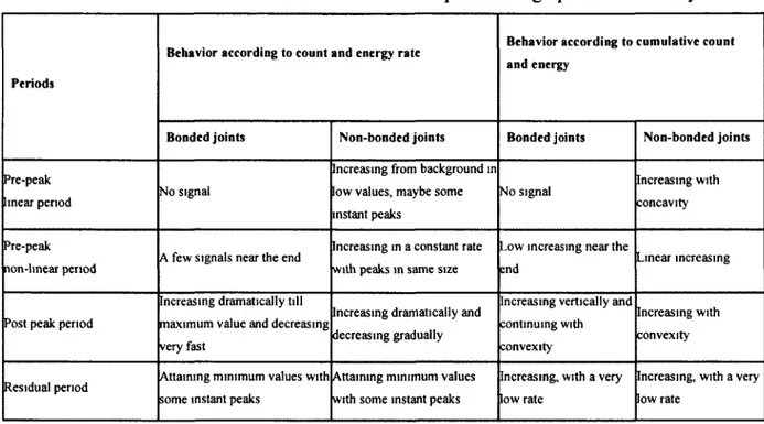
Table 3-1: Z2 parameter for each sample 57 Table 3-2: Different behaviors in shear stress-shear displacement graphs monitored by AE 75

Table 4-1: The mixture recipe for 90 kg mortar 80 Table 4-2: Physical and mechanical properties ofthe rock and concrete replicas 80

Table 4-3: Shear strength and AE results ofthe samples under different values of bonding

percentage 87 Table 4-4: Shear strength and AE results ofthe samples under different values of normal load .90

Table 4-5: Shear strength and AE results ofthe samples under different values of displacement

rate 92 Table 5-1: Physical and mechanical properties ofthe granite rock cores 100

1. INTRODUCTION

1.1. Problem and rational

Since the early part of 20th century, and especially since the 1950s, the number of hydroelectric dams has increased across the Canadian landscape. The province of Quebec has based a large part of its economic growth and activities in the energy sector on the development of the extensive water resources found throughout its territory. Quebec is Canada's leading producer of hydroelectricity. It also has one of the world's largest hydroelectric facilities with more than 568 dams. Hydroelectricity, with 34 GW potential, accounts for almost 96% of all the electricity used in Quebec (Hydro-Quebec, 2010).

Over the past few years, the monitoring of dams in Canada and especially in Quebec has acquired great importance not only for dam managers but also for scientific communities. Dam monitoring helps to understand the mechanisms of disruptive processes and define adequate prevention measures for the mitigation of their effects and reduce the loss of human lives and assets.

Concrete dams deform due to internal loads such as dead load, pore pressure, cooling, alkali-aggregate reaction in concrete, etc, external loads caused by weather and reservoir temperature, solar radiation, reservoir levels, uplift pressure, wind, earthquakes, ice, overflowing water, foundation settlement, etc. Figure 1-1 shows a typical concrete dam with various kinds of loads.

Movements caused by such loads must be within the tolerable ranges and do not cause structural distress. Sudden or unexpected direction or trend of surface movement could indicate developing problems.

The causes of dam failures and incidents have been catalogued (USCOLD 1975, 1988 and 1996 and ICOLD 1973, 1976, 1979 and 1995). The common causes of concrete dam failures and incidents are (ICOLD 1973):

• Overtopping from inadequate spillway capacity or spillway blockage resulting in erosion ofthe foundation at the toe ofthe dam or washout of an abutment or adjacent embankment structure.

Foundation leakage and piping in pervious strata, soluble lenses, and rock discontinuities which accelerate the rupture/collapse of the structure.

Sliding along weak discontinuities in foundations.

Ice pressure Dead load Hydrostatic pressure /—*-Alkali-aggregate reaction Uplift pressure

! f f t i J

Figure 1-1: a concrete dam with various kinds of loads (after U.S. Army Corps of Engineers, 1995)

One example of dam failure due to sliding is St. Francis dam in USA. On March 12, 1928, the St. Francis dam catastrophically failed. Approximately 450 people lost their lives in the downstream zones. Among those that died, were many of the workers and their families that worked at the dam. The St. Francis Dam Failure is considered the greatest American civil engineering failure of the twentieth century (Doyce and Nunis, 2002). Figure 1-2 and 1-3 show the ST. Francis dam before and after failure.

Figure 1-2: St. Francis dam before failure

Figure 1-3: St. Francis dam after failure

Another famous concrete dam failure was Malpasset Dam in France. The dam was a double curvature arch dam of 66.5 m maximum height, with a crest length of 223 m. The dam failed explosively on 2nd December 1959. A total of 433 casualties were reported (Goutal, 1999). Investigations after the accident showed that the key factors in the failure of the dam were the pore water pressure in the rock, and the nature of the rock. Under the increasing pressure of rising water, the arch separated from its foundation and rotated as a whole about its upper right end. The whole left side of the dam collapsed, followed by the middle part, and then the right

supports (Goutal, 1999). Figure 1-4 shows the Malpasset dam before failure. Figure 1-5 to 1-7 show the Malpasset dam after failure.

Figure 1-4: Malpasset Dam before failure

Figure 1-6: Looking from upstream, part ofthe wing wall remained on the left abutment

Figure 1-7: Almost nothing remained on the right abutment

But could failure have been avoided if the cracking had been investigated? This is one of the most important lessons learnt from the Malpasset dam failure that is taken very seriously today.

It can be noted that the use of adequate monitoring systems is a powerful tool for understanding kinematic aspects of mass movements and permits their correct analysis and interpretation; in addition, it is an essential aid in identifying and checking alarm situations.

Dams with complex foundations, known geologic anomalies, marginal design criteria, or unconservative assumptions usually require more instrumentation to demonstrate satisfactory performance than dams without those features. Collapses of dam structures such as Malpasset dam have demonstrated once again the need for a reliable tool for an early monitoring of damage progression.

1.2. Discontinuities in dam structure

Discontinuities play an important role in the behavior of dam under normal and shear loading conditions. They cause reduction of strength and increase of deformability in dam structures. Thus the safe management of dam operation requires a precise evaluation of the dam stability in terms of the shear strength of the concrete-rock contact, a concrete lift joint or a discontinuity in the rock mass. Figures 1-8 to 1-10 show the three kinds of failure in dam caused by discontinuities.

Upstream

.XZ

Downstream

Figure 1-9: Failure along interface discontinuity (after U.S. Army Corps of Engineers, 1994)

Upstream _Downstream

Figure 1-10: Failure along rock discontinuity (after U.S. Army Corps of Engineers, 1994)

The appropriate definition of failure generally depends on the shape (envelope) of the shear stress versus shear deformation/strain as well as the mode of potential failure. Regardless of the mode of potential failure, the selection of shear strength parameters for use in the design process invariably involves the testing of appropriate specimens. Selection of the type of test best suited for intact or discontinuous structure, as well as selection of design shear strength parameters, requires an appreciation of joint failure characteristics (U.S. Army Corps of

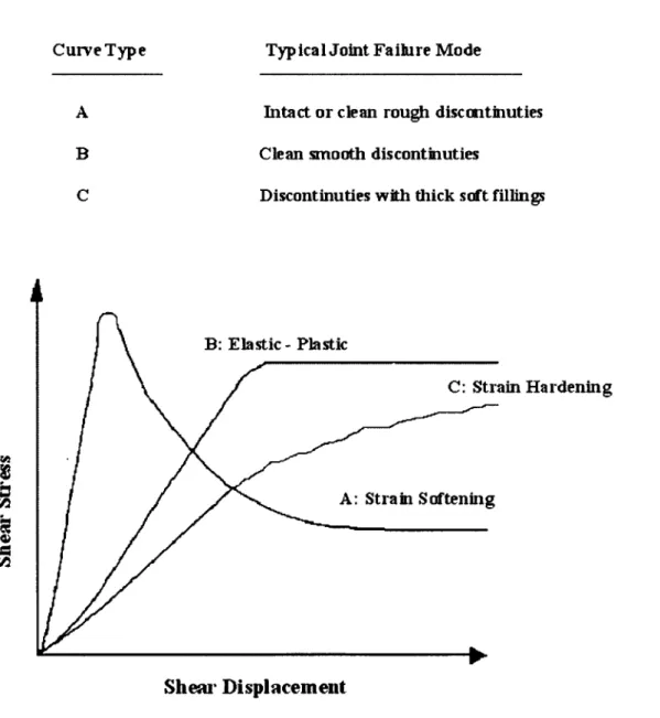
Engineers, 1994). Figure 1-11 illustrates three general shear stress-deformation curves commonly associated with joint failure.

The typical failure envelope for a clean discontinuity is curvilinear. At stress levels associated with low head gravity dams, retaining walls and slopes, almost all joints behave in a strain softening manner at failure. Strain softening failure is specified by a rapid increase in applied stress, with small strains, until a peak stress is obtained. Further increases in strain causes a rapid drop off in stress and then the residual stress value is reached.

CurveType TypicalJoint Failure Mode

A B C

Intact or clean rough discontinuties Clean smooth discontinuties

Discontinutles with thick soft fillings

8 5=

1 \ B:

•

Mohr-Coulomb equation is one ofthe first equations representing the relationship between the peak shear strength T and the normal stress a :

p n

Tp=c + <7ntm</> (1-1)

Where c is the cohesive strength ofthe cemented surface and <f> is the angle of friction. In the case of the residual strength, the cohesion c has dropped to zero and Mohr-Coulomb equation is represented by:

Tp= crn t a n <f>r (1-2)

Where ^ is the residual angle of friction.

A natural discontinuity surface in hard rock is never as smooth as a sawn or ground surface. The undulations and asperities on a natural joint surface have a significant influence on its shear behaviour. Generally, this surface roughness increases the shear strength of the surface, and this strength increase is extremely important in terms of the stability of excavations in rock.

Patton (1966) demonstrated this influence by means of an experiment in which he carried out shear tests on saw-tooth specimens.

Shear displacement in these specimens occurs as a result of the surfaces moving up the inclined faces, causing dilation (an increase in volume) of the specimen. The shear strength of Patton's saw-tooth specimens can be represented by:

rp= o - „ t a n ( ^ + 0 (1-3)

Where <f>b is the basic friction angle ofthe surface and / is the angle ofthe saw-tooth face.

Equation (1-3) is valid at low normal stresses where shear displacement is due to sliding along the inclined surfaces. At higher normal stresses, the strength of the intact material will be exceeded and the teeth will tend to break off, resulting in a shear strength behaviour that is more closely related to the intact material strength than to the frictional characteristics of the surfaces.

While Patton's approach has the merit of being very simple, it does not reflect the reality that changes in shear strength with increasing normal stress are gradual rather than abrupt.

Ladanyi and Archambault (1970) suggested the shear strength ofthe material adjacent to the discontinuity surfaces:

. _ g , ( i -

X r + 7 W ) + g , . T , 0-

)

l-(JL-at)VTanfa

where T is joint shear strength, <f>B is basic friction angle, as is the proportion of the

discontinuity surface which is sheared through projections of intact material, V is the dilation rate (dv/du) at peak shear strength, and xt is the shear strength ofthe intact material.

They defined as to be the area where shearing through the asperities takes place. Over the rest ofthe surface, 1 - as, the asperities are assumed to slide over each other without damage.

Barton (1973) studied the behaviour of natural rock joints and has proposed this equation:

rp = <r„ tan(fc + JRClogl0(—) ( 1"5 )

0-*

Where JRC is the Joint Roughness Coefficient and JCS is the Joint Wall Compressive Strength.

Surfaces of discontinuous rock are composed of irregularities or asperities ranging in roughness from almost smooth to sharply inclined peaks. Conceptually there are three modes of failure: asperity override at low normal stresses (sliding process), failure through asperities at high normal stresses (shearing process), and a combination of asperity override and failure through asperities at intermediate normal stresses.

Patton (1966) recognized that the asperity of a rough joint occurs on many scales. He first categorized asperity into first-order (waviness) and second-order (unevenness) categories. The behavior of rock joints is controlled primarily by the second-order asperity during small displacements and the first-order asperity governs the shearing behavior for large displacements. Barton (1973) and Hoek and Bray (1981) also stated that at low normal stress levels the second-order asperity (with higher-angle and narrow base length) controls the shearing process. As the normal stress increases, the second-order asperity is sheared off and the first-order asperity (with longer base length and lower-angle) takes over as the controlling factor.

As indicated in Figure 1-12, first-order irregularities generally have smaller angles of inclination than second-order irregularities.

First order asperities Second order asperities

Figure 1-12: First order and second order asperities, the main undulations are considered as first order asperities and the small teeth on these undulations are considered as second order asperities

It is recognized that a precise measurement of the rough surface topography is necessary to study the shearing mechanism and predict the peak and residual strength of rock joints, as well as the amount of dilatation a discontinuity undergoes during shearing.

The joint roughness coefficient (JRC) proposed by Barton (1973), has been widely used in engineering practice. The JRC value scales the joint roughness in the range from 20 (rough) to 0 (smooth) and can be determined by various methods.

The JRC can be estimated by comparing the appearance of a discontinuity surface with standard profiles published by Barton and others. One of the most useful of these profile sets was published by Barton and Choubey (1977).

The appearance of the discontinuity surface is compared visually with the profiles shown and the JRC value corresponding to the profile which most closely matches that of the discontinuity surface is chosen. In the case of small scale laboratory specimens, the scale of the surface roughness will be approximately the same as that of the profiles illustrated. However, in the field the length of the surface of interest may be several meters or even tens of meters and the JRC value must be estimated for the full scale surface.

On the basis of extensive testing of joints, joint replicas, and a review of literature, Barton and Bandis (1982) proposed the scale corrections for JRC defined by the following relationship:

JRC. = JRQ

( T \

\L0j _(1-6)

Where JRCo, and Lo refer to 100 mm laboratory scale samples and JRCn, and Ln refer to in situ sizes.

Many researchers have also investigated the applicability of various conventional statistical parameters for calculating the JRC. Tse and Cruden (1979) found that among eight different statistical parameters, two parameters, Z2 (the slope of asperity) and SF (structure function) are strongly correlated with the values of JRC.

JRC0 = 32.2 + 32.47 log(Z2) (1-7)

JRC=7.14961n(SF)+37.014 (1-8) Detailed laboratory investigations, however, indicated that JRC varies not only from fracture

to fracture but also with scale. The limitation of JRC and the conventional statistical parameters in quantifying joint roughness have also been reported by Kulatilake et al (1995). Therefore, surface roughness of rock joints need to be characterized using a scale-invariant parameter.

In recent years, because ofthe pioneering work of Mandelbrot (1983) on fractal geometry, there have been a number of studies to investigate the applicability of fractal models to characterize roughness of fracture surface. The attraction of a fractal model lies in its ability to predict scaling behavior, i.e., the relationship between surface geometry observed at different scales.

Assuming the rock surface profiles are self-similar fractals, researchers such as Carr and Warriner (1989), Lee et al. (1990), and Wakabayashi and Fukushige (1992) have developed relations between the fractal dimension D and the JRC0. The relations are as follows:

Carr and Warriner (1989):

JRC0 =-1022.55 + 1223.92D (1-9)

Lee etal., (1990):

JRC, = -0.8780 + 3 7 . 7 8 4 4 ( - ^ - ) - 1 6 . 9 3 0 4 ( - ^ i )2

0 0.015 0.015 (!_!())

Wakabayashi and Fukushige (1992):

JRC

~

capture the features necessary for characterising three dimensional (3D) roughness strength (Grasselli et al, 2002). Recently researchers have focused their attention on identifying 3D parameters to quantify the relationship between the surface roughness and shear strength (Gentier and Hopkins, 1997, Lanaro et al, 1998, Grasselli et al. 2002).

Generally, shearing of joints occurs in situ under a variety of boundary conditions. However, it is possible to identify two different characteristic behaviors: the first condition, where a rock block slides down a rock slope, the normal load acting on the joint surface remains constant during the shearing process. In this case, shearing occurs under a constant normal load (CNL, free dilation) condition. Figure 1-13 shows this boundary condition.

i

Figure 1-13: Constant normal load condition (after Brady and Brown, 2005)

The second condition, where a block on the roof or the sidewalls of an underground excavation is extruded into the opening, the normal load on the joint surface is no longer constant, but continuously evolved due to the restriction on the normal dilation (figure 1-14).

no normal

displacement permitted

Figure 1-14: Simulation of constant normal stiffness condition (after Brady and Brown, 2005)

Nevertheless, the mechanical behavior of shear tests made under constant normal load (CNL) or constant normal stiffness (CNS) conditions differs only after the peak, when dilation plays an important role, inducing an increment in the normal stress. This increment is proportional to the stiffness of the rock. Before reaching the peak, since very little or no dilation has occurred, both types of shear tests follow the same path (Ohnishi and Dharmaratne 1990, Skinas et al 1990 and Olsson and Barton 2001).

For studying the joint behavior in dam body and under the foundations of dams, it can be assumed that the high water pressure against the face of the dam produces shearing along fractures. Depending on the orientations of the joint sets and their depth, each joint can dilate freely under a normal load in the range of 0.2- 5.0MPa. Therefore for these situations, the most appropriate laboratory experimental shear test set-up is the CNL condition (Grasselli, 2001).

1.3. Acoustic emission monitoring

Acoustic Emissions are stress waves produced by sudden movement in stressed materials. The classic sources of acoustic emissions are defect-related deformation processes such as crack initiation and crack propagation. The process of generation and detection is illustrated in Figure 1-15. AE Transducer Prc-Amplifier

o-yv

Sudden movement at the source produces a stress wave, which radiates out into the structure and excites a sensitive piezoelectric transducer. As the stress in the material is raised, many of these emissions are generated. The signals from one or more sensors are amplified and measured to produce data for display and interpretation.

Without stress, there is no emission. Therefore, an acoustic emission (AE) inspection is usually carried out during a controlled loading ofthe structure. This can be a proof load before service, a controlled variation of load while the structure is in service, a fatigue test, a creep test, or a complex loading program. Often, a structure is going to be loaded anyway, and AE inspection is used because it gives valuable additional information about the performance of the structure under load. Other times, AE inspection is selected for reasons of economy or safety, and a special loading procedure is arranged to meet the needs of the AE test (Pollock, 2005).

In geologic material, the origin of AE activity appears to be related to processes of deformation and failure which are accompanied by a sudden release of energy. In such materials, which are basically polycrystalline in nature, AE activity may originate at the micro level as a result of dislocations, at the macro level by twining, grain boundary movement, or initiation and propagation of fractures through and between mineral grains and at the mega level by fracturing and failure of large areas of material or relative motion between structural units (Hardy, 2003).

Acoustic emission differs from most other nondestructive testing (NDT) methods in two key respects. First, the signal has its origin in the material itself, not in an external source. Second, acoustic emission detects movement or crack propagation, while most other methods detect existing geometrical discontinuities. The consequences of these fundamental differences are summarized in Table 1 -1.

Table 1-1: Characteristics of acoustic emission method compared with other NDT methods (after Pollock, 2005)

Acoustic Emission

Detects movement of defects Requires stress

Each loading is unique More material-sensitive Less geometry-sensitive Less intrusive on plant/process Requires access only at sensors Tests whole structure at once Main problems: noise related

Other NDT Methods

Detect geometric form of defects Do not require stress

Inspection is directly repeatable Less material-sensitive

More geometry-sensitive More intrusive on plant/process

Requires access to whole area of inspection Scan local regions in sequence

Main problems: geometry related

Precautions must be taken into account against interfering noise as an important part of AE technology. The first point is selection of an appropriate frequency range for AE monitoring. The acoustic noise background is highest at low frequencies. On the other hand because higher frequencies bring reduced detection range, there is an inherent trade-off between detection range and noise elimination (Pollock, 2005). The frequencies of interest for field and laboratory studies in the general geotechnical area (i.e., rock and soil mechanics) extend over a wide central region ofthe overall frequency rage (10°<f<5 * 10s Hz). It is clear, therefore, that

AE studies in the geotechnical filed overlap at low frequencies with seismology, and at high frequencies with material science related AE studies (Hardy, 2003).

Noises can be stopped at the source. Applying impedance mismatch barriers or damping materials at strategic points on the structure is another way to eliminate an acoustic noise. Differential sensors or sensors with built-in preamplifiers are useful for eliminating electrical noise problems which are often the result of poor grounding and shielding practices. If noises can not be omitted through hardware setup, the problem must be dealt with by software setting in the AE instrument. One of the effective ways is sensitivity adjustments including fixed and floating threshold techniques. Signal filtering for selective acceptance and recording of data based on time, load, or spatial origin are very useful for collecting agreeable signals. Moreover,

because noise sources often give characteristically different waveforms, advanced waveform analysis package can help us to differentiate noises from AE signals (Pollock, 2005).

Interesting aspects for acoustic emission are the monitoring of damage development in critical parts of a structure. Compared to other active ultrasonic methods that assess mainly the structure itself or existing failures, the power of AE analysis is the possibility to directly observe the process of deterioration. With AE analysis spatial and temporal correlations are examined. One aspect of monitoring a stressed structure is to localize AE sources and, in this way, to observe the region where damage takes place. On the other hand, investigation of the AE activity in terms of signal rate or event magnitude distribution could indicate the stage of damage progress. The aim is to obtain reliable relations that can be applied during the AE monitoring for condition assessment of the structural component. This way of data analysis could contribute to an early warning (alarm) system that is able to detect precursors of a soon failure.

When joints (construction joints in concrete, concrete-rock interfaces and rock joints in foundation) are under loading, once a critical state of shear stress is reached, a certain part of the joint is deformed. The identification of this predisposed stage before total failure is important to reduce the danger of sudden release of deformation energy. This prevention process can be done by AE monitoring.

Over the past few decades parameter-based and signal-based acoustic emission (AE) techniques were developed into a sophisticated tool for non-destructive testing of several materials.

Parameter-based AE techniques identify AE wave packets searching for particular parameters. The essential parameters for interpretation such as hits, amplitude and wave energy can be used with their occurrence rate or their accumulated trend in the time domain (Grosse 2007). Wave amplitudes exceeding a defined threshold value are referred to as AE events. Signals below the threshold value are considered as noise. Signal-based AE techniques consider the complete waveform. Typically, a waveform consists of a compression or primary wave (P-wave), a shear or secondary wave (S-wave) and surface waves. The arrival time (onset time) of the P-wave of each event can be determined (picked) and used to localize the respective source (Kurz et al. 2005).

1.4. Objectives ofthe thesis

The main objective of this research is to evaluate the application of acoustic emission for monitoring shear behavior of joint in laboratory as a feasibility study for monitoring shear behavior of active joints in dam body, interface joint between dam body and rock mass and rock joints in dam foundation. In fact simulating various kinds of joints with different characteristics and correlating AE and shear test results in laboratory helps us to have a better interpretation of shear process ofthe in situ discontinuities.

• A methodology for detecting and interpreting the AE signals during direct shear test of joints is developed. In this methodology, sample preparation, testing procedure, AE set up,

recommendations for solving the problems during the test, data analysis, drawing the various graphs and finally interpretation of the results are discussed. By interpretation of test results one can obtain a better understanding of correlation between AE and joint behavior during pre-peak, peak and post-peak sections occurring within loading a joint in laboratory.

• By evaluation AE source locations over the joint surface at first one can determine the contribution percentage of joint surface in shearing process and then determine what happens with asperities during several stage of shear loading (initial point of shear displacement, yield point, maximum shear strength and residual shear strength).

• Surface roughness, bonding percentage, normal load and displacement rate are the most important parameters that affect the shear behavior of the joints. Any change in these parameters makes a significant change in shear behavior and consequently in generated AE signals. In this study the effect of these parameters on generated AE signals during direct shear test of different kinds of joints is investigated.

1.5. Originality ofthe thesis

During last years several studies have been done at Laboratory of Rock Mechanics in Universite de Sherbrooke either on acoustic emission or on shear strength of rock and concrete joints. Nadia Feknous (1991) used acoustic emission for monitoring different stress levels and

in a fractured rock by injecting grout in a cored rock hole. Tarik El Malki (2006) tested bonded concrete-rock joints to investigate the effect of different shearing directions on shear strength parameters of the rock joints. Baptiste Rousseau (2010) tested bonded and non-bonded concrete-concrete; concrete-rock and rock-rock joints to investigate the effect of joint morphology (roughness) on shear strength parameters ofthe rock joints. Felix-Antoine Martin (2011) used identical non-bonded concrete-concrete joints in order to clearly identify the influence of temperature on the shear strength of joints.

There are a few researches related to application of AE for monitoring shear behavior of joints (Li & Nordlund 1990, Sasao et al. 2003, Hong & Jeon 2004, Rim & Choi 2005, Shiotani 2006, Ishida et al. 2010). The previous researchers applied shear test and detected AE signals. They showed that AE can be used to represent shear behavior of rock joints. For example they showed that AE signals are increased when joint is going to failure and AE signals attain their maximum values after peak shear stress. Some other researchers used AE method to localize AE events (Hong & Jeon 2004). They showed that with AE localization it is possible to find the zones which contribute in shearing process. The originality of this thesis can be categorized into the following sections:

• None of these researchers have described precisely the methodology for detecting AE signals during direct shear test, for example: sensor selection criteria, attaching the sensors, frequency range, noise, etc. In this study a methodology is developed with all of the required details for detecting and interpreting the AE signals during direct shear test for various kinds of joints.

• The previous researches have been done on limited number of joints, so their conclusions constrain to these limited samples. In this study it was tried to apply direct shear test and detect AE signals on various kinds of joints (rock-rock, rock-concrete and concrete-concrete joints) in two main categories: homogenous (using blocks of the Barre granite from Vermont, USA) and heterogeneous samples (samples from Manic 5 project which are almost heterogonous in mineralogy, porosity, etc ).

• The shear behavior of joints is related to the joint characteristics (roughness, bonding etc.) and loading conditions (normal load, displacement rate etc.) while the previous researchers just studied the correlation between AE signals and shear stress-shear displacement graphs ofthe joints. None of them have verified the effect of these parameters on AE signals and

shear behavior of the joints. In this thesis it will be shown how AE signals, AE localization and finally the shear behavior of the joints are changed with applying different values of these parameters.

• Many researchers have studied the damaged zones of shear surfaces during direct shear test using scanned surfaces and image analysis. In fact by using scanned surfaces or image processing of joint surfaces it's cumbersome to identify which kind of asperity starts shearing and which kind of asperity damages after yield point, maximum shear strength or during residual section. In this thesis it will be tried to correlate the AE localization (which it is possible to localize the damaged zone in any loading stage) with the results of image processing and 2d and 3d graphs ofthe scanned surfaces.

1.6. Outline

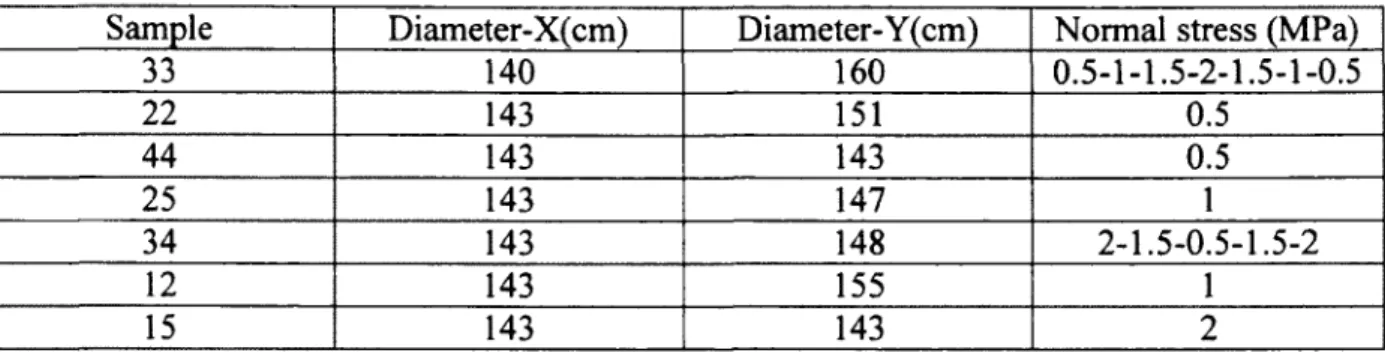
The thesis is divided into 6 chapters. The first chapter includes context, research objectives and originality of the thesis. Chapter II, III, IV and V are presented by published or submitted papers extracted from the results of this study. Chapter II presents a study on characteristic features of acoustic emission parameters during direct shear test of rock joints. In the chapter 3 asperity damage during shear tests of joints is evaluated using acoustic emission. Chapter IV contains the results of AE monitoring during direct shear tests of bonded joints. In Chapter V the results of the AE source localization are correlated with shear damaged zones shown by scanned surfaces and image analysis. Finally Chapter VI provides conclusions and recommendation for future studies. Table 1 -2 to 1 -6 contain characteristics of the artificial and natural joints samples used in this thesis.

Table 1-2: Non-bonded rock-rock joints used in chapter 2 and 5 Sample 33 22 44 25 34 12 15 Diameter-X(cm) 140 143 143 143 143 143 143 Diameter- Y(cm) 160 151 143 147 148 155 143

Normal stress (MPa) 0.5-1-1.5-2-1.5-1-0.5 0.5 0.5 1 2-1.5-0.5-1.5-2 1 2

Table 1-3: Bonded concrete-rock joints used in chapter 3 for study the effect of normal load sample 43-1 43-2 31-1 31-2 54-1 54-2 Diameter-X(cm) 14.3 14.3 14.3 14.3 14.3 14.3 Diameter-Y(cm) 15.5 15.5 15.2 15.2 15.1 15.1 Normal stress 0.25 0.75 0.5 1.25 0.15 0.65

Table 1-4: Bonded concrete-rock joints used in chapter 3 for study the effect of displacement rate sample 32-1 32-2 21-1 21-2 24-1 24-2 Diameter-X(cm) 14.3 14.3 14.3 14.3 14.3 14.3 Diameter-Y(cm) 14.7 14.7 14.7 14.7 14.7 14.7 Displacement rate 0.10 0.15 0.05 0.10 0.20 0.25

Table 1-5: Bonded concrete-rock joints used in chapter 3 for study the effect of bonding percentage sample 42-1 42-2 14-1 14-2 41-1 41-2 Diameter-X(cm) 14.3 14.3 14.3 14.3 14.3 14.3 Diameter-Y(cm) 14.8 14.8 14.8 14.8 15.5 15.5 Bonding (%) 10 28 50 75 0 100 21

Table 1-6: List of natural samples cored from Manic 5 dam and used in chapter 3 Sample number MC4-CC-3.10 MC4-CC-2.34 MC4-CC-10.30 MC6-CC-2.18 MC6-CC-3.97 MC6-CC-8.35 MC4-CC-7.22 MC4-CC-6.98 MC4-CC-9.15 MC6-CC-6.60 MC6-CC-3.45 MC4-RC-13.44 MC6-RC-5.36 MC6-RC-7.63 MC4-RC-5.20 MC6-RC-9.20 MC4-RC-13.76 MC4-RR-5.54 MC4-RR-16.65 MC6-RR-10.48 MC6-RR-6.19 MC6-RR-10.00 MCC8-F-1A MCC8-F-1B MCC8-F-1C Deep (m) 3,10 2,34 10,30 2,18 3,97 8,35 7,22 6,98 9,15 6,60 3,45 13,44 5,36 7,63 5,20 9,20 13,76 5,54 16,65 10,48 6,19 10,00 0,40 0,23 0,50 Diameter (mm) 83 83 83 145 145 145 83 83 83 145 145 83 145 145 83 145 145 83 83 145 145 145 200 200 200 Type Concrete-concrete Concrete-concrete Concrete-concrete Concrete-concrete Concrete-concrete Concrete-concrete Concrete-concrete Concrete-concrete Concrete-concrete Concrete-concrete Concrete-concrete Concrete-rock Concrete-rock Concrete-rock Concrete-rock Concrete-rock Concrete-rock Rock-rock Rock-rock Rock-rock Rock-rock Rock-rock Concrete-concrete Concrete-concrete Concrete-concrete Bonded or non- bonded Non-bonded Non-bonded Non-bonded Non-bonded Non-bonded Non-bonded Bonded Bonded Bonded Bonded Bonded Non-bonded Non-bonded Non-bonded Bonded Bonded Bonded Non-bonded Non-bonded Non-bonded Non-bonded Non-bonded Non-bonded Non-bonded Bonded

2. STUDY ON THE CHARACTERISTIC FEATURES

OF ACOUSTIC EMISSION PARAMETERS

DURING DIRECT SHEAR TEST OF ROCK

JOINTS

Autors and affiliation:

Z. Moradian: PhD student, Universite de Sherbrooke, Faculte de genie, Departement de genie civil.

G. Ballivy: professeur, Universite de Sherbrooke, Faculte de genie, Departement de genie civil.

P. Rivard: professeur, Universite de Sherbrooke, Faculte de genie, Departement de genie civil.

Date of submission: 8 November 2010 Acceptation state: Submitted

Journal: International Journal of Rock Mechanics and Mining Sciences Reference: [IJRMMS-D-10-00324]

Titre francais: Etude des caracteristiques des parametres d'emission acoustique pendant

l'essai de cisaillement direct des joints rocheux

Contribution in paper:

The author ofthe thesis has contributed in this paper as first, principal and corresponding author.

Resume francais:

Afin d'evaluer I'applicabilite de remission acoustique (EA) comme un indicateur de 1'instabilite des discontinuites actives dans les structures d'un barrage, une vaste etude de faisabilite a ete effectuee sur 40 echantillons. A cette fin, des essais de cisaillement direct en charge normale constante (CNC) ont ete realises dans des conditions differentes (avec diverses charges normales et diverses vitesses de deplacement) et differentes caracteristiques (rugosites et pourcentages de liaison). Les signaux d'EA ont ete acquis au moyen de capteurs places sur les echantillons. Une analyse a ete effectuee afin de trouver les differences entre les

parametres d'EA a partir du comportement en cisaillement des joints rocheux pendant les essais de cisaillement direct. L'amplitude, les comptes (counts), l'energie, la duration et le temps de montee, soit les cinq parametres d'EA les plus largement utilises sont compares dans cette etude. Deux methodes ont ete utilisees pour verifier les caracteristiques de ces parametres. Dans la premiere methode, plusieurs echantillons ont ete testes sous des contraintes normales de 0,5, 1 et 2 MPa, respectivement. Dans la seconde methode, la contrainte normale a ete modifiee de 0,5 a 2 MPa dans la section residuelle d'un meme echantillon. Les resultats experimentaux montrent que la charge normale a un effet significatif sur les caracteristiques des parametres d'EA au cours des essais de cisaillement des joints rocheux. Une analyse combinant des parametres d'EA avec le comportement contrainte-deplacement des joints rocheux est utile pour detecter le mouvement de cisaillement et pour determiner les circonstances de la rupture des joints actifs a un stade beaucoup plus precoce, avant une rupture soudaine.

Abstract

In order to evaluate the applicability of the acoustic emission (AE) as an indicator of instability of active joints in dam structures, an extensive feasibility study was done on 40 joint samples. To this end, constant normal load direct shear tests (CNL) were conducted under different conditions (in various normal loads and displacement rates) and different joint characteristics (with various roughness and bonding percentages) and AE signals were acquired using attached sensors to the samples. An analysis was performed in order to find out the differences between acoustic emission parameters in showing shear behavior of rock joints subjected to direct shear test. Amplitude, counts, energy, duration and rise time as the five most widely used AE parameters are compared in this study. Two methods were used to verify the characteristics of these parameters. In the first method several samples were tested under normal stresses of 0.5, 1 and 2 MPa respectively. In the second method normal stress was changed from 0.5 to 2 MPa in the residual section of the same sample. Experimental results showed that normal load has a significant effect on characteristics of AE parameters during shear testing of rock joints. A combining analysis of the AE parameters with stress-displacement behavior of rock joints is useful in detecting shear movement and determining

failure circumstances of active joints at a much earlier stage, before unexpected collapse takes place.

2.1. Introduction

Stability or instability of rock mass mostly depends on rock joints. In order to monitor cracking and damaging of rock mass, instrumentation systems are installed. One of the most precise and fastest methods for monitoring crack initiation and propagation in rock mass is AE. AE is defined as rapid release of elastic waves by cracking and damaging of materials under load. Instability and failure is associated with large number of AE events, so that the greater AE activity the greater is the degree ofthe instability.

Parameter-based and signal-based techniques are two methods for analyzing AE signals which are currently applied. However, where a large number of AE signals have to be analyzed the parameter-based technique is chosen.

The five principal parameters (Figure 2-1) which have been used by researchers and have been accepted through the market processes are 1) amplitude: the highest peak voltage of an AE signal 2) count: number of times that the pulse crosses the threshold 3) duration: time interval between the first and the last threshold crossing 4) energy: area under the envelope of the signal and 5) rise time: time interval between first threshold crossing and signal peak.

Amplitude is directly related to the magnitude of the source event (Pollock 2003, Shiotani 2008). The amplitude is also an important parameter to determine the system's detectability (Shiotani 2008). Count depends on the magnitude ofthe source event (Pollock 2003) and also it depends strongly on the employed threshold and the operating frequency (Shiotani 2008). Duration depends on source magnitude, structural acoustics, and reverberation in much the same way as counts (Pollock 2003). Rise time is governed by wave propagation processes between source and sensor (Pollock 2003). Energy is sensitive to amplitude as well as duration, and it is less dependent on threshold setting and operating frequency (Pollock 2003).

U - Duration (0) - • » ! ! j Counts RiMtknt(R)—»- U — / /

r-^---

T

! If// 1

A

f

Figure 2-1: Common parameters of an AE waveform (Pollock 2003)

Previous researches have addressed application of AE parameters for monitoring rock joints both in laboratory (Li & Nordlund 1990, Hong & Jeon 2004, Rim & Choi 2005) and in site (Sasao et al. 2003 and Shiotani 2006, Ishida et al. 2010).

Li & Nordlund (1990) investigated the characteristics of AE count rate during shearing of rock joints with artificial and natural joints. Rim & Choi (2005) used AE count and energy during constant normal stiffness shear test ofthe artificial saw-tooth joints and replica ofthe natural rock joints. Sasao et al. (2003) used acoustic emission count and interpreted its results during excavation of a rock cliff with opening joints. Shiotani (2006) used AE energy and AE hit (number of detected signals on a channel) rate for evaluation of long-term stability for rock slope by means of acoustic emission technique. Ishida et al. (2010) used AE count rate during an in-situ direct shear test. From all of mentioned researches, it was found that a rapid rise of AE activity is produced as joint is approaching the failure point. Hong and Jeon (2004) showed that the maximum rates of the counts and energy are observed when the stress drops

Although several researchers have used AE parameters during their researches, however there is not a. comprehensive study to show the capability of each parameter in showing shear behavior of rock joints. The principal objective of this study is to find how these parameters detect the initial movement of the joint surfaces, which one has a better indication in showing maximum shear strength, how these parameters change with normal load and finally whether interpretation of these parameters together will give a better insight about failure circumstances of the rock joints. To this end, the characteristics of the AE parameters are investigated by conducting direct shear tests on samples under various constant normal loads.

2.2. Methodology

2.2.1. Samples preparation and properties

Joint samples were prepared by tension splitting of rock cores, with 150 mm diameter, drilled on a large granite block (Barre granite from Vermont, USA). In order to allow the considered shear displacement (maximum 10 mm) without rotation of the upper surface, the shearing area ofthe rock joints was 17660 mm2, greater than 2500 mm2 in ISRM suggested method (Brown

1981). It was tried to prepare sample as close as possible to the natural joints. Table 2-1 shows physical and mechanical properties ofthe rock cores used for this study.

Table 2-1: Physical and mechanical properties ofthe granite rock cores

Parameter Number ofthe tests Average value Bulk specific gravity (-) 3 2.63 P-wave velocity (m/s) 3 4675 Elastic modulus (GPa) 3 58.1 Poisson ratio (-) 3 0.30 Uniaxial compressive strength (MPa) 3 179 27