1
The links between some European financial factors and the BRICS credit
default swap spreads
Kuhanathan ANO SUJITHAN
†Sanvi AVOUYI-DOVI
*First Draft Abstract
Emerging economies and especially the BRICS countries have strong economic ties with the euro area. In addition, the financial crisis in the euro area may have effects on other markets or areas, especially those of the main emerging markets. Credit default swap (CDS) spreads are relevant indicators of credit risks. After identifying a set of fundamental determinants for sovereign CDS spreads, including euro area financial factors and computing Markov switching unit root test, we estimate Markov switching models over the period from January 2002 to August 2012, in order to examine the behaviour of sovereign CDS spreads in the BRICS countries. , i) We detect two different regimes for the BRICS, that finding is backed by conventional robustness checks and economic events; ii) most of the explanatory variables are involved in the determining theses regimes. Thus both financial and real factors have an impact on the relations defining each regime, except for Russia which is only impacted by financial ones. Especially, euro area financial indicators are largely involved in the BRICS sovereign CDS spreads’ dynamics. Besides, the robustness check supports the use of euro area variables as determinants of BRICS sovereign CDS spreads.
JEL classification: C13, G12, G15
Keywords: Credit default swap, BRICS, emerging markets, euro area financial markets indicators, Markov switching
(†) Paris-Dauphine University
(*) Banque de France, Paris-Dauphine University. Corresponding author Tel.: +33142929084, e-mail address: sanvi.avouyi-dovi@banque-france.fr
2
According to the structural model of Merton (1974), the credit spread of a firm should be assessed by its balance sheet asset volatility. Numerous papers tested that hypothesis and tried to show that firm-specific factors can drive the credit spreads of the firm. However, results remain unclear but in broad they support that view. Among others, Das and Tufano (1996) outline the linkage between credit spreads and stock market information. Ericsson and Renault (2000) emphasize that both financial and macroeconomic factors explain credit risk. Collin-Dufresne et al. (2001), Elton et al. (2001), Campbell and Taksler (2003), Huang and Kong (2003) and Ericsson et al. (2008) also contribute to the literature on the determinants of corporate credit spreads. The main finding of these studies is that indicators of liquidity and investors’ risk aversion are key determinants of credit spreads.
Even though sovereign bonds represent one of the most liquid, highly rated and dynamic segment of the market, there are relatively few works devoted to the analysis of dynamics sovereign credit default swaps (CDS). However some studies (among others, Edwards (1986), Berg and Sachs (1988), Duffie et al. (2003), Zhang (2008)) focus on the determinants of sovereign credit spread. By analogy, sovereign credit risk should be influenced by country-specific fundamentals.
Recent empirical papers show otherwise: sovereign credit spreads are strongly linked to global factors and in particular the U.S. ones. For instance, Pan and Singleton (2008) revealed that credit spreads for some emerging countries are strongly related to U.S. stock markets implied volatility. Remolona et al. (2008) tried to solve the “pro-country-specific” versus “pro-global” puzzle. They decomposed CDS spreads into two components: a measure of expected loss (the sovereign credit risk) and a risk premium. The expected loss would be linked to country-specific macroeconomic factors and market liquidity whereas risk premia would be driven by global investors’ risk aversion. In their footstep, Longstaff et al. (2011) used a theoretical model to decompose spreads into expected loss and risk premia. They showed that sovereign risk premia for emerging countries is mainly linked to global factors and particularly to U.S. factors. More precisely, using monthly 5-year senior CDS of 26 countries over the sample from October 2000 to January 2010, Longstaff et al. showed that sovereign risk premia can be explained by U.S. equity, stock market volatility and high yield markets.
More recently, Wang and Moore (2012) investigated the dynamic correlations between 38 emerging and developed countries’ sovereign CDS with the U.S. during the subprime crisis. They showed that since the Lehman Brothers collapse, developed economies especially have had tighter links with the U.S. Fender et al. (2012) found that sovereign CDS spreads changes for emerging countries were mostly related to global and regional factors. The authors used daily CDS spreads for 12 emerging economies from April 2002 to December 2011. They splitted the period into two: one sub-period before the crisis and another after the Lehman Brothers collapse. Using GARCH models, they demonstrated that CDS spread changes stem from U.S. bond, equity, high yield and emerging credit returns, especially in the second sub-period.
Our paper is related to the stand of literature on the pricing and determinants of CDS. It complements and extends the body of works based on those of Longstaff et al. (2011) or Fender et al. (2012). We aim to explore the relation between emerging markets sovereign CDS and the euro area financial and risk factors. This approach seems relevant in the current economic context. In addition, to our knowledge, it has never been explored in the financial empirical or theoretical literature, except Fender et al. (2012) who included ECB interest rates hikes in their model. Indeed, a large body of literature shows that the most significant explanatory variables for CDS spreads are related to the US markets (US stock, and high-yield market returns, volatility risk premium embedded in the VIX index, etc., see, among others, Kamin and von Kleist, 1999, Eichengreen and Moody, 2000, Mauro, Sussman and Yafeh, 2002, Pan and Singleton, 2008, Longstaff et al., 2011, Ang and Longstaff, 2011). Our approach also differs from previous ones as it includes both financial and real factors. Due to the fact that macroeconomic factors are introduced in the model, the empirical analysis is realized with monthly data. This allows us to take into account a set of country-specific fundamentals such as fiscal and trade indicators. We also include the recent financial turmoil period in our sample. Finally, in order to deal with the different phases of the dynamics of CDS spreads, we use a fixed transition probability
3
Markov-Switching Autoregressive Moving-Average (MS-ARMA) model to pinpoint potential regime shifts in the sovereign CDS spreads.
The remainder of the paper is organized as follows. Section I describes the developments of sovereign CDS in the BRICS countries. Section II presents data and descriptive statistics. Section III is devoted to the approach used to investigate the dynamics of sovereign CDS and to the empirical results. Section IV establishes relevance and robustness of the results. Section V concludes.
I. The CDS in the BRICS countries
Credit default swaps (CDS) are financial instruments for hedging and trading credit risk. CDS are insurance contracts offering protection against the default of a debt issuer, corporate or sovereign. Basically, the buyer of a CDS on a certain entity pays to the seller an annuity premium, defined as a percentage on the notional hedged (i.e. the CDS spread). If there is a credit event, which means that the entity fails to meet debt obligation (mainly repudiation, moratorium and restructuring for sovereign entities), it triggers the settlement of the contract. Settlement can be either physical or in cash. In a physical settlement, the buyer sells the bond to the insurance seller at par value. While in a cash settlement, he keeps his asset and receives the incurred losses in cash. The usefulness of CDS is controversial, but they are reliable indicators of risk. In this paper, we analyze five-year dollar-denominated sovereign CDS for the BRICS countries over the period from January 2002 to August 2012. As India never sold debt overseas and CDS are not traded domestically yet, there are no CDS spreads on Indian sovereign debt. India’s sovereign risk is assessed with the cost of protection against a default of State Bank of India (SBI), which is considered as a proxy for the sovereign risk by major markets analysts and data providers such as Credit Market Analysis (CMA) and Reuters.
In 2002, an increasing debt –largely indexed to the US dollar, and a depreciating real rose fears that Brazil might default on its debt following the footsteps of Argentina. Concerns grew when Fitch Ratings lowered the country’s debt rating and Moody’s announced a negative outlook for it. The probable victory of Lula in the upcoming elections was also considered by investors as a source of an uncertainty and a potential threat to the country’s ability to service its debt. Even though, in August 2002 the country benefited from a large loan from the IMF, investors remained concerned. CDS spreads on Brazil reached extremely high levels during the fall, with record levels as high as 3,951 basis points (bps) on October 15th 2002 and only came back down to 2001 levels only in January 2004. During 2004, the spreads rose back to more than 900 bps but not at comparable levels.
From January 2005 to December 2007, the BRICS sovereign CDS spreads remained relatively low. On average 185.5 bps for Brazil, still recovering from the 2002 episode, 71.9 bps for Russia, 69.2 bps for India, 20.7 for China and 50.6 bps for South Africa. In 2008, CDS spreads started rising for the BRICS, probably as a consequence of the global financial crisis. Indeed, after, the collapse of Lehman Brother, all spreads increased sharply (September and October, see Appendix 2) as investors expected governments to be involved in bank bailouts plans that would rise tremendously their spending. The increase was particularly marked for State Bank of India’s CDS spread, due to the nature of its activity and its participation in the global banking network. However, SBI CDS spreads remained much lower than those of large Indian private banks1.
The other country for which CDS spread experienced a very sharp rise in the last quarter of 2008 is Russia. That rise was due not only to the large banks bailout plan announced by the government but also to other factors. In October, Russia had large capital outflows as investors withdrew their money
1
For example, in October 2008 the CDS for 5 year-maturity senior debt issued by ICICI Bank, one the Indian largest private bank, were trading 1,000 bps higher than SBI CDS.
4
for the country. The stock market felt sharply (over 60% in a few weeks). Coupled with fall in oil prices that threatened government revenues and the country’s growth, investors grew concerned about the creditworthiness of the Russian government. All of the above led Moody’s to downgrade Russia’s outlook from “stable” to “negative” and Standard & Poor’s to issue a warning.
In the second half of 2010, at the beginning of the euro area sovereign-debt crisis, BRICS CDS spread rose but remained relatively low compared with the levels observed in the aftermath of Lehman Brother’s collapse. Since the second half of 2011, spreads have started to rise again. The rise in spreads resulted from that of uncertainty regarding growth prospects in the BRICS countries as the crisis deepened in Europe and BRICS governments were expected to go on large spending sprees. These concerns were especially high regarding Russia and India. Indeed, Russia has strong economic links with Western Europe whose economic slowdown could endanger Russian economy. India has been struggling with rising inflation and a slowing pace of growth which can lead to a loosened fiscal policy. Those factors led Standard & Poor’s to issue a downgrade warning in June 2012 and Fitch Ratings to downgrade the country’s outlook to “negative”. All the above mentioned explains why the SBI CDS spreads remained above the other BRICS countries’ spreads in the second half of 2012.
II. Data and descriptive statistics
II.1. Test for stationary in the framework of a Markov-Switching model
In the conventional ADF test, the presence of a unit root is based on the following regression:
∆𝑦
𝑡=
𝜇 + 𝜑𝑦
𝑡−1+ ∑
𝑗=1,…,𝑘𝜑
𝑗∆𝑦
𝑡−𝑗+ 𝜐
𝑡 under the null hypothesis, φ = 0;𝜐
𝑡 is a zero-mean whitenoise. According to these tests, we can accept the hypothesis that the variables under review are I (1) (see Appendix 4), As a consequence, we focus in the following on their log variations from one month to the other which are stationary.
For the Markov-switching unit root test, we perform the Markov-Switching Augmented Dickey–Fuller (MS-ADF) test proposed by Hall et al. (1999) 2 in order to detect explosive bubble behaviors in the variables dynamics.
Given the MS-ADF model specified as
Δ𝑦𝑡 = 𝜇𝑆𝑡+ 𝜙𝑆𝑡𝑦𝑡−1+ � 𝜓𝑆𝑡,𝑖Δ𝑦𝑡−𝑖+
𝑘
𝑖=1
𝜎𝑆𝑡𝜀𝑡,
where, 𝜙𝑆𝑡= 𝜙1+ (𝑆𝑡− 1)(𝜙2− 𝜙1) is the ADF coefficient. If we refer to the regime with a larger (resp. lower) ADF coefficient as regime 1 (resp. 0), the MS-ADF bubble test is defined as follows:
- In regime 2, the unit root null hypothesis is 𝜅1≡ max(𝜙1, 𝜙2) = 0 against the explosive alternative 𝜅2 > 0.
2
Although this test was designed for Markov-switching models with fixed transition probabilities (FTP), we use it in our time-varying transition probabilities (TVTP) framework, since no adapted tests exists in the literature in such a framework. Additional study on the unit-root tests for MS-TVTP models would be an interesting research topic.
Also, lets note that first differences of our variables or of the logarithm of the variables are stationary series under standard unit root tests (see Appendix 2).
5
- In regime 1, the unit root null hypothesis is 𝜅0≡ 𝑚𝑖𝑛(𝜙1, 𝜙2) = 0 against the stationary alternative 𝜅1< 0.
Following van Norden and Vigfusson (1998) and Shi (2012), we run parametric bootstrapping to obtain the critical values of the MSADF test. 1000 replications are used in the bootstrapping, with the estimated coefficients of the model as priors.
We reject the unit root null hypothesis of 𝜅2 for Brazil and South Africa series at 1% significance levels and for India and Russia at 5% significance level. We fail to reject that for China at 10% confidence level (see Table 1). Furthermore, we fail to reject the unit root null hypothesis in regime 1 of all series at the 10% significance level. In other words, series for Brazil, South Africa, Indian and Russia are mixtures of a unit root process and an explosive process, whereas Chinese CDS seem to be only driven by random walk processes.
6 Table 1 – MS-ADF tests
Estimates Critical Values
Coefficients ADF Stats 10% 5% 1%
CDS Brazil 𝜅1 -0.05 -31.30 -41.59 -43.55 -49.30 𝜅2 0.02 1.67 1.41 1.51 1.57 CDS China 𝜅1 -0.15 -1.97 -9.19 -10.04 -11.26 𝜅2 0.67 0.74 2.45 2.52 2.58 CDS India 𝜅1 -0.19 -2.05 -15.52 -17.10 -19.71 𝜅2 0.96 0.06 -0.04 0.04 0.09 CDS Russia 𝜅1 -0.45 -0.04 -15.70 -16.11 -17.25 𝜅2 0.22 1.12 0.89 1.04 1.17 CDS South Africa 𝜅1 -0.13 -1.25 -7.75 -8.90 -19.78 𝜅2 0.78 0.24 -4.81 -0.95 0.08
Source : authors’ calculations
As a consequence, the univariate Markov-switching approach seems relevant for studying dynamics of BRICS CDS. Even though, it is less clear with the series for China, we will include it in further analysis. II.2 Endogenous variables
The CDS spreads data are extracted from the Bloomberg database. Bloomberg collects market data from various industry sources. We use dollar-denominated 5-year contracts on senior international debt, which are the most liquid and active segment of the market. The sample goes from January 2002 to August 2012 for Brazil, South Africa and Russia and from February 2003 to August 2012 for China goes. As mentioned above, there are not CDS spreads on Indian sovereign debt. We use CDS spreads on State Bank of India (SBI) as a proxy of Indian sovereign spreads. This variable goes from January 2005 through December 2009 in the Bloomberg database and from October 2008 to August 2012 on the Thomson-Reuters database. In order to build a homogenous and coherent sample from January 2005 to September 2012, we perform a calculation based on a simple regression on the overlapping sample. The coefficients of this regression enable us to generate the missing values in order to complete the time series of Thomson-Reuters. Due to the results of the tests for stationary, only the first-order differences of the variables (or those of the log of variables) are used in the empirical analysis.
Means of first-order difference of the CDS spreads range from -0.015 for Brazil to 0.018 for India (see Appendix 4). All series are relatively volatile with standard deviations more than ten times their averages (0.20). We accept the presence of fat tails and the hypothesis of symmetry. As a consequence, the CDS spreads are not normally distributed.
II.3 Explanatory variables
First, we use a set of country-specific financial factors as the CDS explanatory variables. Most indices are drawn from the Bloomberg database. We use the Shanghai Composite Index for China, the IBOVESPA for Brazil, the Sensex Index for India, MSCI Russia and MSCI South Africa. Every first-order difference of the log of the index shows asymmetry (negative skewness) and leptokurtic distribution. We calculated also monthly first-order difference for each country’s exchange rate against the euro. Exchange rates are also extracted from the Bloomberg database. These time series display the
7
same features except for the euro-rupee and the euro-yuan exchange rates that do not reveal any asymmetry.
Second, we incorporate a set of country-specific non-financial factors in relationship with debt and external links. Hence, we computed monthly changes in trade-balance-to-GDP ratio, and monthly changes in the foreign-currency-reserves-to-GDP ratio. These time series are provided by the International Monetary Fund and extracted from the Datastream. And we also introduce monthly changes in government-finance-balance-to-GDP ratio. Figures are provided by national sources.3 Third, we take into account financial indicators from the euro area, such as the monthly returns of the Dow Jones Eurostoxx 50 (SX5E). The log-return series has the same features as those mentioned above. We include the first-order difference of the log of VStoxx index which indicates the implied volatility for the SX5E. This indicator acts as a measure of investors’ risk aversion for euro area assets. The series displays a leptokurtic but symmetric distribution. Finally, include the first-order difference of the Thomson-Reuters Eurozone Corporate Benchmark 5 year Yield for AAA issuers. All series indicates asymmetry and with the exception of the corporate yield, they all show leptokurtic distributions.
In order to simply test the existence of a link between BRICS sovereign risk that of the Euro area countries, we computed correlations between series of various CDS spreads (taken in first-order difference of the log,see Appendix 3). Correlation between BRICS CDS spreads and Euro area CDS spreads is on average 21.3%, which is rather low. Correlation between France sovereign CDS and Brazil sovereign CDS is relatively high (32.9%); whereas correlation between Spain and India is the lowest (9.3%). As a consequence, we do not include Euro area CDS spreads has explanatory variables of BRICS sovereign risk dynamics.
As expected, correlation is much higher within the BRICS. This result could be the basis of an alternative approach of the BRICS CDS Dynamics.
Finally, due to the key role played by the commodities prices in BRICS (see above), we take into account commodity prices in our analysis by using the first-order difference of the log of the Commodity Research Bureau (CRB CMDT) Index, which is a benchmark for 22 basic commodities.
III. Model specification
Business cycle research has revived interest in the co-movement of time series which can move between states/regimes of high and low growth, for instance. The general idea of this approach is that the dynamics of some variables depend on a latent non-observable variable
𝑠
𝑡 (if we assume that there are k states, then𝑠
𝑡= 1, … , 𝑘)
which represents different states of economic activity. It is often convenient to adopt the two-state version of Hamilton's (1989) Markov-switching model (𝑠
𝑡= 1, 2
), which is a useful approach for the detection and dating the business cycle turning points.III.1. Markov-Switching Autogressive Moving-Average model (MS-ARMA)
Markov-Switching Autoregressive Moving-Average (MS(k)-ARMA(p,q)) models is considered as extensions of the well-known ARMA(p,q) model that allow ARMA(p,q) coefficients to be
3
As GDP figures are available only in quarterly frequency, for all data involving GDP ratio we perform quarterly calculations. Then we computed monthly ratios by assuming that intermediate monthly points were on a natural cubic spline.
8
dependent. One of the main advantages of MS models is that it introduces the non-linearity and asymmetry in the time series dynamics.
Let’s consider the most general form of the univariate MS (k)-ARMA(p,q) model:
𝑦
𝑡= 𝑐
𝑆𝑡+ ∑
𝜙
𝑆𝑡𝑦
𝑡−𝑖𝑝
𝑖=1
+ 𝜀
𝑆𝑡𝑡+ ∑
𝜓
𝑆𝑡𝜀
𝑆𝑡−𝑗𝑡−𝑗 𝑞𝑗=1 (1)
Each of the k regimes is associated with a single conditional distribution of the endogenous variable yt, where the intercept
𝑐
𝑆𝑡 is related to the state that prevails; the coefficients of the AR (p) process,𝜙
𝑆𝑡, and those of the MA(q) process,𝜓
𝑆𝑡, are also state-dependent (they depend on the state𝑆
𝑡). In
addition, the variance of𝜀
𝑆𝑡𝑡 changes with the states, in other words, the homoscedasticity hypothesis is rejected.𝜀
𝑡~𝑁(0, ∑
𝑆𝑡)
(2)∑
𝑆𝑡= �
𝜎
1,12⋯ 𝜎
𝑘,12⋮
⋱
⋮
𝜎
1,𝑘2… 𝜎
𝑘,𝑘2�
(3)For the sake of simplify, the previous matrix is assumed to be diagonal in the empirical applications. The state variable St is assumed to follow a first order Markov-process, which means that the current state only depends on the previous one.
Pr (𝑆
𝑡= 𝑗�𝑆
𝑡−1= 𝑖) = 𝑝
𝑖𝑗 (4)where
𝑝
𝑖𝑗 is the probability that state i will be followed by state j. Due to the hypothesis that𝑝
𝑖𝑗 is not time varying, our model is a fixed transition probability Markov-Switching Autoregressive Moving-Average(MS-ARMA) model.4
We can define the transition matrix, P (k x k), as follows:
𝑃 = �
𝑝
11⋮
⋯ 𝑝
⋱
𝑘1⋮
𝑝
1𝑘… 𝑝
𝑘𝑘�
(5)With
∑
𝑘𝑗=1𝑝
𝑖𝑗= 1
where i=1, …, k and0 ≤ 𝑝
𝑖𝑗≤ 1
Now, we are going to analyze a MS(k)-ARMA(p,q) for each country, the empirical analysis focus on
two states (St = 1, 2) model.
4
According to Filardo (1994), the transition probabilities can vary across time. Empirically, the evolution of the unobserved state will depend on available information represented in the time series zt. The time-varying
transition probabilities (TVTP) matrix is:
Pr�𝑆𝑡= 𝑠𝑡|𝑆𝑡−1= 𝑠𝑡−1,𝑧𝑡� = � 𝑞(𝑧1 − 𝑞(𝑧𝑡) 1 − 𝑝(𝑧𝑡)
𝑡) 𝑝(𝑧𝑡) �,
9
It is worth noting that McConnell and Perez-Quiros (2000) proposed an augmented version of standard Markov-Switching model in two ways: i) the dynamics of the mean and the variance are driven by two separate states; ii) the state process for the mean depends on the state of variance. If we specify two processes for mean and variance dynamics, due to the small size of the data sample, we cannot guarantee the accuracy, the robustness of our estimation. As a consequence, we do not follow McConnell and Perez-Quiros proposals and we impose a single latent unobservable variable for the description of the states of mean and variance dynamics. However, our model is governed by a state dependent variance Markov-switching process.
Maximum likelihood estimation of the model can be based on a version of the Expectation-Maximization (EM) algorithm discussed in Hamilton (1990).5 By inferring the probabilities of the unobserved regimes conditional on an available information set, it is possible to reconstruct the regimes. Here the model is estimated with maximization process which is implemented using the Broyden-Fletcher-Goldfarb-Shanno (BFGS) method.
As
𝑓(𝑦
𝑡|𝑆
𝑡= 𝑗, Θ)
is the likelihood function for regime j conditional on a set of parameters Θ, assuming that there is two-sate model, k=2, our log likelihood is given by:ln 𝐿 = ∑
𝑇𝑙𝑛
𝑡=1
∑ [𝑓(𝑦
2𝑗=1 𝑡|𝑆
𝑡= 𝑗, Θ)Pr (𝑆
𝑡= 𝑗)]
(6)III.2. Empirical results
First, we run ARMA-type regressions for which we notice: i) only a few variables are significant effects on CDS spread changes (see Appendix 6); ii), with AR recursive models, we observe that coefficients vary over time, supporting an approach of Markov Switching modeling (Appendix 7). We did not get a truly consensual model for the BRICS countries (in terms of lag in the MS-ARMA) via the conventional model selection criteria (AIC, SIC, etc.). However, the MS (2)-ARMA (1,1) model (see Appendix 8) seems convenient for the five markets under review. As a consequence, for each country, we estimate the following model:
𝑦
𝑡= 𝑐
𝑆𝑡+ 𝜙
𝑆𝑡𝑦
𝑡−1+ 𝛼
𝑆𝑡1𝑥
1,𝑡−1+ ⋯ + 𝛼
𝑆𝑡𝑘𝑥
𝑘,𝑡−1+ 𝜀
𝑡+ 𝜓
𝑆𝑡𝜀
𝑡−1 (8) Where𝑥
1, 𝑥
2, … , 𝑥
𝑘 is the set of explanatory variableswith:
𝜀
𝑡~𝑁(0, 𝜎
𝑆2𝑡)
(9)𝑆
𝑡= 1, 2
(10)For all countries, the model detects two different states, one that we qualify as “low growth” regime during which average first-order difference of log of CDS spreads is low (respectively -3.7%, -1.3%, -5%, -3.2% and -3.7% for Brazil, China, India, Russia and South Africa, Tables 1a to 1e); the second one is called “high growth” regime, it is associated with higher average first-order difference of log of
5
See Diebold et al. (1994) for some details on the EM algorithm applied to the regime switching model with time-varying transition probabilities.
10
CDS spreads (7.6%, 10%, 3.4%, 6.5% and 1% for respectively Brazil, China, India, Russia and South Africa). AR terms and intercepts are significant in both states everywhere, MA terms are also significant except in high growth regime for China, India and Russia.
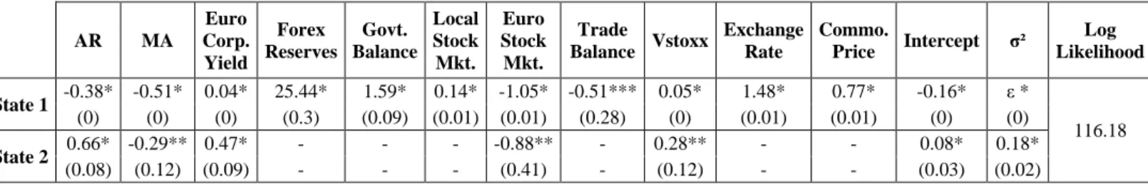
Regarding the “low growth” regime, non-financial factors do not have significant impact on the CDS except in South Africa where the parameters of these factors are all significant. For India, trade balance and government balance have a significant impact; in the case of Brazil, the coefficient of foreign currency reserves is a significant. Commodities prices also have an impact on CDS spreads. Regarding financial factors, except for Russia, the domestic stock market, the exchange rate, the Dow Jones Eurostoxx 50 and the VStoxx impact the CDS spreads. Besides, the euro corporate yield parameter is significant everywhere.
The dynamics of CDS are quite different in the high growth regime. While looking at the equation for Russia, we note that apart from AR term and the intercept, the financial factors, except the exchange rate, have significant parameters. South African CDS spreads are influenced only by euro factors parameters (the euro corporate yield, the Dow Jones Eurostoxx 50 and the VStoxx) and ARMA terms. Here, the coefficients are of the opposite sign or much higher. In the case of Brazil the parameters (except foreign currency reserves) are significant, and the figures for the coefficients already present in the former state are very different. All parameters are significant for India. The coefficients of determinants of China’s CDS spread (with the exception of the MA term, the government balance and the exchange rate) are significantly different from 0.
According to the results of the estimation, the euro area factors are involved in the determination of BRICS CDS spreads dynamics in both regimes.
. Besides (Table 1f), the duration of “low growth” is higher than that of regime of “high growth” except for the South Africa and India. Indeed except for the South Africa, the duration associated with “low growth” regime is between 3.5 months (Russia) and 13.7 months (China). By contrast, the duration corresponding to regime of high-growth shows a minimum of 1.5month (Russia) and a maximum of 2 months (China). For instance, regarding Brazil, the duration of “low growth” regime is 4.74 months versus 1.94 month for “high growth” regime. South Africa and India are the only place where the durations in regime of high-growth are significantly greater than those of “low growth” regime (4.67 months versus 1.35 months for South Africa, 3.5 months versus 1.47 months for India). Focus on the period corresponding to the euro zone sovereign crisis
We can acknowledge that the euro debt current crisis started in the last quarter of year 2009, while concerns regarding Greece emerged and the cost of borrowing started rising for the country. Looking at the last 36 months, we count the number of months that are classified in the “high growth” state: for China that figure is as low as 2; in the case of Brazil, 12 months are classified as such and 8 months for Russia. That figure goes as high as 27 months for India and 29 months for South Africa.
In addition, there is no simultaneity in the regimes across countries (Figure 1). There are 38 periods when at least 3 countries are in the “high growth” state and only 7 months when all countries are simultaneously in that state. Even though there are only a few periods where we observe simultaneity, it is interesting to note that it occurs during major global events: the subprime crisis and the growing concerns on its impact on global economy (mid 2007 and during the first half of 2008), the Lehman collapse (September and October 2008); and when long-term interest rates started to diverge in the euro area (August and September 2011).
11
We displayed previous studies’ results (Longstaff et al. 2011, Fender et al. 2012, Table 2) in terms of significant coefficients. Some of the results presented here are complied with the findings of Longstaff et al. or Fender et al. However another part of results is challenging their analysis6.
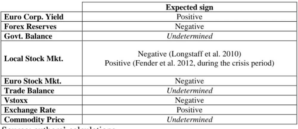
Besides from China in the “low growth” regime, for all countries, the euro corporate high yield’s coefficient is positive and the sign of this coefficient is economically intuitive and consistent. Contrarily to results from previous studies, all countries show a positive coefficient for foreign currency reserves changes. Previous studies did not consider government budget balance; broadly we find a positive effect of this factor (except for India in the case of the “high growth regime”). When it comes to local stock market, there is no consensus within the literature: in Longstaff et al. (2011), the coefficient is negative whereas the coefficient is significant only during the crisis period and positive in Fender et al. (2012). Our results are in line with the findings of Fender et al, the coefficients are positive for most countries, except for Brazil in the “low growth” regime and China in the “high growth” regime where it is negative.
The impact of DJ Eurostoxx 50 is negative in the high growth regime for Brazil, China and Russia, and during the both regimes for India and South Africa; which is consistent with the literature. We also find that such coefficient is positive in the “low growth” regime for Brazil, China and Russia. The coefficient of trade balance is positive in the “high growth” regime for Brazil and China. For South Africa, the coefficient is negative in the “low growth” regime. In the case of India, it is negative in both regimes. In general, volatility premium negatively influences the CDS spread in the literature. Our findings are rather challenging as there is no homogeneity, neither in sign nor among countries: for Brazil and South Africa coefficients are positive in both regimes. China shows a positive coefficient in the “low growth” regime and a negative one in the “high growth” regime while India is in the opposite configuration. Russia’s CDS spread is impacted negatively in the “high growth” regime. Our results regarding exchange rate impact are broadly consistent with the former studies: coefficients are mostly positive with exception of Brazil which show negative coefficient in the “high growth” regime. Finally, as we analyze the commodity factor, absent in the literature, coefficients are mainly positive except for India and Brazil (negative in the “high growth” state).
Table 2a – Brazil MS-ARMA(1,1)
AR MA Euro Corp. Yield Forex Reserves Govt. Balance Local Stock Mkt. Euro Stock Mkt. Trade Balance Vstoxx Exchange Rate Commo. Price Intercept σ² Log Likelihood State 1 0.72* -0.42* 0.15* 5.82* - -0.8* 0.77* - 0.4* 0.8* 0.98* -0.13* 0.16* 74.68 (0.04) (0.05) (0.03) (0.49) - (0.12) (0.2) - (0.07) (0.16) (0.28) (0.01) (0.01) State 2 -0.73* -0.24* 0.72* - 2.5* 1.46* -2.9* 22.01* 0.12* -2.28* -0.28* 0.19* 0.01* (0.03) (0.03) (0.02) - (0.09) (0.09) (0.1) (0.67) (0.02) (0.09) (0.08) (0) (0)
6 For instance, the coefficient of the lagged value of the endogenous variable is not always positive: i) in the case of India, the coefficient is negative, regardless of regimes; for Russia and South Africa, they are negative in the “low growth” regime while positive in the “high growth” regime, Brazil is in the opposite situation and results for China are in line with previous studies.
12 Table 1b – China MS-ARMA(1,1)
AR MA Euro Corp. Yield Forex Reserves Govt. Balance Local Stock Mkt. Euro Stock Mkt. Trade Balance Vstoxx Exchange Rate Commo. Price Intercept σ² Log Likelihood State 1 0.45* -0.44* -0.13*** - - 0.56* 1.03** - 0.25** 1.2* 1.44* -0.05** 0.11* 52.56 (0.12) (0.14) (0.07) - - (0.17) (0.47) - (0.1) (0.41) (0.46) (0.02) (0.01) State 2 1.07* - 0.96* 0.03* - -0.85*** -4.04* 28.04** -0.4** - 3.9** 0.29* 0.12* (0.12) - (0.15) (0.01) - (0.48) (1.09) (10.63) (0.18) - (1.74) (0.05) (0.03)
Table 1c – India MS-ARMA(1,1)
AR MA Euro Corp. Yield Forex Reserves Govt. Balance Local Stock Mkt. Euro Stock Mkt. Trade Balance Vstoxx Exchange Rate Commo. Price Intercept σ² Log Likelihood State 1 -0.33* 0.08* 0.26* ε* 0.49* 0.56* -2.05* -3.3* -0.49* 1.12* 1.66* -0.17* ε * 112.13 (0.01) (0) (0) (0) (0.01) (0.01) (0.01) (0.02) (0) (0.01) (0.01) (0) (0) State 2 -0.2* - 0.64* ε * -0.09* - -1.11* -8.78* 0.03** 0.29* -1.19* 0.03* 0.19* (0.01) - (0.02) (0) (0.03) - (0.04) (0.37) (0.01) (0.06) (0.03) (0) (0.02)
Table 1d – Russia MS-ARMA(1,1)
AR MA Euro Corp. Yield Forex Reserves Govt. Balance Local Stock Mkt. Euro Stock Mkt. Trade Balance Vstoxx Exchange Rate Commo. Price Intercept σ² Log Likelihood State 1 -0.43* -0.3* 0.2** - ε * - - ε *** - - 1.56* -0.08* 0.08* 65.43 (0.13) (0.09) (0.08) - (0) - - (0) - - (0.44) (0.01) (0.01) State 2 0.92* - 0.33* ε ** ε ** 0.83* -3.84* - -0.22*** - - 0.14* 0.12* (0.1) - (0.1) (0) (0) (0.2) (0.56) - (0.12) - - (0.02) (0.02)
Table 1e – South Africa MS-ARMA(1,1)
AR MA Euro Corp. Yield Forex Reserves Govt. Balance Local Stock Mkt. Euro Stock Mkt. Trade Balance Vstoxx Exchange Rate Commo. Price Intercept σ² Log Likelihood State 1 -0.38* -0.51* 0.04* 25.44* 1.59* 0.14* -1.05* -0.51*** 0.05* 1.48* 0.77* -0.16* ε * 116.18 (0) (0) (0) (0.3) (0.09) (0.01) (0.01) (0.28) (0) (0.01) (0.01) (0) (0) State 2 0.66* -0.29** 0.47* - - - -0.88** - 0.28** - - 0.08* 0.18* (0.08) (0.12) (0.09) - - - (0.41) - (0.12) - - (0.03) (0.02)
Standard errors are in parenthesis. *,**,*** denotes respectively 1%, 5% and 10% significance Table 1f – Durations (months)
Brazil China India Russia South Africa
Low growth
Regime 4.74 13.71 1.47 3.52 1.35
High growth
Regime 1.94 2 3.5 1.54 4.67
13 Table 3 – Expected effects
Expected sign
Euro Corp. Yield Positive
Forex Reserves Negative
Govt. Balance Undetermined
Local Stock Mkt. Negative (Longstaff et al. 2010)
Positive (Fender et al. 2012, during the crisis period)
Euro Stock Mkt. Negative
Trade Balance Undetermined
Vstoxx Negative
Exchange Rate Positive
Commodity Price Undetermined
Source: authors’ calculations
Figure 1 – Number of countries in high growth regime
IV. Economic relevance and robustness check
IV.1. Regimes shift and stylized facts
In this section, we proceed to a country-level analysis in order to identify domestic events that could explain the regime shifts. We looked for events and announcement that were conveyed to the public and to investors using the Bloomberg news database and Factiva. We will not mention repeatedly the impacts of the subprime crisis, the Lehman collapse or the euro debt crisis.
Regarding Brazil, during mid-2002, the model detects several shifts to high growth regime. Such a phenomenon can be explained by both domestic (Market fears that Lula that could win the presidential race), regional (Brazil could follow the footsteps of Argentina and default on its debt) and global factors (“Enron effect”). In 2005, the U.S. Fed raised interest rates for more than ten consecutive times and U.S. economic data prompted some concerns the pace of increases could become even more
0 1 2 3 4 5
6 Subprime crisis and
Lehman collapse
Euro debt crisis
14
aggressive. Hence, emerging sovereign debt spreads rallied. Moreover in Brazil, the Lula administration was hit by a corruption scandal which was widely considered by investors as the worst crisis yet faced by the Brazilian President. We can observe however that CDS levels were nothing comparable with those of 2002-2003. Rises in CDS spreads during mid-2006, which were detected by our model, stem essentially from U.S. factors and uncertainty around U.S. monetary policy. The shifts during the second half of 2007 were mostly fallouts of the U.S. subprime crisis; we do not observe any significant domestic or regional event affecting the cost of protection against a Brazilian default. During 2008, CDS spreads for Brazil relatively increased; investors were expecting the global economic turmoil to have a negative impact on the Brazilian economy. Negative global economic outlook along with an announcement made in April 2009 in which the government revealed a lower fiscal surplus target led put pressure on Brazilian CDS. Late 2011, investors were concerned that even though Rousseff’s government has improved the fiscal accounts in 2011, there would be increased pressure to loosen fiscal policy and the government is very likely to succumb to such pressure. The expected economic downturn and measures such as the upcoming rise of 14% in minimum wage prompted investors to believe that revenue would be weaker.
For China, despite an upgrade in its sovereign rating in the first half of 2007, CDS for China rose during through the second half of the year (here signaled by an “high growth” regime) until June 2009 because of rising concerns that the impact of the subprime crisis could be greater on China than expected. In addition, the central government implemented a four trillion Yuan (around 590 billion US dollars) stimulus package in late 2008, that plan did not immediately restore investors’ confidence. Hence, we note a persistence of high growth state despite the stimulus package. Indeed, the positive effects of such a package remained uncertain until mid-2009. In June 2009, the World Bank raised its growth forecast in the country for 2009 from 6.5% to 7.2%. After that we observe that CDS spreads changes are lower and the model is back in the low growth regime. In the end of the third quarter of 2011, Chinese CDS spreads are again in a high growth regime obviously because of the euro area situation.
Regarding India, our model finds that the country is in a “high growth” regime several times from March 2005 to June 2006 due to several country specific factors: India’s balance of payments has been hit by the high prices of recent past months; Congress-led government approved a budget with significant new spending programs for the poor and reconstructions following the tsunami of December 2004. From 2007 to 2008, India has been in the “high growth” regime 18 times out of 24. This was due to global factors (subprime crisis, Lehman collapse) but also to fears regarding India’s economy: a monetary policy that was judged too loose, growing inflation, a regulatory framework that is not liberalized as required by global investors (especially regarding FDI). The unveiling of a four billion US dollars fiscal stimulus package in early December 2008 and the announcement of a second round of the fiscal stimulus package in January 2009 seems to have had a positive effect on India’s sovereign risk. We observe regime shifts from high growth to low growth in February 2009. The next “high growth” state is detected in June 2009. From mid-2009 to mid-2012, Indian CDS spreads have been in “high growth” regime 30 months out of 36. We can attribute this phenomenon to global factors but also to domestic factors: growing inflation, decreasing domestic consumption and volatile fiscal policy. Eventually, the policy makers stated that monetary policy would not be loosened and the government also injected funds into the public banking system (1.6 billion U.S. dollars for SBI) which smoothened up confidence on India and its financial structure. Then, the high growth regime disappeared after June 2012.
In 2002, we observe four “high growth” regimes in Russian CDS spreads: this is mainly due to growing domestic inflation and to global financial unrest as other emerging economies such as
15
Argentina or Brazil’s sovereign risk was rising. From 2004 to 2006 the model detects regime shifts which are simultaneous to domestic events/concerns: political uncertainty (following the terrorist attack on Moscow underground train, President Putin sacked the government; there was a doubt about the ability and willingness to pursue economic reforms by the new government); inflation is a growing concern, the banking system is surrounded by uncertainty, political interference in corporate matters, a strengthening rubble. During the period from 2007 to 2009, there were several episodes of “high growth” regime, these stem essentially from various reasons: deteriorating relations with the West, spreading global crisis, decreasing oil price, financial unrest (chaos gained the stock markets which had to freeze trading on October 7th), and negative economic outlook. Since 2010, there are only 8 months classified as “high growth”, and these shifts can be explained by punctual stress (the severe heat wave that led Russia to adopt protectionary, the banking system still experienced episodes of stress, Putin’s victory in the presidential race; Putin promised increased state wages, pensions and welfare payments.)
The model reveals too many regime shifts for South Africa (98 periods in total!), it is difficult to list all events that might explain CDS spreads changes and regime shifts. Even though, we list some of the main events regarding South Africa:
- 2002-2003: Pressure from rising currency, risks of a comeback of inflation, anticipated elections programmed for 2004
- 2004-2005: High metal prices and capital flows boost foreign currency reserves, inflation is contained but output remains low. Deputy President is sacked after a corruption case in June 2005. Huge strike in the gold mining industry takes place in August 2005.
- 2006-2007: Low inflows of capital and especially FDI inflows raise concerns (negative in 2006). Inflation becomes quite high in 2007 and current account keeps deteriorating. In June 2007, there is a major strike of public-sector workers. - 2008-2009: Trade suffers from global turmoil. Power crisis reveals infrastructure and investments’ weakness. Unemployment is increasing steadily. Credit crunch is affecting the economy. Trade liberalization could be stopped and barriers erected. Social unrest may lead to populism and loose fiscal policy.
- Since 2010: South Africa hosted the Football World Cup in 2010. Inflation has fallen sharply but output is not growing as rapidly as expected in 2010. Unemployment is still alarmingly high and social divisions are rising paving the way to a more left-wing policy. In May 2011, a new company act came into force and will be broadly positive for business in South Africa. In 2012, one of the major concerns for business and investors is the rising cost of labor.
IV.2. Robustness check in terms of specification
To examine the robustness of our model, we compare it with the benchmark linear non switching ARMA model (Table 3). Then, we estimate a less flexible MS(2)-ARMA (1,1) in which the variance is not state dependent (
𝜎
1= 𝜎
2)
(see Appendix 10). For the sake of stability analysis, we run a MS(2)-ARMA(1,1) model in which the variance is state-dependent over the period January 2002 – August 2008, prior Lehman Brothers collapse (see Appendix 11). Finally, we estimate MS(2)-ARMA(1,1) models including U.S. variables (see Appendix 12 and 13).16
Before comparing the results of the estimations of the previous models, we test the hypothesis of linearity. However, it is not simple to perform a formal and powerful test of the Markov-switching model against linear alternatives. Indeed, under the null hypothesis of a single regime, due to the presence of nuisance parameters, the conventional likelihood ratio tests are not asymptotically χ2 -distributed.
Recent large body of econometric literature is devoted to the identification and the tabulation of theoretical distributions under the null hypothesis (Garcia, 1998; Cho and White, 2007; Carter and Steigerwald, 2012). To our knowledge, the current results regarding the asymptotical distributions under the null hypothesis only apply to the specific cases. More precisely, these distributions depend among others on the set of parameters of the model under review.
One way to reach an acceptable result is to use the linearity tests of Davies (1987) with the approximations to the critical values. These tests could be completed by alternative tests such as the regime classification measure (RCM) suggested by Ang and Bekaert (2002).
The decision’s rule could be: a good Markov-switching model should reflect the null hypothesis of a single-regime (linearity hypothesis) and has a RCM statistic below 50. The results show that the MS-ARMA model with state-dependent variance dominates the others for the BRICS, except in Russia where the MS-ARMA model without the state-dependent variance prevails. The LR ratios tests broadly confirm the previous results. These results validate the relevance of the hypothesis of the presence of two regimes.
In addition, the estimation of the MS-ARMA model with state-dependent variance over the period January 2002-August 2008 confirm the existence of two regimes for the BRICS (see Appendix 11); broadly, LR tests and RCM statistics confirm the superiority of our set of models (except for Russia – lower RCM and higher LR ratio; and India – lower RCM).
Comparison with models including U.S. variables
In order to test the relevance of introducing the Euro area variables, we estimate the models with U.S. variables. First we replace Euro area variables by U.S. variables in our models. Then, we introduce both Euro area and U.S. variables in our regressions in order to see the outstanding parameters. As a consequence, we take into account: i) the monthly returns of the Standard & Poor’s 500 index; ii) the first-order difference of the log of the Standard & Poor’s implied volatility index (the VIX index); iii) exchange rates versus the U.S. dollar iv) Thomson-Reuters U.S. Corporate Benchmark 5-year Yield for AAA issuers. The latter time series started in April 2004, we did a simple retropolation using Bloomberg data for the same maturity and type of issuer in order to evaluate the missing values of this yield.
First, we scrutinize the results of the models only including U.S. variables. In the case of Brazil, there are more significant parameters, even though significance levels are sometimes lower. However, some coefficients have a different sign (Appendix 12). Durations of both regimes are much closer than in the in the model with Euro area variables. There are only, two for which the “low growth” regime has a higher duration than the “high growth” regime (China and Russia). In the case of China, there are more significant parameters within the Euro area framework, and some coefficients signs are from the opposite sign (for instance the foreign stock market during the high growth regime). For Russia, the model with U.S. parameters shows more significant coefficients during the “low growth” regime whereas the model with Euro area variables features a larger number of significant coefficients in the “high growth” regime. South Africa shows symmetric results: the model with U.S. variables reveals more significant coefficients. It is interesting to note that for India, both models show the same number of significant coefficients in both regimes. Most coefficients are about the same range (for instance coefficients for the U.S. stock markets are -1.89 and -0.99, and those for the Euro stock markets are -2.05 and -1.11), with the exception of ARMA terms which are of the opposite signs. To
17
sum up, except for Russia, using U.S. variables turns out to introduce more instability in the regime patterns and reveals a lower number of significant parameters. For India, the two models are very close. We see that, except for Russia, standard statistics (log likelihood and RCM) advocate for our findings as they are always better for the models with Euro area variables.
As we look at the results from the regressions including both Euro area and U.S. variables we note that Euro area variables appears as much as U.S. variables or they are more numerously involved than the U.S. ones; it is the case for China and Russia during the “low growth” regime in which there are more significant Euro area parameters than U.S. parameters (see Table 4). When both variables of the same type appear, the Euro area one often has a greater impact in the equation. For instance, let’s take the corporate yield; the coefficient is greater for the Euro corporate yield than for the U.S. corporate yield, whatever the country or the regime (see Appendix 13). Besides, adding U.S. variables improves the log likelihood of the model only for China and Russia. These observations tend to confirm that using Euro area financial indicators is a relevant approach.
Table 4 – Non linearity Tests
Brazil China India Russia South Africa RCM ARMA(1,1) 100 100 100 100 100 MS-ARMA(1,1) 6.99 7.76 0.71 31.74 0.92 MS-ARMA(1,1) with σ1=σ2 17.58 9.5 15.49 14.88 8.79 MS-ARMA(1,1) until Aug. 2008 17.5 1.69 0.66 11.15 4.43 MS-ARMA(1,1) with US variables 8.21 13.35 5.39 30.58 4.26 LR test MS-ARMA(1,1) 0.87 1 2.24 0.7 1.7 MS-ARMA(1,1) with σ1=σ2 0.67 0.97 0.94 0.76 0.84 MS-ARMA(1,1) until Aug. 2008 0.43 0.95 1.78 0.76 0.92
18 Table 5 – Comparison of significant variables
Number of significant
Euro area variables
Number of significant U.S. variables B ra zi l State 1 0 0 State 2 3 3 C hina State 1 2 0 State 2 3 4 India State 1 4 4 State 2 4 4 Ru ssi a State 1 4 2 State 2 3 3 So ut h Af ri ca State 1 3 3 State 2 3 3
Comparison with an alternative approach of the BRICS CDS dynamics: MS-VAR models
In the following section we investigate Markov-switching VAR models in order to analyze BRICS CDS joint dynamics. Such an approach seems an interesting alternative as i) we demonstrated that the Markov-switching approach is relevant; ii) there is a relatively high correlation between BRICS CDS series. In order to avoid some issues like multi-colinearity and also to get reliable estimates, we compute models including 3 variables and 3 lags – still with 2 regimes.
As a consequence, we computed 10 different models, combining 3 series out of our initial set of 5. Our estimate shows that there is no leader, in other words, a CDS series is not impacting and influencing all others series. Also, we find that the link between series is not very strong. For instance, the model including Russia, China and South Africa reveals that Russian CDS has a strong impact on the
Chinese sovereign risk (significant coefficients at all 3 lags), but when we substitute South Africa with India or Brazil, the linkage between Russia and China disappears. Overall, we do not distinguish clear relationship among BRICS CDS. Furthermore, we must stress that in all specifications, there are much less significant coefficient in the “high growth” regimes. Such a result reveals that including non-BRICS indicators is relevant in order to understand non-BRICS CDS dynamics.
19 V. Conclusion
To sum up, our main results show that:
- Using a Markov-switching is a relevant methodology, as proved by our MS-ADF tests, with the exception of China.
- There are two distinct regimes in the dynamics of BRICS sovereign CDS spreads. We can call on these as a “low growth” regime and the other one can be qualified as “high growth” regime. Besides from India and South Africa, the “low growth” regime shows a lower duration than the “high growth” one. The various robustness checks regarding the model specifications we performed confirmed that. - The regimes shifts found by our models is backed by financial and economic developments, whether domestic events or global ones. If we consider, the recent euro debt crisis, India and South Africa are the countries for which the CDS were in the “high growth” regime for longer periods.
-The models reveal the importance of both real and financial factors in the determination of BRICS sovereign risks. For all countries, except Russia, there are real factors impacting the CDS spreads, even though they are not sensitive to the same ones and not at the same extent. Financial factors, both domestic and euro related impact the CDS spreads of all countries and in both regimes.
- Euro area financial indicators have a key role in the dynamics of CDS; it is true for all BRICS and in all regimes. Besides from Russia in the “low growth” regime, all countries in both regimes are impacted by the euro corporate yield, the Dow Jones Eurostoxx 50 and its implied volatility.
- Integrating U.S. parameters, which were widely used by previous studies, is less effective than taking into account Euro factors. Except for Russia, models with euro variables perform better than models including U.S. variables. Adding U.S. variables in our first set of models, reveals that euro parameters are strong determinants, also, the incorporation of U.S. variables increases the log likelihood of the models only for Russia and China.
- Analyzing BRICS CDS in a Markov-switching VAR setting is not sufficient in order to understand fully their dynamics. Hence, including other indicators is a relevant approach.
20 -
References
Ang A. and Bekaert G. (2002), “Regime Switches in Interest Rates”, Journal of Business and Economic Statistics, 20, 2, 163-182.
Berg, A. and Sachs, J. (1988), “The Debt Crisis: Structural Explanations of Country Performance”, Journal of Development Economics, 29, 3, 271-306.
Bierens, H.J. (1997), “Testing the Unit Root Hypothesis Against Nonlinear Trend Stationary tWith an Application to the Price Level and Interest Rate in the U.S.”, Journal of Econometrics 81, 29-64. Campbell, J and G. Taksler (2003), “Equity Volatility and Corporate Bond Yields”, Journal of Finance, 58: 2321–2349.
Cho J. S. and White H. (2007), “Testing for regime switching”, Econometrica, vol. 75, No. 6, 1671-1720.
Carter A. V. and Steigerwald D. G. (2011), “Markov regime-switching tests: Asymptotic critical values”, University of California, Mimeo.
Collin-Dufresne, P., Goldstein, R.S. and Martin, J.S. (2001),“The Determinants of Credit Spread Changes”, Journal of Finance, 56, 2177-208.
Das, S. and Tufano, P. (1996), “Pricing Credit Sensitive Debt When Interest Rates, Credit Ratings and Credit Spreads Are Stochastic”, Journal of Financial Engineering, 5, 2.
Davies R. B. (1987), “Hypothesis testing when a nuisance parameter is present only under the alternative”, Biometrika, vol. 74, No. 1, 33-43.
Duffie, D., Pedersen, L.H. and Singleton, K.J (2003), “Modeling Sovereign Yield Spreads: A Case Study of Russian Debt.” Journal of Finance, 58, 1, 119-159
Duffie, D., Pedersen, L.H., and Singleton, K.J. (2003), “Modeling Sovereign Yield Spreads: A Case Study of Russian Debt.” Journal of Finance, 58, 1: 119-159.
Edwards, S. (1986),“The Pricing of Bonds and Bank Loans in International Markets: An Empirical Analysis of Developing Countries’ Foreign Borrowing.” European Economic Review, 30, 3, 565-589. Elton, E.J., Gruber, M.J., Agrawal, D. and Mann, C. (2001), “Explaining the rate spread on corporate bonds”, Journal of Finance, 56, 1, 247-77.
Ericsson, J, K Jacobs and R Oviedo-Helfenberger (2008), “The Determinants of Credit Default Swap Premia”, Journal of Financial & Quantitative Analysis (forthcoming).
Ericsson, J. and Renault, O. (2000), “Liquidity and credit risk”, Working Paper, London School of Economics.
21
Fender, I., Hayo, B. and Neuenkirch, M. (2012), "Daily Pricing of Emerging Market Sovereign CDS Before and During the Global Financial Crisis." Journal of Banking and Finance, 36, 10, 2786-2794. Filardo A. (1994), “Business-cycle phases and their transitional dynamics”, Journal of Business and Economic Statistics, vol. 12, 299-308.
Garcia R. (1998), “Asymptotic null distribution of the likelihood ratio test in Markov Switching models”, International Economic Review, vol. 39, No. 3, 963-788, August.
Hall S. G., Psaradakis Z. and Sola M. (1999), “Detecting periodically collapsing bubbles: A Markov-switching unit root test”, Journal of Applied Econometrics, vol. 14, 143-154.
Huang, J. and Kong, W. (2003), “Explaining credit spread changes: new evidence from option-adjusted bond indexes”, Journal of Derivatives, Fall, 30-44.
Hamilton, J. D. (1989), "A New Approach to the Economic Analysis of Non stationary Time Series and the Business Cycle", Econometrica, 57, 2, 357-384.
Hamilton J. (1990), “Analysis of time series subject to changes in regime”, Journal of Econometrics, vol. 45, 39-70.
Longstaff, F.A., Pan, J., Pedersen L.H. and Singleton, K.J. (2011), “How Sovereign is Sovereign Credit Risk”, American Economic Journal: Macroeconomics, 3, 75–103.
McConnell M. M. and Perez-Quiroz G. (2000), Output fluctuations in the United States: What has changed since the early 1980’s?”, The American Economic Review, vol. 90, No. 5, 1464-1476, December.
Merton, R. (1974),"On the Pricing of Corporate Debt: The Risk Structure of Interest Rates", The Journal of Finance, 29, 449-470.
Nelson C. R., J. Piger, and Zivot E. (2001), “MarkovRegime Switching and Unit-Root Tests”, Journal of Business and Economic Statistics, 19, 4, 404-415.
Pan, J., and Singleton, K.J. (2008), “Default and Recovery Implicit in the Term Structure of Sovereign CDS Spreads”, Journal of Finance, 63, 5, 2345-2384.
Remolona, E., Scatigna, M. and Wu, E. (2008), “The Dynamic Pricing of Sovereign Risk in Emerging Markets: Fundamentals and Risk Aversion.” The Journal of Fixed Income, 17, 4, 57-71.
Wang, P. and Moore, T. (2012), "The Integration of the Credit Default Swap Markets During the U.S. Subprime Crisis: Dynamic Correlation Analysis", Journal of International Financial Markets, Institutions and Money, 22, 1, 1-15.
Zhang, F.X. (2008), “Market Expectations and Default Risk Premium in Credit Default Swap Prices: A Study of Argentine Default.” Journal of Fixed Income 18, 1, 37-55.
22 Appendix 1 – 5 Year USD CDS spreads in bps
Sources: Bloomberg, Thomson-Reuters
Appendix 2 – 5 Year USD CDS spreads in bps
Sources: Bloomberg, Thomson-Reuters
0 500 1000 1500 2000 2500 3000 3500 4000 4500
Jan-02 Jan-03 Jan-04 Jan-05 Jan-06 Jan-07 Jan-08 Jan-09 Jan-10 Jan-11 Jan-12 South Africa
Russia Brazil China
State Bank of India
0 200 400 600 800 1000 1200
Jan-08 Jul-08 Jan-09 Jul-09 Jan-10 Jul-10 Jan-11 Jul-11 Jan-12 Jul-12 South Africa
Russia Brazil China
23 Appendix 3 – Correlations between CDS spreads
Brazil China Russia India South
Africa France Germany Spain Italy
Brazil - China 0.71 - Russia 0.79 0.72 - India 0.71 0.78 0.74 - South Africa 0.70 0.74 0.78 0.78 - France 0.33 0.27 0.32 0.25 0.23 - Germany 0.24 0.22 0.22 0.25 0.30 0.47 - Spain 0.17 0.13 0.22 0.09 0.13 0.69 0.30 - Italy 0.21 0.19 0.22 0.11 0.16 0.72 0.37 0.80 -
Appendix 4 – Descriptive statistics
Mean Median Maximum Minimum Std. Dev. Skewness Kurtosis Jarque-Bera* P-value Samp
CDS_BRAZIL -0.015 -0.050 0.740 -0.495 0.202 0.823 4.431 25.4 0.0 CDS_CHINA 0.002 -0.009 0.747 -0.847 0.215 0.123 6.612 62.8 0.0 CDS_INDIA 0.018 0.001 0.642 -0.442 0.196 0.631 4.363 12.9 0.0 CDS_RUSSIA -0.009 -0.028 0.921 -0.441 0.200 1.271 6.801 111.5 0.0 CDS_SOUTH_AFRICA -0.003 -0.019 0.797 -0.425 0.192 1.281 6.629 105.2 0.0 COMMODITIES 0.007 0.008 0.094 -0.186 0.033 -1.437 10.624 354.0 0.0 CORPO_AAA_EUR -0.027 -0.026 0.401 -0.553 0.209 -0.177 2.611 1.5 0.5 CORPO_AAA_US -0.035 -0.042 1.000 -1.013 0.311 -0.128 4.551 13.2 0.0 FXRES_BRAZIL 0.003 0.002 0.050 -0.027 0.016 0.439 3.005 4.0 0.1 FXRES_CHINA 1.144 -0.063 27.173 -18.235 9.155 0.479 3.206 4.9 0.1 FXRES_INDIA 3.331 2.081 97.366 -55.697 34.256 0.457 2.812 3.5 0.2 FXRES_RUSSIA 7.420 6.638 156.080 -118.118 37.355 0.394 5.491 35.8 0.0 FXRES_SOUTH_AFRICA 0.001 0.001 0.012 -0.006 0.003 0.828 4.476 25.8 0.0 GVTBAL_BRAZIL 0.052 0.000 2.752 -0.409 0.353 6.390 44.573 10088.8 0.0 GVTBAL_CHINA 0.001 -0.008 0.084 -0.078 0.039 0.559 2.501 7.9 0.0 GVTBAL_INDIA -0.004 -0.023 0.279 -0.128 0.082 1.188 4.596 32.4 0.0 GVTBAL_RUSSIA -0.907 12.259 199.438 -298.980 100.519 -0.755 3.448 13.2 0.0 GVTBAL_SOUTH_AFRICA 0.000 0.000 0.010 -0.012 0.004 -0.236 3.494 2.5 0.3 SPOTEUR_BR -0.002 0.004 0.117 -0.223 0.052 -1.060 5.631 60.9 0.0 SPOTEUR_CH -0.001 -0.001 0.103 -0.095 0.031 0.219 4.061 7.0 0.0 SPOTEUR_IN -0.004 -0.004 0.081 -0.067 0.028 0.089 2.888 0.2 0.9 SPOTEUR_RU -0.003 -0.002 0.052 -0.186 0.028 -2.274 15.028 881.8 0.0 SPOTEUR_SA 0.000 0.004 0.117 -0.161 0.046 -0.595 3.918 12.0 0.0 SPOTUSD_BR 0.001 0.009 0.144 -0.218 0.054 -1.212 6.823 109.3 0.0 SPOTUSD_CH 0.002 0.000 0.021 -0.014 0.004 1.502 8.204 192.6 0.0 SPOTUSD_IN -0.001 0.001 0.070 -0.068 0.023 -0.401 4.839 21.5 0.0 SPOTUSD_RU 0.000 0.001 0.068 -0.197 0.031 -2.679 16.859 1177.4 0.0 SPOTUSD_SA 0.003 0.006 0.115 -0.159 0.051 -0.627 3.276 8.8 0.0 STOCKMKT_BR 0.011 0.014 0.165 -0.285 0.073 -0.641 4.259 17.2 0.0 STOCKMKT_CH 0.002 0.007 0.243 -0.283 0.086 -0.506 4.195 13.1 0.0 STOCKMKT_EUR -0.003 0.006 0.137 -0.206 0.059 -0.678 4.050 15.7 0.0 STOCKMKT_IN 0.013 0.015 0.249 -0.273 0.075 -0.540 4.501 18.2 0.0
24
Mean Median Maximum Minimum Std. Dev. Skewness Kurtosis Jarque-Bera* P-value Samp
STOCKMKT_RU 0.009 0.025 0.266 -0.435 0.106 -0.857 4.872 34.4 0.0 STOCKMKT_SA 0.009 0.011 0.132 -0.180 0.050 -0.415 3.901 8.0 0.0 STOCKMKT_US 0.002 0.010 0.102 -0.186 0.046 -0.850 4.642 29.8 0.0 TRADE_BRAZIL -0.007 -0.001 0.052 -0.361 0.046 -6.334 44.070 9852.1 0.0 TRADE_CHINA 0.000 0.001 0.013 -0.022 0.007 -0.548 3.118 6.4 0.0 TRADE_INDIA -0.001 -0.001 0.033 -0.034 0.012 0.081 3.726 2.2 0.3 TRADE_RUSSIA 0.053 0.296 18.699 -19.581 7.754 -0.098 2.702 0.7 0.7 TRADE_SOUTH_AFRICA 0.000 0.000 0.005 -0.005 0.002 0.205 3.090 0.9 0.6 VIX -0.002 -0.022 0.646 -0.385 0.183 0.560 3.606 8.7 0.0 VSTOXX -0.001 -0.031 0.651 -0.417 0.186 0.688 3.769 13.3 0.0
* the normality test of Jarque-Bera.
Appendix 5 – Unit root tests
KPSS ADF LM-Stat t-Stat CDS_BRAZIL 0.05* -9.83* CDS_RUSSIA 0.07* -9.47* CDS_SBI_ESTIM 0.06* -8.93* CDS_CHINA 0.09* -9.99* CDS_SOUTH_AFRICA 0.07* -10.46* STOCKMKT_BR 0.06* -9.89* STOCKMKT_RU 0.04* -8.84* STOCKMKT_IN 0.05* -10.13* STOCKMKT_CH 0.08* -5.98* STOCKMKT_SA 0.11* -11.57* STOCKMKT_EUR 0.09* -9.95* SPOTEUR_BR 0.13** -12.22* SPOTEUR_RU 0.07* -8.65* SPOTEUR_IN 0.05* -11.24* SPOTEUR_CH 0.04* -11.54* SPOTEUR_SA 0.10* -12.31* FXRESERVE_BR 0.06* -2.12 FXRESERVE_RU 0.03* -2.71*** FXRESERVE_IN 0.04* -1.44 FXRESERVE_CH 0.14** -2.56 FXRESERVE_SA 0.25 -2.90** TRADE_BR 0.14** -5.36* TRADE_RU 0.05* -3.14** TRADE_IN 0.04* -4.89* TRADE_CH 0.03* -2.84*** TRADE_SA 0.11* -1.65 GVTBALANCE_BR 0.15*** -3.91* GVTBALANCE_RU 0.03* -2.67*** GVTBALANCE_IN 0.02* -2.66*** GVTBALANCE_CH 0.05* -2.74*** GVTBALANCE_SA 0.06* -2.35**
25 KPSS ADF LM-Stat t-Stat CORPO_AAA_EUR 0.10* -9.52* VSTOXX 0.08* -12.32* COMMODITIES 0.04* -8.46* STOCKMKT_US 0.07* -9.21* VIX 0.08* -11.75* SPOTUSD_BR 0.1* -12.06* SPOTUSD_RU 0.04* -9.66* SPOTUSD_IN 0.05* -9.64* SPOTUSD_CH 0.14** -3.63** SPOTUSD_SA 0.1* -11.53* CORPO_AAA_US 0.1* -12.66* * denotes significance at 1% ** denotes significance at 5% *** denotes significance at 10%
26 Appendix 6 – Non-switching models
ARMA Modeling AR(1) MA(1) Local Stock Market Exchange Rate Trade Balance Govt. Balance Forex Reserves Euro Stock Mkt. Euro Corp. Yield Vstoxx Commo.
Price Intercept R² σ² AIC SC
ARCH Effect test p-value Brazil -0.88* 0.881* -1.641* -0.549** 0.492 0.041 0.97 0.015 0.091 0.284* 0.282 -0.013 0.64 0.13 -1.18 -0.91 0.48 China 0.827* -0.979* -0.44** 0.019 1.621 -0.134 0.001 -1.602* 0.14*** 0.326** -0.376 -0.424 0.53 0.16 -0.74 -0.44 0.17 India -0.66* 0.609** -0.707** 0.073 1.127 0.046 0 -0.807 -0.008 0.296** -0.286 -0.244 0.52 0.15 -0.87 -0.53 0.58 Russia 0.867* -0.986* -0.922* -0.251 -0.001 0 0 -0.58*** 0.138** 0.33* -0.495 -1.77* 0.67 0.12 -1.30 -1.03 0.10 South Africa 0.25 -0.451 -0.875** -1.456* 0.218 1.262 7.83*** -0.544 0.033 0.2*** -0.133 6.527 0.47 0.15 -0.90 -0.63 0.13 Linear Modeling Local Stock Market Exchange Rate Trade Balance Govt. Balance Forex Reserves Euro Stock Mkt. Euro Corp. Yield Vstoxx Commo.
Price Intercept R² σ² AIC SC
ARCH Effect test p-value Brazil -1.555* -0.51*** 0.381 0.026 1.04 0.069 0.092 0.323* 0.177 0.047 0.63 0.13 -1.20 -0.97 0.34 China -0.502** 0.344 0.557 -0.394 0 -1.497* 0.094 0.318** -0.332 -1.402 0.49 0.16 -0.71 -0.46 0.45 India -0.743** 0.214 1.087 0.06 0 -0.799 0.002 0.25*** -0.384 -0.283 0.48 0.15 -0.85 -0.57 0.62 Russia -0.916* -0.118 0 0 0 -0.375 0.11*** 0.352* -0.572 -1.513** 0.65 0.12 -1.28 -1.06 0.32 South Africa -0.763** -1.349* 0.462 1.782 7.011 -0.64 0.024 0.163 -0.374 6.313 0.45 0.15 -0.90 -0.68 0.24 * denotes significance at 1% ** denotes significance at 5% *** denotes significance at 10%
27
Appendix 7a – Brazil beta coefficients from recursively estimated AR model
28
Appendix 7c – India beta coefficients from recursively estimated AR model