HAL Id: hal-02017158
https://hal.archives-ouvertes.fr/hal-02017158
Submitted on 13 Feb 2019
HAL is a multi-disciplinary open access
archive for the deposit and dissemination of
sci-entific research documents, whether they are
pub-lished or not. The documents may come from
teaching and research institutions in France or
abroad, or from public or private research centers.
L’archive ouverte pluridisciplinaire HAL, est
destinée au dépôt et à la diffusion de documents
scientifiques de niveau recherche, publiés ou non,
émanant des établissements d’enseignement et de
recherche français ou étrangers, des laboratoires
publics ou privés.
Compact Topological Map
Guillaume Damiand, Brandel Sylvain, J. Rossignac
To cite this version:
Guillaume Damiand, Brandel Sylvain, J. Rossignac. Compact Topological Map. [Research Report]
LIRIS UMR 5205 CNRS/INSA de Lyon/Université Claude Bernard Lyon 1/Université Lumière Lyon
2/École Centrale de Lyon. 2017. �hal-02017158�
Guillaume Damiand1, Sylvain Brandel1, and Jarek Rossignac2
1
Univ Lyon, CNRS, LIRIS, UMR5205, F-69622 France
2
School of Interactive Computing, Georgia Institute of Technology, Atlanta, USA
Abstract. Several work have shown that a topological map is a good tool to describe and handle a labeled image. Indeed, it allows describing the full topology of the image: its subdivision in cells (vertices, edges, faces) and all the incidence and adjacency relations between these cells, contrary to simpler models like region adjacency graphs. Thanks to this description, a topological map allows computing and updating several features that can mix topological and geometrical information. One ma-jor problem of topological map, that often limits its use, is the memory size required by its representation. In this paper, we solve this drawback by proposing two compact representations of topological maps that offer different space/time efficiency compromises. These two representations are based on the links between topological maps and linel maps, where each edge corresponds to a linel, and on an implicit encoding of linel darts. Our experiments show a major reduction on memory space com-paring to previous encoding, and allows us to envisage to process big images without memory constraint.
Keywords: 2D Image Representation; Multi-Label Image; Combinato-rial Maps; Topological Maps.
1
Introduction
In order to describe the content of a 2D image, for example to analyze its content or to track moving objects, image’s pixels are often grouped in homogeneous area, for a given criterion, for example by segmenting the image. This grouping of pixels can be described by a labeled image, an image where each pixel is associated with a label (which can be a number, a name, a physical property. . . ). Then tools must be defined in order to represent a labeled image, to compute features on the proposed representation and operations must be designed in order to handle and update the representation. Moreover, memory and time complexity of data-structures and algorithms must be, as usual, the best possible. Several work have studied the question of data-structures and operations to represent a labeled image. One first solution was the region adjacency graph (RAG) [18] where each region (a maximal connected set of pixels having the same label) of a labeled image is described by a vertex in the graph, and an edge exists between two vertices if the corresponding two regions are adjacent. Thanks to this graph, it is possible to test if two regions R1and R2are adjacent in linear time regarding the number of regions adjacent to R1(or R2). Moreover,
when two adjacent regions are merged, the graph can be updated accordingly only by contracting the corresponding edge. Despite these advantages, a region adjacency graph has several drawbacks: it does not describe multi-adjacency relations (i.e. if two regions are adjacent several times), and it does not describe the order of the adjacency relations (it is not possible to iterate through all the regions adjacent to a given region in an ordered way).
Dual-graphs [14] solve these limitations. This is a pair of multi-graph. A first one, G, is the extension of a RAG to represent multiple adjacency relations. The second one is the dual of G (the graph having one vertex per face of G, and one edge between two vertices when the two corresponding faces of G are adjacent). Another solution is the ordered graph [12] that describes a graph plus the order of edges around each vertex. Several other solutions have been proposed based on combinatorial maps [17]. A 2D combinatorial map can be seen as an oriented graph that represents also the order of edges around vertices and thus can be used to describe and handle a labeled image [10, 3].
The main advantages of combinatorial maps are to be defined in any dimen-sion and to have consistency contraints that guarantee the topological validity of represented objects. Moreover many operations exist that allow to compute features and to modify described objects [8]. For all of these reasons, many work have used combinatorial maps in 2D and 3D image processing algorithms, defin-ing topological maps for the specialization of combinatorial maps to represent discrete images. Topological maps were used for example for image segmentation [4, 2], polygonal approximation [7], objects detection [1] or to compute topolog-ical invariants [9], sometimes by using multi-levels approaches [5, 11].
All these advantages and these work show that a topological map is a good tool to handle a labeled image. However, one main drawback of topological maps, that often limits its use, is the memory size required by its representation which can be too big to deal with large images. The main contribution of this work solves this drawback by proposing two compact representations of topological maps that offer different space/time efficiency compromises. These two solutions give two choices to users to favor memory or speed depending on their needs.
In this paper, we start to introduce preliminary notions in Sect. 2. In Sect. 3, we define linel combinatorial map, called l -map, and show that it is possible to retrieve all the information of a topological map thanks to its corresponding l -map. This allows us to define an implicit representation of l -maps in Sect. 4 by using only pointels and local numbering. This implicit representation is then used in Sect. 5 in order to define our two compact encodings of l -maps, which give directly, thanks to the link with topological maps, a compact encoding of topological maps. We present experiments in Sect. 6 in order to evaluate our solutions and conclude and give some future works in Sect. 7.
2
Preliminary Notions
A pixel is an element of N2. Two pixels p = (x, y) and p0 = (x0, y0) are 4-adjacent if |x − x0| + |y − y0| = 1. A 4-path between two pixels p and p0 is a
x (0,0) y 5 R R 6 R 0 R 1 4 R 3 R 2 R (a) R0 y (0,0) x 3 14 17 18 19 20 13 1112 6 7 16 4 5 8 109 15 1 2 (b) R1 R4 R 3 R0 R 2 R5R6 (c) Fig. 1. (a) A 2D labeled image. (b) The corresponding minimal 2D combinatorial map and its interpixel embedding. (c) The region enclosure tree.
sequence of pixels (p = p1, . . . , pk = p0) such that each pair of consecutive pixels are 4-adjacent. A set of pixels S is 4-connected if there is a 4-path between any pair of pixels in S having all its pixels in S.
An image I is a finite set of pixels (the image domain), and a mapping bet-ween I and a set of colors or gray levels (the pixel values). In a labeled image, each pixel p ∈ I is also associated with a label l(p), a value in a given finite set L. A region in a labeled image is a maximal 4-connected set of pixels having the same label. Regions form a partition of the image: two different regions are disjointed, and the union of all the regions is the whole image. A specific region, called infinite region , and denoted R0, is the complement of I. A region R1 is enclosed in a region R2 if each 4-path between any pixel of R1 and any pixel of R0has at least one pixel in R2 (intuitively a path starting from R1and going to the exterior necessarily goes through R2). R1 is directly enclosed in R2 if there is no region R36= R2 with R1 enclosed in R3 and R3 enclosed in R2.
Interpixel [13] topology considers the cellular decomposition of the eu-clidean space R2: pixels are elements of dimension 2 (unit squares) of the de-composition, linels are elements of dimension 1 (unit segments) between pixels, and pointels are elements of dimension 0 (points) between linels.
In 2D, a combinatorial map, called 2-map, describes a subdivision of the plane (or of a surface) in cells (vertices, edges and faces), and describes all the incidence and adjacency relations between these cells. All the cells are described by using a single basic element, called dart (drawn by oriented curves in Fig. 1(b) and numbered). Two mappings are defined on these darts: β1(d) gives, for each dart, the next dart in the same face than d; β2(d) gives, for each dart, the other dart in the same edge but in the other face than d (for example, in Fig. 1(b), β1(5) = 6 and β2(5) = 8). We denote by β0= β1−1 (note this is not a third mapping but only a notation); allowing to retrieve the previous dart of a given dart in the same face (for example, in Fig. 1(b), β0(5) = 4).
A 2-map can be used to describe a labeled image I through the notion of topological map: a triplet T M = (C, T, P ) (see [6] for exact definitions and an example in Fig. 1). (1) C is a 2-map such that each face of C corresponds to a boundary of a region of I. Furthermore C is minimal in its number of darts. Thanks to this minimality, each edge of C corresponds to a maximal frontier between two adjacent regions. (2) T is an enclosure tree of regions: each node of
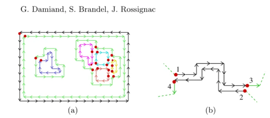
(a) 4 2 1 3 (b)
Fig. 2. (a) The linel combinatorial map of the topological map shown in Fig. 1. (b) An example of edge split to illustrate the links between l -darts and darts.
T corresponds to a region of I, and has a child for every region which is directly enclosed in it; the root of T being R0. (3) P is an interpixel matrix describing the geometry of C (its embedding ). In this matrix, a linel is on iff it is between two pixels that belong to two different regions; and a pointel is on iff it is incident to more that two linels on (except if a sequence of adjacent linels is a loop without any pointel on, one arbitrary pointel of the loop is switched on).
Links exist between the three elements of a topological map. For each dart d, region(d) is the region of T that contains dart d; pointel(d) is the pointel of P at the beginning of the oriented edge containing d (which is necessarily on); and linel(d) is the linel of P which is the first linel of the oriented edge described by d (which is also necessarily on). end-pointel(d) is the pointel at the end of the oriented edge containing d (which is also necessarily on). Lastly, for each region R, representative(R) is one dart of C belonging to the external boundary of R.
3
Linel Combinatorial Map
In this section, we introduce linel combinatorial maps, called l-maps, and show that it is possible to retrieve all the information of a topological map thanks to its corresponding l -map. In a second step, we show that l -maps can be represented implicitly by using only linels and local numbering of darts. Definition 1 (linel combinatorial map). Let T M = (C, T, P ) be a 2D topo-logical map, with C = (D, β1, β2). The linel combinatorial map of T M , called l-map, and denoted by Cl= (Dl, βl
1, β2l), is the 2-map obtained by splitting each edge of C so that each edge of Cl corresponds to a linel.
We call l-darts the darts of a linel combinatorial map, keeping word darts for the darts of the topological map. Since each l -dart d corresponds to a linel, linel(d) is now the unique linel of the edge containing d, and thus we have linel(d) =linel(βl
2(d)). An example of l -map is given in Fig. 2.
Let us consider D0 = {d ∈ Dl| pointel(d) is on in P } (the subset of l -darts having their pointel on, l -darts with red dots in Fig. 2). There is a one to one mapping between l -darts of D0 and darts of C (the minimal combinatorial map of T M ). Indeed, all darts in C are associated with pointels on; and insertion
operation does not switch any new pointel on. In the following of this paper, we use this one to one mapping to simplify our notations, denoting d both for an original dart in C and for its corresponding l -dart in Cl.
The following relationships between βi mappings and βl
i mappings can be given knowing that each edge in C is split in several unit edges in Cl, and that all new l -darts have their pointel off : ∀d ∈ Do:
– β1(d) = βl
k
1 ◦ β1l(d), k ≥ 0 is the smallest integer such that βl
k
1 ◦ β1l(d) ∈ Do; – β2(d) = βl
k
0 ◦ β2l(d), k ≥ 0 is the smallest integer such that βl
k
0 ◦ β2l(d) ∈ Do. βlk
1 means apply β1l k times. Since β0= β −1
1 , we have β0(d) = β0l(d) ◦ βl
k
0 . These relationships are illustrated in the example given in Fig. 2(b). The initial edge made of the two darts {1, 2} is split in eighteen l -darts (black oriented segments in the figure). β1(1) = 3, the l -dart obtained from β1l(1) and using β1l eight times. When following this path of l -darts, all pointels are off (because the corresponding l -darts result of the split of the initial edge) except the last pointel of l -dart 3. Things are similar for β0(4) = 2, the l -dart obtained starting from βl
0(4) and using β0l eight times; and for β2(1) = 2, the l -dart obtained from βl
2(1) and using β0l eight times.
Algorithm 1: Compute β1(d) Input: d: a dart.
Output: β1(d). d0 ← βl
1(d);
while pointel(d0) is off do d0 ← βl
1(d0); return d0 These relationships give us directly the
three algorithms that take a dart d as pa-rameter and compute βi(d) by using only l -darts, βl
i mappings, and the test if a pointel is off . Algorithm 1 allows to com-pute β1(d). Note that this algorithm takes a dart d as input, and thus pointel(d) is on by definition. Algorithms to compute β0(d) and β2(d) are similar.
One major advantage of a linel combinatorial map, and its relationships with a corresponding topological map, is the possibility to be considered at two different layers. (1) We can use βi links and iterate through a l-map exactly as if it is were a topological map. This is useful to compute easily “topological information” as the number of times two regions are adjacent or to retrieve all the regions adjacent to a given one. (2) We can use the βl
i links that allow to iterate through the “geometry” of the topological map; for example to draw the contours of a region by iterating through all its linels.
4
Implicit Representation of Linel Combinatorial Map
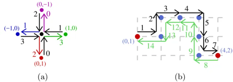
A l -dart d can be uniquely labeled by a pair (p, n), called descriptor , and denoted by desc(d). p is the end-pointel of d, and n is a number between 0 and 3: 0 for the bottom l -dart around p, 1 for the right l -dart, 2 for the top l -dart and 3 for the left l -dart (cf. Fig. 3(a)). Given desc(d), it is straightforward to retrieve pointel(d) and linel(d), which are directly encoded in the descriptor.
Now we define the three algorithms that compute the βl
i mappings by using only descriptors and test if a linel is on. Algorithm 2 allows to compute βl
(0,1) 0 2 3 0 2 (1,0) (−1,0) 1 (0,−1) 3 1 (a) (4,2) 1 2 3 4 5 6 7 14 11 10 9 8 12 13 (0,1) (b)
Fig. 3. (a) Descriptors for l -darts. Pointel (0, 0), in black, can be the pointel of four l -darts (black oriented segments), numbered locally from 0 to 3. The two l -darts to the right of this pointel have descriptors ((0, 0), 1) for the black l -dart and ((1, 0), 3) for the green l -dart. (b) Example to illustrate βl
i(d) computation. Pointels are drawn by
dots, red for pointels on, and blue for pointels off .
Algorithm 2: Compute βl 2(d). Input: ((i, j), n): descriptor of d. Output: descriptor of βl 2(d). switch n do case 0: j ← j + 1; n ← 2; case 1: i ← i + 1; n ← 3; case 2: j ← j − 1; n ← 0; case 3: i ← i − 1; n ← 1; return ((i, j), n) Algorithm 3: Compute βl 1(d). Input: (p, n): descriptor of d. Output: descriptor of βl 1(d). repeat n ← (n + 1) mod 4; until linel(p, n) is on; return β2(p, n)
This algorithm tests the four possible cases of l -darts, by using the local l -dart number, and returns directly the descriptor of βl
2(d) depending on each case. For example, if n = 0, βl
2(d) is the dart with local number 2 and having pointel (i, j + 1) as end-pointel.
In the example given in Fig. 3(b), βl
2(1) = 14 with desc(1) = ((1, 1), 3) and desc(14) = ((0, 1), 1) (case 3 in Algo. 2). Another example is βl
2(2) = 13 with desc(2) = ((1, 0), 0) and desc(13) = ((1, 1), 2) (case 0 in Algo. 2).
Algorithm 3 allows to compute βl
1(d). We turn around p, the end-pointel of d, in counter-clockwise order, until finding a linel on, l0, incident to p (same principle is used in digital boundary tracking, for example in [15]). We turn counter-clockwise because external contours are oriented clockwise, thus each l -dart has its region to its right (this is also true for inner contours because they are oriented counter-clockwise). β1l(d) is the l -dart having l0 as linel and pointel(d) as end-pointel: this is the l -dart β2(p, n). Note that by definition it is not possible to have only one linel on around a pointel. Thus starting from a l -dart (having hence its linel on l), we necessarily find a second linel on l06= l.
If we look at Fig. 3(a), we can observe that given a black l -dart d as input, βl
1(d) is necessarily a colored l -dart because d and its β1l have necessarily two dif-ferent end-pointels. For example βl
1(3) is necessarily one l -dart among ((0, 1), 2), ((1, 0), 3), ((0, −1), 0) and ((−1, 0), 1), depending on the local configuration of linels on around the black pointel.
In the example given in Fig. 3(b), βl
1(1) = 2 with desc(1) = ((1, 1), 3) and desc(2) = ((1, 0), 0). In the iteration around pointel (1, 1), the first linel on found, after linel(1), is linel(13) (desc(13) = ((1, 1), 2)); then βl
2(13) = 2 is returned. The algorithm to compute βl
0(d) is similar to the one that computes β1l(d) by reversing the orders of operations: we start to use β2(p, n), then iterate clockwise around the end-pointel of d.
5
Compact Encoding of l -maps
In this section, we present two compact encodings of linel combinatorial maps. Thanks to the relationships between l -maps and topological maps, the two en-coding of l -maps give us directly two compact enen-codings of topological maps. Note that in both cases, our encoding describes both the minimal combinato-rial map C and the interpixel matrix P of the topological map within the same data-structure, increasing even more the memory space reduction.
5.1 Matrix Representation
In this version, a l -map is encoded by a matrix M of three Booleans. M [i, j] encodes the configuration around pointel p = (i, j) by three Booleans: the first Boolean represents pointel p, the second Boolean the bottom linel of p and the third Boolean the right pointel of p. The value of each Boolean is false if the corresponding element is off , and true if it is on.
The main advantage of this encoding is to provide a direct access to each pointel/linel. Testing if pointel (i, j) is on is achieved directly by testing the first bit of M [i][j]. To test if linel ((i, j), n) is on, three cases must be considered. (1) If n = 0 or n = 1, testing if linel ((i, j), n) is on is directly the value of bit number n + 1 of M [i][j]. (2) If n = 2, testing if linel ((i, j), 2) is on is done by testing linel ((i, j − 1), 0). Indeed the top linel of pointel (i, j) is the same than the bottom linel of pointel (i, j − 1); but is only represented in pointel (i, j − 1). (3) Similarly, if n = 3, testing if linel ((i, j), 3) is on is done by testing linel ((i − 1, j), 1).
Another main advantage of this encoding is to allow simple modification op-erations. Indeed, it is enough to switch on/off some pointels/linels in order to modify the underlying topological map. Similarly, extraction algorithm becomes much simpler since it only consists to iterate through a labeled image and to switch on some pointels and linels based on local properties.
The main drawback of this representation is to “lose” some memory space to represent empty cells. The second representation proposed in this paper solves this drawback by do not representing at all the empty cells, but this is to the detriment of operations complexity.
5.2 Stacked Row Representation
The goal of this second version is to not store anything for empty cells. To do so, a l -map is now encoded by an array R of bitset. R[j] is the concatenation
of the encoding of all the active pointels of row number j. A pointel is active either if it is on, or if it is incident to one bottom, right or top linel on. Each active pointel is encoded by four Booleans: the first Boolean represents pointel p, the second Boolean the bottom linel of p, the third Boolean the right linel of p and the fourth Boolean the top linel of p. The value of each Boolean is false if the corresponding element is off , and true if it is on.
With this solution, each row is now encoded by a variable length representa-tion which has 4njbits, njbeing the number of active pointels in row number j. For this reason, it is no more possible to access directly, like for the previous so-lution, to a given pointel p = (i, j). We are going to explain now how to retrieve the neighbor pointels of p when we use this compact representation.
First, each l -dart descriptor ((i, j), n) is replaced by a descriptor, ((a, j), n), where a is the index of pointel p = (i, j) among the list of active pointels in the jth row (a = 0 for the first active pointel whatever its position, a = 1 for the second one, . . . ). This index allows to directly retrieve the four bits associated with pointel p which start at position 4a in R[j]. This index allows also to retrieve directly the previous and the next pointel of p in row j which are pointels (a − 1, j) and (a + 1, j). Note that these two formula are only valid if pointel p is active and its previous or next pointel is also active, but these formula will only be used in these cases.
Things are more complex to find pointels above and below p. Indeed, the number of active pointels in two consecutive rows are not necessarily the same, and thus it is not possible to use index a of row j to deduce index a0 in row j − 1 or j + 1. One solution is to encode, after each active pointel, the index of the pointels above and bellow it; but in this case the memory reduction compared to the matrix based solution becomes very small and is thus not really interesting. Our solution is to recompute these indices instead of storing them. Given an active pointel p = (a, j), the following principle is used to retrieve p0= (a0, j −1), the active pointel above p. (1) We count the number n1of top linels on, before or equal to p in row j. (2) We iterate through active pointels of row j − 1, starting from a0= 0, incrementing a0, and counting the number n2 of bottom linels on. When n1 = n2, the current pointel p0 = (a0, j − 1) is the active pointel above pointel p. Same principle is applied to retrieve the pointel below p by counting bottom linels on in row j, and top linels on in row j + 1.
Note that this encoding has some redundancy, because each vertical linel is stored twice: once as vertical linel above a given pointel (i, j); and once as vertical linel below pointel (i, j − 1). But this redundancy is necessary in order to retrieve up and down neighbors of a given pointel.
The main advantage of this solution is that no information is stored for non active pointels. Thus, the memory space is very compact and depends only on the size of the region boundaries, and not on the global size of the image. The main drawback is that the complexity to access to up and down neighbors pointel of a given pointel is no constant anymore but linear in number of active pointels. Testing if pointel (a, j) is on is achieved directly by testing the bit at position 4a in R[j]. Testing linels ((a, j), n) is also done directly when n = 0, 1 or 2: the
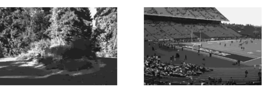
Fig. 4. Examples of 2D segmented images. (Left) arbogreens05. (Right) football05.
value of the linel is the bit at position 4a + n + 1 in R[j]. For n = 3, testing if linel ((a, j), 3) is on is done by testing linel ((a − 1, j), 1).
5.3 Links Between Darts and Regions
The two previous sections have shown how to retreive βil, pointel and linel of any l -dart by using only dart descriptors and tests if pointels and linels are on or off . In order to represent all the information of a topological map, it misses us to retrieve region(d) that gives the region that contains dart d.
To do so, an associative array, A, is added to our compact representation, that associates region identifiers to dart descriptors (e.g. a pointer or an index depending on how regions are stored). For each face of the l -map Cl, the minimal dart of the face is stored in A (minimal by using a lexicographic order on descriptors). To retrieve the region of a dart d, given by its descriptor, we iterate through all the darts of its face, using β1, until going back to d, and keeping the minimal dart, dmin, encountered during this walk. The region of d is directly obtained by A[dmin].
This solution has the main advantage to not require a big memory space since there is only one entry in A for each face of Cl. Its main drawback is the complexity of the operation to retrieve region(d) which is no more in constant time but linear in number of l -darts of the face containing d, plus the complexity to retrieve dmin in A. This complexity is linear in number of faces of Cl, #f , when A is represented by an array, is in log(#f ) when A is sorted, and is in average constant time if A is represented by a hash map.
6
Experiments
We have implemented our two compact representations of l -maps and compared memory spaces and computation times of our two solution (referenced in the following as compact storage with matrix or stacked row representation) with a classical implementation of 2D topological maps based on darts and pointers (referenced in the following as classical storage). We have used 224 images from [16] (arborgreens, cherries, football, greenlake and swissmountains classes) after a segmentation pre-processing. All these images have same resolution 756×504 (see two images in Fig. 4). We performed all benchmarks on the same computer, an Intel core-i7 4790 4-cores 3.6GHz with 32Go RAM.
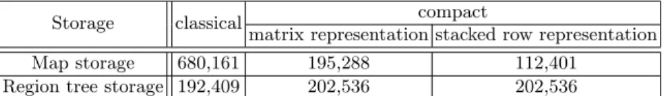
We have first compared the memory space used by the three versions (see table 1). On average for all input images, the memory space used for regions tree is about the same for the three versions. In classical storage, each representative dart is stored as a pointer (8 bytes in 64bits architectures), while in compact storage, each dart is stored as a descriptor (2 integers and a character, that is 9 bytes), explaining the small difference between both implementations.
Storage classical compact
matrix representation stacked row representation Map storage 680,161 195,288 112,401
Region tree storage 192,409 202,536 202,536 Table 1. Mean of used memory space (Bytes) with 224 images.
The memory space used for the 2-map in compact storage with a matrix is about 3 times smaller than in classical storage, and compact storage with stacked row is about 2 times smaller than the one using a matrix. These dif-ferences are more important in particular cases. For example, if the number of regions is small compared to the image size, the map size using stacked row rep-resentation can be 20 times smaller than one using matrix reprep-resentation. More precisely, since we store one pointel for each pixel in the matrix and we store only active pointels in the stacked row, the memory space reduction between both representations depends of the ratio between active pointels and all pointels. Similarly, the performances in terms of memory space of our three implementa-tions strongly depend of the image contents: the memory space reduction of our compact representations is better for topological map having many small darts than for images having large regions represented by only few darts.
Second, we have compared computation times (see table 2). Accesses to all elements of a topological map are in constant time for classical storage. For matrix representation, region(d) is linear in number of dart per face, and the complexity of βi mapping is linear in number of linels of the edge. For stacked row representation, the complexity of βi mapping depends also on the number of active pointel of traversed rows. This explains why times are generally faster with classical storage than with our compact storages.
Storage classical compact
matrix representation stacked row representation
Map extraction 91.6 10.2 66.7
Region tree building 0.5 38.9 637.1 All regions traversal 2.1 1.7 20.3
Segmentation 0.3 3.9 40.0
We have analyzed the computation time for building topological maps from labeled images. This step is much faster with compact storage than with clas-sical storage because compact storage computes only interpixel matrix, while classical storage computes additionally the 2-map. However, computation of the enclosure tree is faster with the classical representation due to the use of many βi operations.
Then, we have analyzed the computation time of two operations that iterate through a topological map T M . First we iterate through all regions of T M , and for each region R, we iterate through all its boundaries (as would do a method to visualize T M ). In this case, the matrix representation is the fastest method because we directly iterate through l -darts, while with the classical representation we need to iterate through T M then to each linel of each dart (but the difference is very small). As planned, the stacked row representation is slower due to the additional time required by the βi operations.
The second operation analyzed consists in iterating through all regions of T M , and for each region R, through each dart in its boundaries. For each dart d, we test the color difference between region(d) and region(β2(d)) and count as many differences are smaller than a given threshold (this is the first step of a re-gion growing segmentation). Here, the method using the classical representation is about 10 times faster than method the method using the matrix representa-tion, itself 10 times faster than the method using the stacked row representation. Our two compact representations give very good results in term or memory space occupation. Of course this is to the detriment of the complexity of opera-tions. But even with the stacked row representation, our results show that these complexities are still good enough to allow to process big images. And moreover, some operations are even faster than with the classical representation.
7
Conclusion
In this paper, we have proposed two compact representations of topological maps, solving the main drawback of these models which was the big memory space required to store them. These compact representations are based on the notion of linel combinatorial map and on relationships between darts and βilinks of the topological map, and l -darts and βl
i links of the l -map. The first representation, based on an interpixel matrix, allows direct access to each interpixel element and simplifies the modification of the topological map. The second representation is very compact, avoiding to represent empty elements, but implies a bigger complexity of operations. Users can choose between these two representations depending on their priorities.
As future work, we plan to integrate modification algorithms in both pro-posed representations, like split and merge methods. It could be interesting to study the impact of the second representation on the computation time of these methods. Some algorithms should perhaps be modified in order to improve their complexities in this specific case. We plan to study other representations more compact than the matrix while trying to decrease the complexity of operations.
We also would like to decrease the memory space used by the region tree. Lastly, we want to extend these compact representations in 3D.
References
1. Esther Ant´unez, Rebeca Marfil, Juan Pedro Bandera Rubio, and Antonio Bandera. Part-based object detection into a hierarchy of image segmentations combining color and topology. Pattern Recognition Letters, 34(7):744–753, 2013.
2. J.P. Braquelaire, P. Desbarats, J.P. Domenger, and C.A. W¨uthrich. A topological structuring for aggregates of 3D discrete objects. In Proc. of GbRPR, pages 193– 202, Austria, May 1999.
3. L. Brun, J.-P. Domenger, and J.-P. Braquelaire. Discrete maps: a framework for region segmentation algorithms. In Proc. of GbRPR, Lyon, Apr. 1997. IAPR-TC15. published in Advances in Computing (Springer).
4. L. Brun and J.P. Domenger. A new split and merge algorithm with topological maps and inter-pixel boundaries. In Proc. of WSCG, pages 21–30, Feb. 1997. 5. L. Brun and W.G. Kropatsch. Contraction kernels and combinatorial maps.
Pat-tern Recognition Letters, 24(8):1051–1057, 2003.
6. G. Damiand, Y. Bertrand, and C. Fiorio. Topological model for two-dimensional image representation: Definition and optimal extraction algorithm. Computer Vi-sion and Image Understanding, 93(2):111–154, Feb. 2004.
7. G. Damiand and D. Coeurjolly. A generic and parallel algorithm for 2D digital curve polygonal approximation. Journal of Real-Time Image Processing, 6(3):145– 157, Sep. 2011.
8. G Damiand and P. Lienhardt. Combinatorial Maps: Efficient Data Structures for Computer Graphics and Image Processing. A K Peters/CRC Press, Sep. 2014. 9. G. Damiand, S. Peltier, and L. Fuchs. Computing homology for surfaces with
gen-eralized maps: Application to 3D images. In Proc. of ISVC, volume 4292 of LNCS, pages 235–244, Lake Tahoe, Nevada, USA, Nov. 2006. Springer Berlin/Heidelberg. 10. C. Fiorio. A topologically consistent representation for image analysis: the frontiers topological graph. In Proc. of DGCI, number 1176 in LNCS, pages 151–162, Lyon, France, Nov. 1996.
11. R. Goffe, G. Damiand, and L. Brun. A causal extraction scheme in top-down pyramids for large images segmentation. In Proc. of SSPR, volume 6218 of LNCS, pages 264–274, Cesme, Izmir, Turkey, Aug. 2010. Springer Berlin/Heidelberg. 12. X. Jiang and H. Bunke. Marked subgraph isomorphism of ordered graphs. In Proc.
of ICAPR, volume 1451 of LNCS, pages 122–131, 1998.
13. V.A. Kovalevsky. Finite topology as applied to image analysis. Computer Vision, Graphics, and Image Processing, 46:141–161, 1989.
14. W.G. Kropatsch and H. Macho. Finding the structure of connected components using dual irregular pyramids. In Proc. of DGCI, pages 147–158, Sep. 1995. 15. J.-O. Lachaud. Coding cells of digital spaces: a framwork to write generic digital
topology algorithms. In Proc. of IWCIA, volume 12 of ENDM, Palerme, Italy, 2003. Elsevier.
16. Y. Li and L. G. Shapiro. Object and concept recognition for content-based image retrieval. http://www.cs.washington.edu/research/imagedatabase/.
17. P. Lienhardt. Topological models for boundary representation: a comparison with n-dimensional generalized maps. Computer Aided Design, 23(1):59–82, 1991. 18. A. Rosenfeld. Adjacency in digital pictures. Information and Control, 26-1:24–33,