HAL Id: hal-00180600
https://hal.archives-ouvertes.fr/hal-00180600
Submitted on 19 Oct 2007
HAL is a multi-disciplinary open access
archive for the deposit and dissemination of
sci-entific research documents, whether they are
pub-lished or not. The documents may come from
teaching and research institutions in France or
abroad, or from public or private research centers.
L’archive ouverte pluridisciplinaire HAL, est
destinée au dépôt et à la diffusion de documents
scientifiques de niveau recherche, publiés ou non,
émanant des établissements d’enseignement et de
recherche français ou étrangers, des laboratoires
publics ou privés.
wavelet features
Bin Luo, Jean-François Aujol, Yann Gousseau, Saïd Ladjal
To cite this version:
Bin Luo, Jean-François Aujol, Yann Gousseau, Saïd Ladjal. Indexing of satellite images with different
resolutions by wavelet features. IEEE Transactions on Image Processing, Institute of Electrical and
Electronics Engineers, 2008, 17 (8), pp.1465-1472. �hal-00180600�
Indexing of satellite images with different
resolutions by wavelet features
Bin Luo, Jean-Franc¸ois Aujol, Yann Gousseau, Sa¨ıd Ladjal
Abstract— As many users of imaging technologies, space
agencies are rapidly building up massive image databases. A particularity of these databases is that they are made of images with different but known resolution. In this paper, we introduce a new scheme allowing to index and compare images with different resolution. This scheme relies on a simplified modeling of the acquisition process of satellite images and uses continuous wavelet decompositions. We establish a correspondance between scales that permits to compare wavelet decompositions of images having different resolutions. We validate the approach through several matching and classification experiments, and show that taking the acquisition process into account yields better results than just using scaling properties of wavelet features.
I. INTRODUCTION
Spatial agencies are very rapidly building up massive databases of images. For example, the CNES (the French spatial agency) is receiving from its satellites several terabytes of data each day. Like most users of large databases, these in-stitutions need efficient tools to index and search their images. One particularity of satellite image databases, compared to e.g. natural images databases, is that they are made of images with different but known resolution1, depending on the satellite they originate from. In contrast, natural image databases are made of pictures with different resolutions but the relationship between the size of objects and pixels is unknown. Moreover, this quantity depends on the position of objects in the scene, so that the notion of resolution itself has little general meaning. This obvious fact made it necessary to develop scale invariant local features for many computer vision tasks, see e.g. [1]. For the indexing of texture, it makes sense to assume a uniform resolution through the image. Since this resolution is usually unknown, many scale invariant indexing schemes have been developed, see e.g. [2], [3], [4], and [5] for a review. Our purpose in this paper is quite different. First, the resolution of satellite images is usually a known parameter, at least if we neglect tilts of the optical device and assume that the scene being captured is approximately flat. Therefore, our goal is to be able to compare two images knowing their resolution difference. Second, a change in resolution is more complicated than just a scale change, since it usually involves an optical device and an imaging captor. In a previous work, [6], [7], this process was modeled as a convolution followed by a sampling and its effect on the computation of a characteristic scale was
B. Luo, Y. Gousseau and Sa¨ıd Ladjal are with GET/T´el´ecom Paris, CNRS UMR 5141 CNES-DLR-ENST Competence Centre, 46, rue Barrault, 75634, Paris Cedex 13, France.
J-F. Aujol is with CMLA, ENS Cachan, CNRS, UniverSud, 61 Av. President Wilson, F-94230 Cachan, France.
1By resolution, we mean the true pixel size in meter.
studied. In this paper, we make use of the same model and propose a scheme to compare features extracted from images at different resolutions. Observe that several works have been performed to extract image features that are invariant with respect to resolution changes [8], [9]. Again, our purpose is quite different since we wish to be able to compare images with different but known resolution.
Many features have been proposed to index satellite images [10], [11], [12], [13], [14]. In this work, we only consider mono-spectral images and classically choose to index them using texture features. In particular, wavelet features have been proved suitable for texture indexing or classification [15], [16], [17], [18], [19], [20], [21], [22]. Wavelet features have already been used for indexing remote-sensing images in [23]. The aim of the proposed approach is to investigate the interplay between resolution and wavelet features and to propose a scheme for the comparison of images with different resolutions. Preliminary results of the present work were presented in [24].
The plan of the paper is the following. In Section II a simplified model for the acquisition of satellite images is introduced. In Section III, we recall how the marginals of wavelet coefficients can be used for the indexing of images. In Section IV, a method is given to compare features extacted at different resolutions. In Section V, the dependence of features upon resolution is checked using satellite images from the CNES and the proposed scheme is validated through classification experiments. We then conclude in Section VI.
II. MODEL OF THE ACQUISITION PROCESS
A digital image fr at resolution r is obtained from a
continuous function f (representing the scene under study)
through an optical device and a digital captor. Neglecting contrast changes and quantization, the effect of the imaging device can be modeled as follows,
fr= ΠSr.(G ∗ f) + n,
where G is the convolution kernel, Sr ⊂ Z2 the sampling
grid at resolution r, ΠSr the Dirac comb on Sr and n the
noise. In what follows, we will take interest in the effect of the acquisition model on the wavelet coefficients offr. Therefore,
and assuming that we will neglect coefficients at the smallest scales, we will assume thatn = 0. Moreover, we will assume
that Sr = rZ2, that is a regular and square sampling grid
with step r. We thus neglect the satellite vibrations and scan
acquisition. Last and more importantly, according to [25], [26], the response of an ideal optic aperture could be very accurately
approximated by a Gaussian kernel. Therefore we will assume
that G is an isotropic Gaussian kernel, thus neglecting the
specificity of the satellite optics, the real response of the captor and motion blur. This is probably the strongest assumption made. The motivation behind it is mainly the tractability of forecoming computations, as will become clear soon. Last, we assume that the standard deviation of the kernel is proportional to the resolution. In the experimental section, we will check that these assumptions are not too restrictive by considering realistic satellite images. To summarize, we assume the fol-lowing acquisition model :
fr= Πr.(f ∗ krp), (1) where kσ(x, y) = 1 2πσ2exp µ −x 2+ y2 2σ2 ¶ , (2)
Πris the Dirac comb on rZ2, that is,
Πr=
X
i,j∈Z
δ(ir,jr),
and the parameter p is a characteristic of the acquisition
process.
III. WAVELET FEATURES FOR TEXTURE INDEXATION
Based on empirical observations, Mallat [27] proposed to model the marginals of wavelet coefficients of natural images by Generalized Gaussian Distributions (GGD). That is, writing
h for the density of the distribution of coefficients at some
scale and orientation,
h(u) = Ke−(|u|/α)β. (3)
It is shown in [15], [16], [17] that the parameters α and β of
GGD can be used as efficient features for texture indexing and classification. It is possible to compute these parameters from the estimation of the first and second order moments of |u| [27]: we denote them respectively bym1=R |u|h(u)du and
m2=R u2h(u)du. More precisely, m1= αΓ(2/β)Γ(1/β)−1
andm2= α2Γ(3/β)Γ(1/β)−1.
In this paper, for simplicity, we address the problem of relating features m1 andm2 to resolution changes. Adapting
the results to α and β is then straightforward. This can
be useful when using the Kullback-Leibler distance in a classification task, see [16].
In order not to be restricted to dyadic resolution changes, continuous wavelet transform [28] is used instead of the more classical discrete wavelet transform. Moreover, we consider
mother wavelets obtained as derivatives of a Gaussian kernel
in horizontal, vertical and diagonal directions. This important assumption is motivated by the simplified model for resolution changes presented in the previous section, as will be shown by the computations of Section IV-A.
Figure 1 shows a histogram of absolute values of wavelet coefficients, illustrating the soundness of the use of GGDs to model such distributions.
(a) Marseille 0 5 10 0 0.05 0.1 0.15 α = 2.61,β = 1.2626 (b) Histogram
Fig. 1. (a) Image of Marseille at resolution0.707m ( c°CNES); (b)
His-togram (blue bars) of wavelet coefficients of image (a) at scale5 (horizontal)
and the approximation by GGD (red curve).
IV. WAVELET FEATURES AND RESOLUTION CHANGES
A. Resolution Invariance
a) Notations: The discrete version of the Gaussian kernel
with standard deviationt (t being given in pixels) is denoted by ˜
kt. Let us define the discrete wavelet coefficient as (recall that
the wavelets we use are derivatives of the Gaussian kernel):
wq,r,t= ∆q˜kt˜∗fr= ˜kt˜∗∆qfr (4)
where q ∈ {0, 1, 2, 3}, ∆q stands for the difference between
adjacent pixels in the horizontal (q = 0), vertical (q = 1) or
diagonal (q = 2, 3) direction, and ˜∗ stands for the discrete
convolution operation.
b) Resolution invariance: Recall that the imagefrat
res-olutionr is obtained by fr= Πr.(krp∗ f). From Equation (4)
, we therefore have:
wq,r,t = ˜kt˜∗∆qΠr(krp∗ f) (5)
≈ ˜kt˜∗Πr{r∂q(krp∗ f)}.
The last approximation will be detailed in the appendix. Next, we assume that the inversion between convolution and sub-sampling is licit for non-aliased images such askσ∗f
whenσ is at least, say, r/2. The validity of this assumption on
real images has been checked in [7]. Assuming that ˜kt≈ krt
(see [7]), and that the continuous and discrete convolutions are equivalent, we have:
wq,r,t≈ rΠr.(krt∗ krp∗ ∂qf ). (6)
Using the semi-group property of the Gaussian kernel, it can be deduced that:
wq,r,t
r ≈ Πr.(kr√t2
+p2∗ ∂qf ). (7)
The accuracy of this approximation will be computed in the appendix.
Assume now that we have two images fr1 and fr2 of the
same scene at resolutions r1 and r2. ¿From (7), we deduce
that if we choose scalest1 andt2 such that:
r1 q t2 1+ p2= r2 q t2 2+ p2 (8) we have: m1(q, r1, t1)/r1≈ m1(q, r2, t2)/r2 (9) m2(q, r1, t1)/r12≈ m2(q, r2, t2)/r22 (10)
with m1(q, r, t) = 1 nr X |wq,r,t|, m2(q, r, t) = 1 nr X |wq,r,t|2,
where nr is the size of the discrete image fr and the sum
is taken over the image domain (notice that, since we use a continuous wavelet transform, w has the same size as fr).
These equalities (Formula (9) and (10)) will permit to compare wavelet features originating from f1 andf2. In what follows,
we denote by Θq,r,t = {m1(q, r, t), m2(q, r, t)} the wavelet
features at scale t and direction q extracted from fr.
c) Remark about the naive choice p = 0.0: A naive
assumption could be drawn that for the same scene f , if we
keep
r × t = C (11)
where C is a constant, the parameter set will also be constant
(after the correct normalization). However, this assumption is not sufficient because it approximates the resolution change by a simple zoom, which is not consistent with the acquisition process modeled in Section II. We will see in Section V that such a naive choice leads to poor numerical results compared with the use of Equation (8). In what follows, we will call ”naive choice” the use ofp = 0 in Equation (8).
d) Tuning ofp: To use Equation (8), one needs to know
the value ofp. This is a characteristic of the acquisition process
(see Equation (1)). This can therefore be tabulated once for each satellite. Observe that if one considers two images fr1
and fr2 with different resolutions, it is very likely that they
originate from different satellites and that the corresponding values ofp be different. In this case, writing pifor the value of
p corresponding to resolution ri (i = 1, 2) it is straightforward
to show that Equation (8) can be generalized to
r1 q t2 1+ p21= r2 q t2 2+ p22. (12)
This equality again ensures that approximations (9) and (10) will hold and permits the comparison of wavelet features from
fr1 and fr2. In what follows, for the sake of simplicity, we
will assume that p1= p2 and therefore use Equation (8).
B. Wavelet features and resolution
As explained in the introdution, the aim of this paper is to propose a way to compare the features originating from two images with different and known resolutions. One way to achieve this is to modify the features (i.e. the first and second order momentsm1 andm2) extracted at resolutionr1
to compare them (depending on r2 andr1) with the features
extracted at resolutionr2. Assume that we havefr1 the image
at resolutionr1of a given scene, and that we want to predict its
features at resolutionr2. From Equations (7)–(10), we deduce
the following scheme:
• Compute the wavelet coefficients forfr1 at scalesti,i =
1, 2, 3, . . . , N ;
• Estimate the parameters Θq,r1,ti from the wavelet
coef-ficients at scales ti for resolution r1 ;
• For resolutionr2, compute the scalest0i corresponding to
ti according to (see Equation (8))
t0i= s r2 1 r2 2 (t2 i + p2) − p2 (13) • Define ˜Θq,r2,t0i= Θq,r1,ti at scalest0i.
By using such an algorithm, it is now possible to compare images taken at different resolutions and, for instance, to train classification methods on a set of images at only one resolution and to apply the recognition criteria to images at different resolutions.
V. EXPERIMENTS AND RESULTS
A. Image database
In the following sections, we experimentally validate the proposed scheme for comparing wavelet features. These exper-iments are carried on an image database provided by the CNES (the French spatial agency). This database is made of various scenes (such as fields, forests and cities). Each scene has been acquired as an aerial image at resolution0.25m. Then, for each
scene, the CNES has simulated images at various resolutions, using realistic satellite modeling. The available resolutions range from0.5m to 4m, according to a geometric progression
with ratio21/6. In Figure 2 some examples of the images from
the database are shown. It is important at this point to note that convolution kernels used by the CNES are not Gaussian. However, we will see that the approximate acquisition model of Section II yields good numerical results. In what follows, we will use the acquisition model (1) with a value p = 1.3.
This value has been chosen as the value yielding the best numerical results (among values ranging from 1 to 2 by steps of 0.1) and also corresponds to a rough approximation of the kernel used by the CNES.
B. Validity of the prediction scheme
First, we check the validity of Formula (8), (9) and (10) by plotting numerical values of featuresm1 andm2.
In Figures 3 (d)-(f) (resp. (g)-(i)) graphs of m1(q, r, t)/r
(resp.m2(q, r, t)/r2) as functions ofr are presented when rt
is kept constant (that is when using the naive normalization of Equation (11)) and when rpt2+ p2 (here p = 1.30)
is kept constant (see Equation (8)). The resolution r ranges
from 0.50m to 4m. For the image at resolution 0.50m (the
highest available resolution), m1 and m2 are computed at
scale 16 in the horizontal direction. It may be seen that
using Equation (11) (that is forgetting the convolution step in the model of resolution change) does not yield a constant parameter set, especially when the resolution change is large. In such cases, one must use Equation (8) to compare features. Next, and for various scales, we compare values of m1
and m2 computed on an image with resolution 3.175m to
values of m1 and m2 computed on a image of the same
scene with resolution1m and then predicted for a resolution
of 3.175m. Figures 4 (a)-(c) (resp. (d)-(f)) show the values
of m1 (respectively m2) at various scales (scale is on the
(a) (b) (c) (d)
(e) (f) (g) (h)
(i) (j) (k) (l)
(m) (n) (o) (p)
(q) (r) (s) (t)
Fig. 2. Image samples from the database provided by the CNES: (a)-(d) Images at resolution0.5m; (e)-(h) Images at resolution 1.0m; (i)-(l) Images
at resolution2.0m; (m)-(p) Images at resolution 3.175m; (q)-(t) Images at
resolution4.0m; ¿From left to right, classes of the images are: city, field,
forest and sea.
(a) (b) (c) 0.5 1 1.5 2 2.5 3 3.5 4 0 0.1 0.2 0.3 0.4 0.5 0.6 0.7 0.8 0.9 resolution(m) m 1 /r rou11−m1− 0.5 1 1.5 2 2.5 3 3.5 4 0 0.2 0.4 0.6 0.8 1 1.2 resolution(m) m 1 /r didrai218−m1− 0.5 1 1.5 2 2.5 3 3.5 4 0 0.2 0.4 0.6 0.8 1 1.2 1.4 1.6 resolution(m) m 1 /r mar05−m1− (d) (e) (f) 0.5 1 1.5 2 2.5 3 3.5 4 0 0.2 0.4 0.6 0.8 1 1.2 1.4 1.6 1.8 2 resolution(m) m2 /r rou11−m 2− 0.5 1 1.5 2 2.5 3 3.5 4 0 0.2 0.4 0.6 0.8 1 1.2 1.4 resolution(m) m2 /r didrai218 −m2− 0.5 1 1.5 2 2.5 3 3.5 4 0 0.5 1 1.5 2 2.5 3 resolution(m) m2 /r mar05 −m2− (g) (h) (i)
Fig. 3. (a)-(c) Three images ( c°CNES); (d)-(f) graphs ofm1(q, r, t)/r (with
q = 0) as a function of r; (g)-(i) graphs of m2(q, r, t)/r2(withq = 0) as
a function ofr. On all these graphs, solid lines correspond to the case where r2pt2+ p2is kept constant (withp = 1.3), and dashed lines correspond to
the case the case wherert is kept constant.
1.5 2 2.5 3 3.5 4 4.5 5 5.5 0 0.5 1 1.5 2 2.5 3 3.5 roujan110 −− m 1 scale m1 moment 1.5 2 2.5 3 3.5 4 4.5 5 5.5 0 0.5 1 1.5 2 2.5 3 3.5 4 4.5 didrai218 −− m 1 scale m1 moment 1.5 2 2.5 3 3.5 4 4.5 5 5.5 0 1 2 3 4 5 6 7 mar05 −− m 1 scale m1 moment (a) (b) (c) 1.5 2 2.5 3 3.5 4 4.5 5 5.5 0 5 10 15 20 25 roujan110 −− m2 scale m2 moment 1.5 2 2.5 3 3.5 4 4.5 5 5.5 0 5 10 15 20 25 didrai218 −− m2 scale m2 moment 1.5 2 2.5 3 3.5 4 4.5 5 5.5 0 10 20 30 40 50 60 mar05 −− m2 scale m2 moment (d) (e) (f)
Fig. 4. Values ofm1((a)-(c)) and ofm2((d)-(f)) for various scales (scale
corresponds to the horizontal axis). In solid red line are displayed the values computed directly on images with resolution3.175m (the ground truth in this
experiment). In solid blue line, are displayed the values first computed on the images with resolution1m and then predicted using the scheme presented in
Section IV-B. Both solid lines almost perfectly coincide, showing the accuracy of the scheme. Dash lines show the results obtained by using the scheme proposed in Section IV-B but replacing Equation (13) witht0
i= r1ti/r2(the
naive normalization).
On the same figure,m1(resp.m2) predicted from a resolution
of 1m for a resolution of 3.175m according to the scheme
presented in Section IV-B are displayed by a solid red line. The two solid lines almost perfectly coincide. In dashed line, are plotted the values ofm1(respectivelym2) predicted from
a resolution of 1m for a resolution of 3.175m by the same
scheme of Section IV-B, except that Equation (13) is replaced byt0
i= r1ti/r2. This corresponds to what we called the naive
choice, neglecting convolutions in the resolution change. It can be seen that in this case, the guessed values ofm1andm2are
less accurate, especially for small scales. These experiments validate the scheme proposed in Section IV-B and suggests that it is necessary to take into account the convolution step in resolution changes to be able to compare features computed on images with different resolution. The next section investigates how the accuracy of the proposed scheme permits the classification of images at different resolutions.
C. Classification
a) Classified database: We have manually built a
clas-sified database based on the sequences of images provided by the CNES. This database contains366 scenes observed on
urban areas (Marseille and Toulouse), rural areas (Roujan), forests (Didrai) and the sea. For each scene, there are 5
dif-ferent images corresponding to 5 difdif-ferent resolutions (0.5m, 1m, 2m, 3.175m and 4m). The scenes are manually divided
into 4 sets: city (199 scenes), fields (134 scenes), forests (23
scenes) and sea (10 scenes).
b) Experiment: The first experiment carried out on this
database is classification. Images at the resolution of4m are
used as a learning set for training the classifier. The aim is to find the classes of the images at resolutions other than
4m. Wavelet features (m1andm2) are at first extracted from
all the images by applying Gaussian derivatives at different scales in4 directions (horizontal, vertical and diagonal). The
TABLE I
CLASSIFICATION RESULTS OBTAINED WITH WAVELET FEATURES EXTRACTED IN4
DIRECTIONS AT21SCALES(t = {2i/6|i = 0, 1, . . . , 20}). THE LEARNING SET IS MADE OF IMAGES AT RESOLUTION4m.
Resolution error (p = 1.3) error (p = 0)
0.5m 0.00% 21.86% 1m 0.00% 19.95% 2m 0.00% 10.66% 3.175m 0.00% 1.91%
TABLE II
CLASSIFICATION RESULTS OBTAINED WITH WAVELET FEATURES EXTRACTED IN4
DIRECTIONS AT3SCALES(t = 1, 2, 4). THE LEARNING SET IS MADE OF IMAGES AT RESOLUTION4m.
Resolution error (p = 1.3) error (p = 0)
0.5m 0.55% 26.50% 1m 0.00% 24.59% 2m 0.00% 12.84% 3.175m 0.27% 4.92%
features extracted from the images at a resolution of 4m
over 21 scales (t = {2i/6, i = 0, 1, . . . , 20}) are used to
train the classifier. Therefore the dimension of the feature space is 2 × 4 × 21 = 168. The features extracted from the other resolutions are predicted for 4m by using the scheme
presented in Section IV-B. For comparison, we set the valuep
respectively equal to 1.3 (using the acquisition model) and 0.0 (the naive approach). We then classify the images at
resolutions other than 4m with the predicted features.
The classifier we used is simply the nearest neighbor classification algorithm. For a given image A, the classifier search for its nearest neighbor B in the training set and affect to A the class of B. As a distance between features, we use the Euclidean distance, after normalizing each coordinate by its variance.
c) Results: The classification results are shown in Tab. I.
It can be observed that with the naive approach, the classifica-tion errors increase rapidly when the resoluclassifica-tion gets away from
4m. This shows numerically that the naive approach (p = 0) is
not a good choice for classification purpose. On the contrary, when the acquisition model is taken into consideration (i.e.
p = 1.3), there is no error. This is due to the fact that the
prediction scheme is very accurate, as we have shown in Section V-B. Errors are small enough not to switch from one class to another when changing the resolution.
d) Influence of the number of features: The classification
results presented in Table I are obtained from features in a space with relatively large dimension (168 values for each
image). We therefore study the effect of a dimension reduction. In Table II are shown the classification results obtained when performing the same experiment as in Table I, using the wavelet features (m1andm2) at only 3 scales (t = 1, 2, 4). In
this case the dimension of the feature space is 2 × 4 × 3 = 24 and it can be observed that the errors remain similar.
e) Comparison with other features: In order to further
investigate the effect of resolution changes on classification tasks, we perform an experiment using Haralick features.
TABLE III
CLASSIFICATION RESULTS OBTAINED WITHHARALICK FEATURES. THE DISTANCE PARAMETER FOR CALCULATING CO-OCCURRENT MATRICES VARIES ACCORDING TO
THE RESOLUTION OF IMAGE. THE LEARNING SET IS MADE OF IMAGES AT RESOLUTION4m.
Resolution distance error 0.5m 24 31.9%
1m 12 22.4% 2m 6 13.6% 3.175m 4 10.1%
Haralick [29] has proposed features based on the statistics of co-occurrence matrices of images. These features are proved to be very efficient for indexing textures. Co-occurence matrices are defined as the empirical joint distribution of the gray values of pixels in some direction θ and at some distance d. The considered directions are horizontal, vertical and two
diagonal directions. The distance between the pixel pairs can be considered as a scale parameter. For images at different resolutions, it is therefore natural to compute co-occurrence matrices with different distances. In our experiment, we set
d = 3, 4, 6, 12, 24 respectively for images at resolutions 4m, 3.175m, 2m, 1m and 0.5m. These values ensure that d×r is a
constant. The Haralick features are composed of13 statistical
values calculated from each matrix and the mean and standard deviation values through the four directions. Therefore the total feature dimension is(4 + 2) × 13 = 78.
Figure III shows the classification results obtained with Haralick features. Our purpose here is not to compare directly these results with the results obtained in the previous section. Indeed, results obtained with wavelet features are better, but we did not take full advantages of co-occurrence matrices since only one scale is used for each image. The interesting point is to notice how fast the classification results decrease with the change of resolution, therefore showing the inability of Haralick features to handle such changes. Observe that the approach taken here is similar to the naive choice of previous sections (approximating a resolution change through a zoom). Due to the non-linear nature of co-occurrence matrices, the approach proposed in the case of wavelet features is not adaptable to Haralick features.
D. Image Matching
In this subsection, we carry out a more difficult experiment than in the previous subsections. For each image at a resolution
of4m, we want to find the exact same scene from the images
at other resolutions with the help of wavelet features. The features are extracted and predicted as presented in Section IV-B. For an image at a resolution different from4m, we search
its nearest neighbor in the feature space among the set of images at4m. If the two images are of the same scene, it is
a correct match, otherwise it is an error. This is the same classification task as before, except that we consider each scene to be a class in itself.
In Table IV are displayed the matching results when using features over 21 scales (ti = 2i/6, i = 0, 1, ˙,20) and 4
TABLE IV
MISMATCHING PERCENTAGES WHEN USING WAVELET FEATURES EXTRACTED AT21
SCALES WITH4ORIENTATIONS.
resolution 0.5 1.0 2.0 3.175 p=1.3 4.1 0.27 0 1.64
p=0 81.97 79.51 65.57 34.97
TABLE V
MISMATCHING PERCENTAGES WHEN USING WAVELET FEATURES EXTRACTED AT3
SCALES WITH4ORIENTATIONS
resolution 0.5 1.0 2.0 3.175 p=1.3 11.2 4.64 1.09 9.29
p=0 95.90 96.45 92.62 62.02
orientations. In Figure V are displayed the matching results when using only3 scales (ti = 2i,i = 0, 1, 2).
It can be observed that:
• The errors increase considerably when compared to the classification results of the previous subsection, especially
when p = 0.0. This is due to the fact that in the image
database, there are many scenes of the same class which are very similar one to another. Therefore the points representing these images in the feature space are close one to another. As a consequence, a small error in the prediction causes an error in the image matching, in contrast with the classification case of Section V-C.
• The small errors in the casep = 1.3 confirm the accuracy
of the scheme.
VI. CONCLUSIONS AND PERSPECTIVES
In this paper, we have proposed a scheme for comparing wavelet features from images taken at different resolutions.
The acquisition of images is modeled by a convolution followed by a sampling. The scheme to compare wavelet features is based on this model and the semi-group property of the Gaussian kernel. We first checked experimentally the validity of this scheme and showed that the numerical accuracy is significantly improved compared to a naive approach where resolution change is simply modeled by a zoom. This approach is then applied for the classification of satellite images at several resolutions simulated by the CNES. Our approach improves significantly the accuracy of the classification. This fact is confirmed trough an image matching experiment.
The method presented in Section IV-B to compare wavelet features between images with different resolution is quite general. We applied it to images classification, but other tasks could benefit from this approach. For instance, the scale invari-ance of wavelet transformations has been applied to the fusion of aerial images having different resolutions [30][31][32]. None of these works takes into account the influence of the optics and captors on the change of resolution. We believe that the approach presented in Section IV could improve the precision of such fusions of images.
Acknowledgements: We thank Mihai Datcu, Alain Giros and Henri Maˆıtre for their advices and comments.
APPENDIX
In this appendix, we detail the approximation made in Equa-tion (5) and compute the error funcEqua-tions of the approximaEqua-tion made in Equation (6).
Recall that wq,r,t are the wavelet (Gaussian derivative)
coefficients extracted from fr at scale t and in direction q,
where fr is the digital image at resolution r obtained from
the continuous scene f . For clarity, we only consider the 1D
case. Recall Formula (5):
wq,r,t = ∆q˜kt˜∗Πr(krp∗ f)
= ˜kt˜∗∆qΠr(krp∗ f).
In the1D case, we have
wr,t= ˜kt˜∗∆xΠr(krp∗ f).
Writingg(x) = (krp∗ f)(x), we have
wr,t(x) = ˜kt˜∗∆xΠr(g(x))
= ˜kt˜∗(Πr(g(x + r) − g(x))),
and sinceg ∈ C1, we have
g(x + r) = g(x) + rg0(x) + o(r).
Therefore
wr,t ≈ ˜kt˜∗Πr(g(x) + rg0(x) − g(x))
= ˜kt˜∗Πr(rg0(x))
≈ r˜kt˜∗Πr(krp∗ f0(x)).
This is the approximation made in Equation (5). Next, we compute the error energy of the approximation made in Equation (6). For simplicity, we consider the resolutionr = 1.
We want to show that the energy of the error is small.
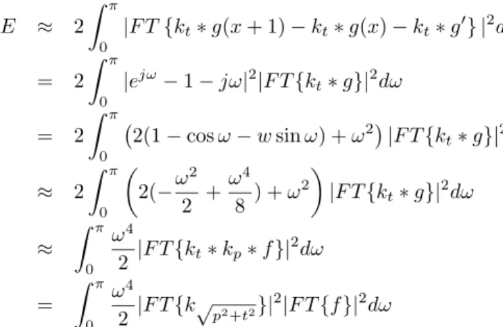
E = X|∆x˜kt∗ Π1(g) − Π1(kt∗ g0)|2 = Z |F Tn∆xk˜t∗ Π1(g) − Π1(kt∗ g0) o |2dω
whereF T (f ) is the Fourier transform of f . With the
approx-imationkt≈ Πr(krt), we have E ≈ Z |F T {∆xΠ1(kt∗ g) − Π1(kt∗ g0)} |2dω = Z |F T {Π1(kt∗ g(x + 1) − kt∗ g(x)) − Π1(kt∗ g0)} |2dω = Z |F T {Π1(kt∗ g(x + 1) − kt∗ g(x) − kt∗ g0)} |2dω
0 0.5 1 1.5 2 2.5 3 0 0.005 0.01 0.015 0.02 0.025 0.03 E function power spec
Fig. 5. Error function (E) and power spectrum of wavelet coefficients wr,t
in the frequency domain.
limited), therefore : E ≈ 2 Z π 0 |F T {k t∗ g(x + 1) − kt∗ g(x) − kt∗ g0} |2dω = 2 Z π 0 |e jω − 1 − jω|2|F T {kt∗ g}|2dω = 2 Z π 0 ¡2(1 − cos ω − w sin ω) + ω 2 ¢ |F T {kt∗ g}|2dω ≈ 2 Z π 0 µ 2(−ω 2 2 + ω4 8 ) + ω 2 ¶ |F T {kt∗ g}|2dω ≈ Z π 0 ω4 2 |F T {kt∗ kp∗ f}| 2dω = Z π 0 ω4 2 |F T {k√p2+t2}| 2 |F T {f}|2dω
Recall that t ≥ 1 and p = 1.3 in all our numerical experi-ments. Since the power spectrum of the image f is generally
decreasing, and ω24 is increasing, the worst case (which yields the largest error) is therefore |F T {f}|2= 1 for all ω, where
we have E ≈ Z π 0 ω4 2 |F T {k√12+1.32}| 2dω and E P |wr,t|2 ≈ 0.035
Figure 5 shows a plot ofE and the power spectrum of wavelet
coefficients wr,t in the frequency domain for the case where
|F T {f}|2= 1. In the worst case, the approximation made in
Equation (6) yields an energy error of 3.5% when compared
to the energy of the original wavelet coefficients. REFERENCES
[1] D.G. Lowe, “Distinctive image features from scale-invariant keypoints,”
International Journal of Computer Vision, vol. 60, no. 2, pp. 91–110,
2004.
[2] Fernand S. Cohen Zhigang Fan and M. A. Patel, “Classification of rotated and scaled textured images using gaussian markov random field models,” IEEE PAMI, vol. 13, no. 2, pp. 192–202, February 1991. [3] Jianguo Zhang and Tieniu Tan, “Affine invariant texture signatures,” in
ICIP, 2001.
[4] C. M. Pun and M. C. Lee, “Log-polar wavelet energy signatures for rotation and scale invariant texture classification,” IEEE PAMI, vol. 25, no. 5, pp. 590–603, 2003.
[5] J. Zhang and T. Tan, “A brief review of invariant texture analysis methods,” Pattern Recognition, vol. 35, pp. 735–747, 2002.
[6] B. Luo, J-F. Aujol, Y. Gousseau, S. Ladjal, and H. Maˆıtre, “Character-istic scale in satellite images,” in ICASSP 2006, 2006.
[7] B. Luo, J-F. Aujol, Y. Gousseau, S. Ladjal, and H. Maˆıtre, “Resolution independant characteristic scale dedicated to satellite images,” IEEE
Trans. on Image Processing, vol. 16, no. 10, pp. 2503–2514, 2007.
[8] Jan Flusser and Tomas Suk, “Degraded image analysis: An invariant approach,” IEEE PAMI, vol. 20, no. 6, June 1998.
[9] J. van de Weijer and C. Schmid, “Blur robust and color constant image description,” in International Conference on Image Processing, 2006. [10] A. Lorette, X. Descombes, and J. Zerubia, “Texture analysis through a
markovian modelling and fuzzy classification: Application to urban area extraction from satellite images,” International Journal of Computer
Vision, vol. 36, no. 3, pp. 221–236, 2000.
[11] G. Rellier, X. Descombes, F. Falzon, and J. Zerubia, “Texture feature analysis using a gauss-markov model in hyperspectral image classifica-tion,” IEEE Transactions on Geoscience and Remote Sensing, vol. 42, no. 7, pp. 1543–1551, 2004.
[12] M. Datcu, K. Seidel, and M. Walessa, “Spatial information retrieval from remote-sensing images. ii. information theoretical perspective,” IEEE
Trans. Geoscience and Remote Sensing, vol. 36, no. 5, pp. 1431–1445,
1998.
[13] K. Chen and R. Blong, “Identifying the characteristic scale of scene variation in fine spatial resolution imagery with wavelet transform-based sub-image statistics,” International Journal of Remote Sensing, vol. 24, no. 9, pp. 1983–1989, 2003.
[14] T. Gevers and H. Stokman, “Robust photometric invariant region detection in multispectral images,” IJCV, vol. 53, pp. 135–151, July 2003.
[15] D. Van Dyck G. Van de Wouwer, G. Scheunders, “Statistical texture characterization from discrete wavelet representations,” IEEE Trans. on
Image Processing, vol. 8, no. 4, pp. 592–598, 1999.
[16] Minh N. Do and Martin Vetterli, “Wavelet-based texture retrieval using generalized gaussian density and kullback-leibler distance,” IEEE
Transactions on Image Processing, vol. 11, no. 2, pp. 146–158, February
2002.
[17] J-F. Aujol, G. Aubert, and L. Blanc-F´eraud, “Wavelet-based level set evolution for classification of textured images,” IEEE Transactions on
Image Processing, vol. 12, no. 12, pp. 1634–1641, 2003.
[18] M. Unser, “Texture classification and segmentation using wavelet frames,” IEEE Transactions on Image Processing, vol. 4, no. 11, pp. 1549–1560, November 1995.
[19] H. Choi and R.G. Baraniuk, “Multiscale image segmentation using wavelet-domain hidden markov models,” IEEE Transactions on Image
Processing, vol. 10, no. 9, pp. 1309–1321, September 2001.
[20] G. Van de Wouwer, P. Scheunders, and D. Van Dyck, “Statistical texture characterisation from discrete wavelet representation,” IEEE IP, vol. 8, no. 4, pp. 592–598, 1999.
[21] J. Liu and P. Moulin, “Information-theoretic analysis of interscale and intrascale dependencies between image wavelet coefficients,” IEEE Transactions on Image Processing, vol. 10, no. 11, pp. 1647–1658,
November 2001.
[22] J.L. Chen and A. Kundu, “Rotation and gray scale transform invariant texture identification using wavelet decomposition and hidden markov model,” IEEE Transactions on Pattern Analysis and Machine
Intelli-gence, vol. 16, no. 2, pp. 208–214, February 1994.
[23] Soe Win Myint, Nina S.-N. Lam, and John M. Tyler, “Wavelets for urban spatial feature discrimination: Comparisons with fractal, spatial autocorrelation, and spatial co-occurence approaches,” Photogrammetric
Engineering and Remote Sensing, vol. 70, pp. 803–812, July 2004.
[24] B. Luo, J-F. Aujol, Y. Gousseau, and S. Ladjal, “Interpolation of wavelet features for satellite images with different resolutions,” in IGARSS, Denver USA, 2006.
[25] D.F. Ellliott, L.L. Hung, E. Leong, and D.L Webb, “Accuracy of gaussian approximation for simulating eo sensor response,” in Conference Record
of the Thirtieth Asilomar Conference on Signals, Systems and Computers 1996, 1996, pp. 868–872.
[26] B. Zhang, J. Zerubia, and J.C. Olivo-Marin, “Gaussian approximations of fluorescence microscope point-spread function models,” Applied Optics, vol. 46, no. 10, pp. 1819–1829, avril 2007.
[27] Stephane G. Mallat, “A theory for multiresolution signal decomposition: The wavelet representation,” IEEE PAMI, vol. 11, no. 7, pp. 674–693, July 1989.
[28] S.G. Mallat, A Wavelet Tour of Signal Processing, Academic Press, 1998.
[29] R.M. Haralick, K. Shanmugam, and I. Dinstein, “Textural features for image classification,” IEEE Transactions on Systems Man and Cybernetics, vol. SMC-3(6), 1973.
[30] Ranchin Thierry, “Remote sensing and image fusion methods: A comparison,” ICASSP 2006 Proceedings. 2006 IEEE International Conference on Acoustics, Speech and Signal Processing, 2006., vol. 5,
May 2006.
[31] Gang Hong and Yun Zhang, “High resolution image fusion based on wavelet and ihs transformations,” 2nd GRSS/ISPRS Joint Workshop on
Remote Sensing and Data Fusion over Urban Areas, 2003, pp. 99–104,
May 2003.
[32] N´unez J., Otazu X., Fors O., Prades A., Pala V., and Arbiol R., “Multiresolution-based image fusion with additive wavelet decompo-sition,” IEEE Transactions on Geoscience and Remote Sensing, May 1999.