HAL Id: hal-01446536
https://hal-mines-paristech.archives-ouvertes.fr/hal-01446536
Submitted on 26 Jan 2017HAL is a multi-disciplinary open access
archive for the deposit and dissemination of sci-entific research documents, whether they are pub-lished or not. The documents may come from teaching and research institutions in France or abroad, or from public or private research centers.
L’archive ouverte pluridisciplinaire HAL, est destinée au dépôt et à la diffusion de documents scientifiques de niveau recherche, publiés ou non, émanant des établissements d’enseignement et de recherche français ou étrangers, des laboratoires publics ou privés.
To cite this version:
Jean-François Agassant, Malcolm. R. Mackley. Principles of polymer processing modelling. NUMI-FORM 2016: The 12th International Conference on Numerical Methods in Industrial Forming Pro-cesses, The Minerals, Metals & Materials Society, Jul 2016, Troyes, France. pp.11002, �10.1051/mate-cconf/20168011002�. �hal-01446536�
aCorresponding author: [email protected]
Principles of polymer processing modelling
Jean-François Agassant1a and Malcolm. R. Mackley2
1
MINES ParisTech, PSL Research University, CEMEF, UMR CNRS 7635, 06560 Valbonne ,France
2
Department of Chemical Engineering and Biotechnology, University of Cambridge, UK
Abstract. Polymer processing involves three thermo-mechanical stages: Plastication of solid polymer granules or
powder to an homogeneous fluid which is shaped under pressure in moulds or dies and finally cooled and eventually drawn to obtain the final plastic part. Physical properties of polymers (high viscosity, non-linear rheology, low thermal diffusivity) as well as the complex shape of most plastic parts make modelling a challenge. Several examples (film blowing extrusion dies, injection moulding, blow moulding) are presented and discussed.
1 Introduction
Numerical modeling of polymer processing has now become an important tool in relation to the cost effective design and operation of polymer processes. In the past, the empirical development of new polymer grades has been motivated largely by searching for new or improved properties and it was assumed that the forming processes used to produce end products could be adapted through laboratory based adjustments made by simple trial and error. This worked effectively for a number of early cases; however sometimes it was discovered that new polymers with predicted "exceptional" properties were very difficult to process, either because the required pressure or torque could not be obtained with existing machines, or because the process exhibited flow or drawing instabilities at production rates inconsistent with their economic viability.
More recently, polymer producers have integrated the forming process into their development of new materials by using at an early stage of the development mini-processing machines (extruders or injection molding) that could discern potential processing problems using just a few hundred grams of polymer. Sometimes, the extrapolation to industrial size machines has proved uncertain, particularly because "scaling" does not obey the same scaling rules for mechanical and thermal behavior.
Numerical modeling, used initially in the field of injection mold design, has now become an important design aid tool in different sectors of the plastics industry, but it only makes sense to do this if the modeling is based on sound physical principles and the applied numerical techniques can capture the relevant process physics.
2 Fundamentals relevant to polymer
Processing modelling
Shaping thermoplastic polymers is a thermo-mechanical process which requires generally three successive steps: x Melting, that is to say the passage of the solid state, powder or granules, to a molten state in order to give a sufficiently fluid and homogeneous melt.
x Flow of the molten polymer under pressure
through a die or into a mold, shaping cooling, possibly coupled with drawing operations, biaxial stretching, blowing.
x Solidification into the final component shape and form.
The properties of the produced part will depend, of course, on the chosen polymer, but also on the "thermo-mechanical path" that was followed to shape the object. In the light of figure 1, it can be imagined that polymer processing is a problem of fluid mechanics coupled to heat transfer. In reality it is more complicated because rheology and heat transfer of thermoplastic polymers produce both experimental and modeling challenges.
Figure 1. General procedure for polymer processing
x At processing temperatures, molten polymers
generally have a viscosity as high as 103 Pas, which is a million times larger than water’s viscosity and this property has a number of significant consequences: the Reynolds number is low and generally below unity. As a consequence a molten polymer flow will never be turbulent, and often the inertial terms of the force balance equations can be neglected. The gravity force is negligible in most confined flows, however it may
become important in free surface processes as in film blowing, fiber spinning and extrusion blow molding for large hollow bodies.
Heating of the polymer by viscous flow dissipation can be very significant and this can be used with benefit for example in plasticization units: In many common extrusion operating conditions, energy introduced into the polymer by heat conduction and by viscous dissipation are of the same order of magnitude and therefore it is essential when modelling these situations to solve both the thermal and force balance coupled equations.
x Molten polymer present shear thinning as well as viscoelastic effects which lead to complex non-linear constitutive equations. The most sophisticated constitutive equation is not necessarily the most relevant or useful for modeling engineering processes. The choice depends on the process to be solved, on the type of flow, on the available computer facilities and, of course, on the available rheological measurements. If the objective of the calculation is to know the stress distribution, the orientation of macromolecules or of short glass reinforcing fibers, it is necessary to introduce a viscoelastic behavior law. If, however, the aim is only to establish pressure flow-rate relationships in a confined shear flow or shear dominant flow it is necessary to take into account accurately the shear rate and temperature dependence of the viscosity. In that kind of geometry, viscoelasticity modifies only marginally the velocity field and the normal stress at the wall. In an extensional flow with a free surface, it is usually essential to use a viscoelastic law because only this type of behavior is able to account for the often experimentally observed increase in extensional viscosity with the elongation rate.
x The low thermal conductivity of polymers as
well as the temperature dependence of the viscosity introduce specific problems which may need to be addressed when solving polymer processing problems. Heating by viscous dissipation is localized where both rate of strain and stress are important and the low thermal conductivity of polymer will consequently promote the existence of high thermal gradients. Given the risk of polymer degradation due to these localized overheating phenomena, this limits the amount of energy that can be provided by viscous dissipation and the flow rates that can be obtained.
3 Base equations and modelling
strategies
3.1 A set of ten base equations…
… has to be solved in a 3D geometry: a mass balance (generally, but not always, incompressible), three force balance equations where mass and inertia forces are
neglected, constitutive equations for the rheology ( 5 equations), a thermal balance equation.
3.2 Boundary conditions
In confined flows (extrusion dies, injection molds), it is generally assumed that the polymer adheres to the metal tool wall. Slip may occur when processing reinforced polymers, rubbers or PVC compounds. The problem is then to define a realistic sliding law. This gives rise, even today, to scientific debate. For standard thermoplastic polymers slip can also occur at high throughput; it is then usually associated with the existence of extrusion defects. In free surface flows (fiber spinning, blown film, for example), a velocity tangent at the free surface and a zero normal stress to this free surface are imposed.
In unsteady free surface flows (mold filling, but also blow molding), the stress component normal at the surface is again zero, but now the free surface propagates along the normal to this free surface.
Thermal boundary conditions can also present difficulties as the geometry of polymer processing equipment can be complex and wherever there is a free surface involved appropriate heat transfer coefficients must be chosen involving free or forced convection, radiation.
3.3 Model simplification
Solving the above full set of equations is still a very challenging numerical problem and so in the past it has been traditional to make wherever possible a number of approximations [1,2].
Geometric approximations consist for example in
unrolling the flow geometry. This is carried out to analyze the flow between the screw and the barrel of a single screw extruder (Tadmor and Klein [3]). They may also consist of decomposing a complex flow geometry into several more simple flow geometries where local mass balance and pressure equilibrium equations can be written (this will be described for simplifying a film blowing die).
Hydrodynamic lubrication or Hele-Shaw Approximations [4]: In many polymer processing
geometries, the transverse dimension of the flow is small compared to the other dimensions and slightly varies in the flow direction. Lubrication approximation helps to reduce the problem of solving 2D or 3D Stokes equations to a single pressure dependent equation.
Membrane approximation: When considering, for
example, the blowing of a membrane, it is assumed that the velocity components are uniform in the thickness.
Approximations can also be made to the thermal equation. For thin layer geometries an average
temperature balance equation may be written on a material volume. Dimensionless numbers (Cameron [5], Brinkman [6]) allow obtaining rapidly relevant order of magnitude values of the temperature field in most polymer processes.
3.4 Numerical schemes
In any three-dimensional flow there are ten equations that provide access to the ten unknowns that have to be solved. Several numerical methods are available.
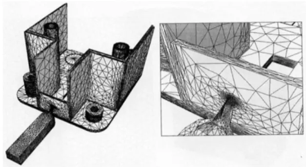
x In "direct" methods, a CAD definition of the die or mold geometry allows meshing the 3D flow volume and then solving the set of equations using generally finite elements. Meshing is a key point for obtaining an accurate result while controlling the computation time. Figure 2 presents the mesh of a complex cavity mold where capturing the flow in narrow flow regions, as the one around the injection gate, requires a very refined mesh. Extending this refined mesh to the whole geometry would lead to several millions of nodes and very large computation times and facilities. The development of anisotropic meshes (refined in the thickness and coarse in the flow direction) and of local mesh refinement governed by the local flow metric (Coupez [7]) allows reducing significantly computation time and improving accuracy. One difficult point is to choose appropriate finite elements and the related approximations spaces in order to respect the compatibility conditions for velocity, pressure (and stress components when using viscoelastic constitutive equations) (Arnold et al. [8]). Another difficulty is to deal with the convective terms, especially for viscoelastic constitutive equations (Brooks and Hughes [9]; Silva et al. [10]).
Figure 2. Example of a mold cavity meshing with sharp mesh
refinement in the vicinity of the injection gate (Silva et al.[11])
x In many cases, however, the tooling geometries are such that geometric and kinematic approximations may be used. Moreover, the different thermal dimensionless numbers listed above allow simplifying the
temperature balance equation and provide a good order of magnitude of thermal phenomena.
x The choice between direct numerical methods
and approximation methods is not obvious: Direct methods are difficult to implement and costly in computation time and memory space, which makes them tedious for parametric studies that require forming tool optimization. Moreover, the accuracy of the result depends on the accuracy of the mesh and, in the case of complex three-dimensional flows, mesh refinement until a stabilized numerical solution is not always possible. Approximation methods are obviously much faster, but the results depend on the validity of the approximations made. Nevertheless, these quick calculations allow easier parametric optimization.
4. Some examples of industrial flow
geometries
Three examples are selected in order to demonstrate different features of simplifications and complexities that can arise when attempting to model polymer melt processing.
4.1. Optimization of a film-blowing die
A film-blowing die must provide a uniform flow and temperature distribution around the circumference of the die and any thickness and temperature heterogeneity would be enhanced in the subsequent film blowing process leading to unacceptable film properties. The geometry of a film-blowing die is therefore complex as shown schematically in figure3. Molten polymer delivered by the extruder is distributed into different radial channels that open into helical channels machined into the central mandrel. The clearance between the mandrel and the axisymmetric die shaft is gradually increased in the vertical direction thus ensuring a homogeneous distribution of the polymer at the die outlet, independent on the position of the radial channels.
The use of a direct numerical method would require a refined mesh, especially between the die shaft and the top restrictions between two successive helical channels and this will result in significant meshing sizing. Moreover, the number of geometrical parameters that can be varied will induce a very expensive parametric study. Much simpler modeling can be achieved by unrolling the flow between the central mandrel and the axisymmetric die shaft and by schematizing the flow in helical channels by tube Poiseuille flows and the flow above the restrictions between two successive channels by plane Poiseuille flows, and then writing local flow and pressure balances on local finite volumes.
Figure 3. Geometry of a film-blowing die: (top) overall view;
(bottom) cut in the vertical plane
By using this method, Figure 4 shows for example the influence of a modification of the initial channel depth H0 on the final flow rate distribution output.
Figure 4. Influence of the initial depth of the channel H0 on the polymer flow distribution at film-blowing die exit.. q is the local flow along the circumference of the die,Q is the average flow rate ( Vergnes et al.[12];Agassant and Vergnes [13]).
Thermal phenomena can significantly influence the polymer flow distribution. An average temperature calculation is presented here assuming adiabatic conditions along the mandrel and isothermal conditions
along the die shaft. The coupling between mechanical and thermal resolution is carried out iteratively on the whole flow domain. Figure 5 shows that flow homogeneity is improved by increasing this die temperature. However, a too high die exit temperature will make the subsequent polymer blowing step more difficult
Figure 5. Influence of the thermal regulation of the die shaft on
the polymer flow distribution at film-blowing die exit.. q is the local flow along the circumference of the die , Q is the average flow rate ( Vergnes et al.[12];Agassant and Vergnes [13])
4.2 Injection moulding
It is in this area that the first polymer processing numerical simulation software in the mid-1980s was developed. The first objective is to fill the cavity as uniformly as possible (that is to say such as the ends of the mold cavity are reached at equivalent filling times), at a temperature as constant as possible (i.e. in conditions where the viscous energy dissipation is roughly balanced by heat conduction to the walls). A key problem is to predict the location of weld lines in such a way that they are not visible from the outside and submitted to low stresses during the life time of the plastic part. This cavity filling optimization in highly non-isothermal conditions is now properly resolved by many commercial software using purely viscous temperature dependent behavior.
Often commercial software assumes the mold to be a "thin layer" and then use the Hele -Shaw approximations. This type of approach, commonly named 2.5D, was introduced by Kamal et al.[14], Hieber and Shen[15], Wang et al. [16]. The average temperature approximation is not necessarily consistent given the important temperature gradient between the molten polymer and the mold walls. This requires coupling the mechanical and thermal equations everywhere in the cavity. Moreover this “thin layer“ approximation is not able to capture the “fountain flow” effect at flow front (Castro and Macosko [17]; Mavridis et al. [18]). In order to capture such
phenomena and to account for complex mold geometry as the one presented figure 2, 3D viscous compressible modeling is required (Haagh et al.[19]; Silva et al.[20]). Figure 6 shows successive steps of the filling of the cavity where the meshing has been shown in figure 2.
Figure 6. Computed (on the right in each column) and
experimental (on the left in each column) short shots for the filling of the cavity presented Figure 2 (Silva et al.[11])
Nowadays the question in injection molding is not only to fill the mold in appropriate conditions, but also to predict the shape and the properties of the produced plastic part that is to say to master:
x The packing stage, which consists in feeding the cavity already filled with additional molten polymer to compensate for the variation in specific volume due to temperature and pressure decrease. This requires introducing relevant data for the dependence of the density as a function of temperature and pressure. Measuring and modeling rheology around the Glass transition temperature for amorphous polymer and in the crystallization range for semi-crystalline polymers remains a challenge and this explains using a mysterious “no flow temperature” in commercial software which is just a fitting parameter. The early models have been applied to simple plaque or disk geometries (Kamal and Kenig [21]; Huilier et al.[22]; Titomanlio et al.[23]) then generalized to Hele-Shaw models (Chiang et al.[24]) and to 3D models (Silva et al.[11]).
x The solidification stage, which starts during the filling phase and continues during the packing phase for semi-crystalline polymers, requires measuring the crystallization temperature as a function of the cooling rate (which is obviously very high near the mold wall) and the flow conditions. During this phase, residual stresses develop and lead to the deformation of the plastic part at the mold’s opening and thus result in final
dimensions being different from those of the mold cavity. Purely elastic models have been first developed (Titomanlio et al.[25]; Denizart et al.[26]; Boitout et al.[27]; Farhoudi and Kamal [28]) followed by more sophisticated solid viscoelastic models (Douven et al.[29]; Kabanemi et al.[30]; Kamal et al.[31]). The accurate prediction of residual stresses and strains remains a challenge.
Figure 7 compares the calculated and the measured
pressure in the mold during the whole injection cycle, including filling, packing and cooling.
Figure 7. Pressure as a function of time in the cavity during the
entire injection cycle for two different flow rates, the polymer is a polystyrene (Silva et al.[11]).
4.3 Blow moulding
The blow-molding process consists of extruding a vertical tube, the parison, pinching it at its base within a cooled mold and then blowing air inside to stretch the hot tube along the cold mold cavity where it is solidified, then the mold opens, the part is extracted and a new cycle can begin. When manufacturing small hollow bodies, these operations are performed at high speed in a multi-station mold rotating below the tube die. For bigger parts (automotive tanks, for example), the extruder continuously fills up a pot from which the molten polymer is discharged at regular intervals through a tube die, and the blowing operation is then performed more slowly and in a single mold . The challenge is to master the thickness distribution of the final hollow body and so to adjust the initial thickness of the tube by “parison programming” (Langkamp and Michaeli [32]) Most mathematical models use a membrane approach and hyperelastic constitutive equations (De Lorenzi and Nied [33]) which are suitable for the stretch blow-molding of PET bottles in the rubbery plateau temperature. For the blow molding of Polyethylene which occurs in the molten
state, a viscoelastic Maxwell constitutive equation has been used (Rodriguez-Villa et al.[33]).
Figure 8. (top) Shape and meshing of the membrane at different
steps of simulation of the extrusion; (bottom) Final mesh and thickness distribution in the bottle (Bellet et al.[34])
Successive simulated deformation of the parison during the blowing process are shown in figure 8a as well as the corresponding refinement and coarsening of the mesh surface. This allows mastering the computation time while having a good accuracy in areas that are heavily deformed and/or in the vicinity of the contact with the mold.
Figure 8b presents the final thickness distribution of the bottle: significant over-thicknesses are observed at the inner portion of the handle that will be removed later, but also at the middle of the hollow body, which has no justification in terms of mechanical strength. Instead the lower left portion of the hollow body has an insufficient thickness that can cause the bottle breakage in case of
falling. The modelling therefore allows optimization of the parison shape and, to a lesser extent, the blowing parameters in order to obtain a more appropriate bottle thickness distribution.
5 Conclusions
Currently it is now possible to use numerical software to address many polymer processes and there is an increasing trend to apply a “black box” approach to using this software. This may be appropriate for some situations, however accurately modelling commercial polymer processes remains both challenging and still often requires making “intelligent” simplifying assumptions and approximations. In the future computing power and advanced numerical techniques will help reduce computation times and add to the precision of numerical solutions, however there is still value in making geometric simplifications, realistic rheology assessments and developing a good physical understanding of a process before and during embarking on a “black box” simulation.
At present there is no universally accepted constitutive equation that describes all polymer single phase melt behaviour and increasingly more complex polymer compositions are being used with ever more complex constitutive behaviour. Numerical simulations are in general still unable to predict the onset or form of most extrusion instabilities. There therefore remains much to be done both in terms of constitutive equation development and modelling rheologically difficult, but important polymeric materials.
When a non isothermal phase transition occurs from solid to melt or melt to solid, the problem becomes more complex. In particular the transition from solid state polymer pellet or powder to a full melt still offers many challenges in relation to accurate modelling as too does the transition from a melt to a final solid product. If the polymer crystallises during solidification there are even greater difficulties and of course flow can also influence both kinetics and the way the polymer crystallises with quite dramatic effects on final product properties (see for example Roozemond and Peters [35] ).
The numerical simulation of polymer processing has now reached the stage where it is used successfully as a genuine design tool for the optimisation of existing processes and in the future it will be able to help develop new processes that will evolve or be invented. The future challenge is to model the macromolecule orientation (amorphous polymer) the structure development (semi-crystalline polymers, size and shape of spherulites, shish-kebab….) and so to predict the mechanical properties of the produced part (elastic modulus but also yield stress, fatigue behavior…).
References
1. J.F.Agassant, P. Avenas., P.J. Carreau, J.P. Sergent, Polymer Processing, Principles and Modeling, Hanser, Munich (1991).
2. J.F.Agassant, M.R.Mackley, Intern. Polym. Proc., 30:121-140 (2015).
3. Z. Tadmor, C.G. Gogos, Principles of Polymer Processing, 2nd edition, Wiley, New-York (2006). 4. 4. H.S. Hele-Shaw, Notes on Proceedings of the
Royal Institution of Great Britain, 16: 49-64 (1899). 5. 5. A. Cameron , Principles of lubrication, Longmans
Green, London (1966).
6. 6. H.C. Brinkmann , Appl. Sci. Research, 2: 120-124 (1951).
7. 7. T. Coupez, J.Comp.Phys., 230: 2391-2405 (2011). 8. 8. D. Arnold, F. Brezzi F.,M. Fortin, Calcolo, 23:
337-344 (1984).
9. 9. A.N. Brooks, T.J.R. Hughes., Computer Methods in Applied Mechanics and Engineering, 32: 199-259 (1982)
10. 10. L. Silva, R. Valette, P. Laure, T. Coupez, International journal of material forming, 5: 55-72 (2012).
11. 11. L. Silva, J.F. Agassant, T. Coupez, Three dimensional injection molding simulation, In: Injection molding. Technology and fundamentals, M.R. Kamal, A.Isayev, S.J. Liu editors, Hanser, Munich, 599-651 (2009).
12. 12. B. Vergnes, P. Saillard, J.F. Agassant., Polym. Eng. Sci., 24: 980-987 (1984).
13. 13. B. Vergnes, J.F. Agassant, Modélisation des écoulements dans les filières d’extrusion, Techniques de l’Ingénieur, AM 3 655, (2008).
14. 14. M.R. Kamal, Y. Kuo, P.H. Doan, Polym. Eng. Sci., 15: 863–868 (1975).
15. 15. C.A. Hieber, S.F. Shen, J. Non-Newt. Fluid Mech., 7: 1-32 (1980).
16. 16. V.W. Wang, C.A. Hieber, K.K. Wang, J. Polym. Eng., 7: 21-45 (1986).
17. 17. J.W. Castro, C.W. Macosko, AICHE J., 28: 250-260 (1982).
18. 18. H. Mavridis, A.N. Hrymak, J. Vlachopoulos, Polym. Eng. Sci., 26, 449-454 (1986).
19. 19. G.A.A.V. Haagh, G.W.M. Peters, F.N. Van De Vosse, H.E.H. Meijer, Polym. Eng. Sci., 41: 449- 461 (2001).
20. 20. L. Silva, C. Gruau, J.F. Agassant, T. Coupez, J. Mauffrey, Intern.Polym. Proc., 20: 265-273 (2005). 21. 21. M.R. Kamal, S. Kenig, Polym. Eng. Sci., 12:
294-301 (1972).
22. 22. D. Huilier, J. Terrisse, M.E. de la Lande, A. Latrobe, Intern. Polym. Proc., 4: 184-190 (1988). 23. 23. G. Titomanlio, S. Piccarolo, G.J. Levati, Appl.
Polym. Sci., 35:1483-1495 (1988).
24. 24. H.H. Chiang, C.A. Hieber, K.K. Wang, Polym. Eng. Sci., 31: 116-124 (1991).
25. 25. G. Titomanlio, V. Brucato, M.R. Kamal, Intern. Polym. Proc., 2: 55-59 (1987).
26. 26. O. Denizart, M. Vincent, J.F. Agassant, J.Mat.Sci., 30: 552-560 (1995).
27. 27. F. Boitout, J.F. Agassant, M. Vincent, Intern. Polym. Proc., 3: 237-242 (1995).
28. 28. Y. Farhoudi, M.R. Kamal, Int. J. Forming Proc., 2: 277-306 (1999).
29. 29. L.F.A. Douven,F.T.P. Baaijen, H.E.H. Meijer, Prog. Polym. Sci., 20 : 403-457 (1995).
30. 30. K.K. Kabanemi, H.Vaillancourt, H. Wang, G. Salloum, Polym. Eng. Sci., 38: 21-37 (1998).
31. 31. M.R. Kamal, R.A. Lai-Fook, J.R. Hernandez-Aguilar, Polym. Eng. Sci., 42: 1098-1114 (2002). 32. 32. U. Langkamp, W. Michaeli, Plast. Eng., 52: 29-31
(1996).
33. 33. H.G. De Lorenzi, H.F. Nied, Comp. Struct., 26: 197-206 (1987).
34. 34. A. Rodriguez-Villa, J.F. Agassant, M. Bellet, Finite element simulation of the extrusion
blow-molding process, in : Simulation of material
processing, theory, methods and applications, S.D. Shen and P. Dawson editors, Balkerma, Amsterdam, 1053-1058 (1995).
35. 35. M. Bellet, B. Monasse, J.F. Agassant, Simulation numérique des procédés de soufflage, Techniques de l’Ingénieur, AM 3705 (2000).
36. 36. P.C. Roozemond, , G.W.M. Peters., J. Rheology, 57:1633-1652 (2013)