Linear and quadratic solid–shell finite elements SHB8PSE and SHB20E for the modeling of piezoelectric sandwich structures

Science Arts & Métiers (SAM)

is an open access repository that collects the work of Arts et Métiers Institute of Technology researchers and makes it freely available over the web where possible.

This is an author-deposited version published in: https://sam.ensam.eu

Handle ID: .http://hdl.handle.net/10985/17519

To cite this version :

Fessal KPEKY, Farid ABED-MERAIM, Hakim BOUDAOUD, El Mostafa DAYA - Linear and quadratic solid–shell finite elements SHB8PSE and SHB20E for the modeling of piezoelectric sandwich structures Mechanics of Advanced Materials and Structures Vol. 25, n°7, p.559578 -2018

Linear and quadratic solid–shell finite elements SHB8PSE and SHB20E for

the modeling of piezoelectric sandwich structures

Fessal Kpeky1, Farid Abed-Meraim2,3*, Hakim Boudaoud1 and El Mostafa Daya1,3

1

LEM3, UMR CNRS 7239, Université de Lorraine, Ile du Saulcy Metz Cedex 01, France

2

LEM3, UMR CNRS 7239, Arts et Métiers ParisTech, 4 rue Augustin Fresnel, 57078 Metz Cedex 03, France

3

Laboratory of Excellence on Design of Alloy Metals for low-mAss Structures (DAMAS), France

Abstract. In this paper, hexahedral piezoelectric solid–shell finite element formulations, with linear and quadratic interpolation, denoted by SHB8PSE and SHB20E, respectively, are proposed for the modeling of piezoelectric sandwich structures. Compared to conventional solid and shell elements, the solid–shell concept reveals to be very attractive, due to a number of well-established advantages and computational capabilities. More specifically, the present study is devoted to the modeling and analysis of multilayer structures that incorporate piezoelectric materials in the form of layers or patches. The interest in this solid–shell approach is shown through a set of selective and representative benchmark problems. These include numerical tests applied to various configurations of beam, plate and shell structures, both in static and vibration analysis. The results yielded by the proposed formulations are compared with those given by state-of-the-art piezoelectric elements available in ABAQUS; in particular, the C3D20E quadratic hexahedral finite element with piezoelectric degrees of freedom.

Keywords: Finite elements, Solid–shell, Piezoelectric effect, Sandwich structures, Vibration analysis.

1. Introduction

With the ever growing technological developments, smart combination of key properties of materials is being advantageously used in many engineering fields. Examples of these are the multilayer structures that combine elastic, viscoelastic and piezoelectric layers, which are increasingly used in civil engineering, automotive and aerospace as well as in bioengineering. Shape control and vibration damping are some of the major applications of these materials.

Over the past few decades, considerable attention has been devoted to thin structures that combine piezoelectric material layers or patches, due to their many potential applications. The

resulting smart materials and structures are used nowadays in vibration control [1-3], shape control [4-6], noise and acoustic control [7-10] as well as health monitoring of civil infrastructures [11-13]. Predicting the behavior of such materials and structures is therefore crucial for their proper implementation. To this end, the numerical simulation, e.g. by means of the finite element method, represents a very convenient and powerful approach, especially due to its very reasonable cost and its flexibility. Since the early work of Allik and Hughes [14], several tools have been proposed in the literature to model piezoelectric structures. Reviews on mechanical models and finite element formulations, which can be found in [15-18], reveal that a large variety of 2D and 3D piezoelectric finite elements have actually been developed.

Han and Lee [19] and Hwang and Park [20] extended the Classical Laminate Plate Theory (CLPT) presented in [21] to the analysis of composite plates with piezoelectric actuators using 2D finite elements based on Kirchhoff’s assumptions. Other contributors, such as [22-24] and [25-28], used First-order Shear Deformation Theory (FSDT) and Higher-order Shear Deformation Theory (HSDT), respectively. To enrich the kinematics, Kapuria et al. [29-32] introduced in the above works the well-known zigzag theory. Interesting contributions to the field were also made by Boudaoud et al. [33], Belouettar et al. [3] and Azrar et al. [34], among others. Moreover, the Carrera Unified Formulation (CUF) models for piezoelectric plates were proposed in Ballhause et al. [35] as well as in Robaldo et al. [36]. In these works, both equivalent single layer (ESL) and layer-wise (LW) assumptions were considered and many tests were successfully conducted in static and dynamic on laminated plates embedding piezoelectric layers. Several other contributions based on this approach can also be found in [37-41]. All of these formulations are capable of efficiently modeling beam and plate structures comprising piezoelectric materials. However, in real-life applications, it is quite common that relatively thin components coexist with thick structures, such as very thin piezoelectric patch sensors used for the monitoring of civil infrastructures. Therefore, the accurate and efficient modeling of such structures has motivated the development of new finite element technologies, among which the solid–shell concept. In this context also, several finite element models of this type have been proposed in the literature (see, e.g., [2, 42-46]). In particular, Sze et al. [42, 43] proposed hybrid finite element modeling of smart structures. In their work, the variation of electric potential was assumed to be linear along the thickness. Their formulation was subsequently extended by Zheng et al. [46] to the refined hybrid element. Alternatively, Klinkel and Wagner [44, 45] assumed in their contributions a quadratic distribution for the electric potential across the thickness. The geometric non-linearities were taken into account, but application of their model was restricted to structures combining elastic and piezoelectric layers. Tan and Vu-Quoc [2] also successfully modeled piezoelectric beam and plate structures under static and vibration conditions. More recently, Kulikov and Plotnikova [47, 48] developed solid–shell finite elements, which are like most of those developed in the literature, namely having a 2D geometry, while allowing a 3D constitutive law to be considered.

Despite the availability of the above-discussed models in the literature, it appears that so far, commercial finite element software packages, such as ABAQUS and ANSYS, only

propose solid piezoelectric finite element technologies. The latter are known to be quite expensive in terms of CPU time in the modeling of thin structures, which significantly reduces their efficiency. It must be noted, however, that several studies in the literature, such as [49-51], have proposed piezoelectric shell elements that have been implemented using ABAQUS User Element (UEL) subroutine.

The current contribution proposes extension of the SHB8PS and SHB20 linear and quadratic solid–shell elements, respectively presented in [52-54] and [55], to the modeling of structures that contain piezoelectric materials. The paper is organized as follows. In Section 2, the coupled electromechanical constitutive equations are presented as well as the discretized problem to be solved by the finite element method. Section 3 details the formulation of the SHB8PSE and SHB20E piezoelectric solid–shell elements, which are based on linear and quadratic interpolation, respectively. To assess the performance of the proposed piezoelectric solid–shell elements and for validation purposes, a set of selective and representative benchmark tests are conducted in Section 4, both in static and vibration analysis. Finally, Section 5 summarizes the main contributions along with some concluding remarks.

2. Constitutive equations and discretization of the problem 2.1. Coupled electromechanical constitutive equations

Piezoelectric materials have the capability of generating electricity when subjected to mechanical loading (sensors). Conversely, they also have the ability to deform under electrical charging (actuators). These properties are described by the following coupled electromechanical equations: T  _{= ⋅ − ⋅}  = ⋅ + ⋅  C e e

σ

ε

σ

ε

σ

ε

σ

ε

εεεε

E D κκκκ E (1)

where σ and ε represent, respectively, the vector form of the stress and strain tensors;

D

and

E

denote the electric displacement and electric field vector, respectively; while C , e and

_κ

stand for the elastic, piezoelectric and dielectric permittivity matrix, respectively.

The discretized forms

{ }

ε

and

{ }

E for the strain tensor and the electric field vector are related, respectively, to the discretized displacement

{ }

u and to the discretized electric potential

{ }

φφφφ , using the discrete gradient operators _Bu_ and _Bφ_, as follows:

{ }

{ }

{ }

{ }

u φ  ₌        = −  _{ }  B B ε u E

φφφφ

(2)

In the current contribution, the discrete gradient operators _Bu_ and _Bφ_ are obtained by finite element discretization for each of the proposed piezoelectric solid–shell formulations SHB8PSE and SHB20E, as will be detailed in Section 3.

2.2. Discretized problem

The variational principle pertaining to piezoelectric materials, which provides the governing equations for the associated boundary value problem, is described by the Hamilton principle [14]. In this weak form of equations of motion, the Lagrangian and the virtual work are appropriately adapted to include the electrical contributions, in addition to the more classical mechanical fields

v s p V V V S v s p V V S dv dv dv ds dv dv ds

ρ δ

δ

δ

δ

δ

δ

δ

δ

δ

− ⋅ − ⋅ + ⋅ + ⋅ + ⋅ = − ⋅ + ⋅ + ⋅ + ⋅

∫

∫

∫

∫

∫

∫

∫

ɺɺ

σ ε

σ ε

σ ε

σ ε

φ

φ

φ

φ

φ

φ

φ

φ

φ

φ

φ

φ

u u f u f u f u D E q q q (3)

where ρ is the material density; q_v, q_s and q_p denote volume, surface and point charge, respectively; while f_v, f_s and f_p represent volume, surface and point force, respectively.

The finite element discretization of the boundary value problem governed by Eq. (3) generally leads to the following system of discretized equations:

{ }

{ }

{ } { }

{ }

{ } { }

uu uu u u φ φ φφ _ _{ +}_ _{ +}_ _{ =}     ₊  ₌  _{   }  M K K K K ɺɺ

φφφφ

φφφφ

U U F U Q (4)

where all matrices and vectors involved in Eq. (4) are explicitly defined in Table 1.

3. Formulation of linear and quadratic piezoelectric solid–shell finite elements

The proposed hexahedral piezoelectric solid–shell finite elements SHB8PSE and SHB20E are extensions of the linear and quadratic solid–shell elements SHB8PS and SHB20, which were developed in [52, 53] and [55], respectively, based on purely mechanical modeling. The starting point for these piezoelectric extensions is the addition of one piezoelectric degree of freedom to each node of their mechanical finite element counterparts. The outline of these formulations is given in the following sections.

3.1. Kinematics and interpolation

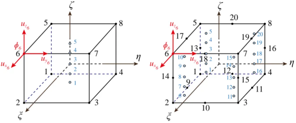
The piezoelectric solid–shell elements SHB8PSE and SHB20E denote an eight-node hexahedral element and a twenty-node one, respectively. These elements have at each of their nodes three displacement degrees of freedom as well as one electric degree of freedom.

designated as the “thickness”, normal to the mean plane of these elements. Also, an in-plane reduced-integration rule is adopted, with 1 n× _int integration points for the SHB8PSE element and 4 n× _int for the SHB20E (see, e.g., Fig. 1, in the particular case of n_int =5).

For the SHB8PSE and SHB20E elements, the spatial coordinates x_i are related to the nodal coordinates x_iI using linear and quadratic shape functions, respectively, as follows:

(

, ,

)

i iI I

x = x N ξ η ζ (5)

where i represents the spatial directions and ranges from 1 to 3; while

I

stands for the node number, which ranges from 1 to 8, for the SHB8PSE element, and from 1 to 20 for the SHB20E. Likewise, the displacement field u_i and potential field

φ

are related to the nodal displacements u_iI and nodal potentials

φ

_I, respectively, using the shape functions

(

)

(

)

, , , , u i iI I I I u u N Nφ ξ η ζ φ φ ξ η ζ  ₌   =  (6)

Note that in Eqs. (5) and (6) above, the convention of implied summation over the repeated index

I

has been adopted.

3.2. Discrete gradient operators

For both elements SHB8PSE and SHB20E, the corresponding discrete gradient operators u

 

B  and _Bφ_ can be derived in the following compact form:

1 ,1 2 ,2 1 ,1 3 ,3 2 ,2 2 ,2 1 ,1 3 ,3 1 ,1 3 ,3 3 ,3 2 ,2 ; T T T T T T T T u T T T T T T T T T T T T T T T T h h h h h h h h h h h h α α α α α α φ α α α α α α α α α α α α α α α α α α  ₊    +   _{ + }  ₊  _{ }   = =_ + _ + +   _{ } +  ₊    +    _{+ +}    0 0 0 0 0 0 B B 0 0 0 b γ b γ b γ b γ b γ b γ b γ b γ b γ b γ b γ b γ (7)

where b , T_j h_{α, j} and γ_αT are detailed in Appendix A. More details can also be found in references [52-55]. Note again that, in Eq. (7) and in what follows, the convention of implied summation over the repeated index

α

is adopted, with

α

ranging from 1 to 4, for the SHB8PSE element, and from 1 to 16 for the SHB20E.

Similar to the purely mechanics-based solid–shell element SHB20 (see, e.g., [55]), the benchmark tests performed with the piezoelectric solid–shell counterpart SHB20E did not reveal any particular locking and, accordingly, no specific enhanced assumed strain

techniques have been applied to this quadratic solid–shell element. By contrast, the original formulation of the linear solid–shell version SHB8PSE has been shown to suffer both from spurious hourglass modes and locking phenomena. Therefore, to circumvent these numerical pathologies, projection of its discrete gradient operator and stabilization of its stiffness matrix are undertaken following the assumed strain method. Note that the projection of the displacement-related discrete gradient operator

B

u is performed in the same way as for the SHB8PS element (see [53]), which leads to a similar form for the stiffness matrix

K

uu. Hence, in the current work, special attention is paid to the impact of the assumed-strain projection on the expressions of the piezoelectric and dielectric matrices

K

uφ and

K

φφ.

3.3. Assumed-strain projection and stabilization of the SHB8PSE

Let us first underline that in Eq. (7), vectors b_i originally defined by Hallquist’s form are replaced by the following mean form proposed by Flanagan and Belytschko [56]:

(

)

, 1 ˆ _{, ,} e u i _V i e dv V

ξ η ζ

=

_∫

b N (8)

Then, using the Hu–Washizu mixed variational principle in conjunction with the assumed strain method proposed by Belytschko and Bindeman [57], the discrete gradient operator Bˆu is projected onto a new operator Bˆu in order to eliminate various types of locking. The latter operator is additively decomposed into two parts, denoted by Bˆ₁₂u and Bˆ₃₄u , as follows:

1 12 34 2 12 34 3 3 12 12 34 2 12 1 12 1 12 3 12 3 12 2 12 ˆ ˆ ˆ ˆ ˆ ˆ ˆ ˆ ˆ ˆ _; ˆ ˆ ˆ ˆ ˆ ˆ ˆ ˆ ˆ ˆ ˆ ˆ ˆ T T T T T T T T T u u T T T T T T T T T T T T  ₊  _{ }   _{ } +   _{ }   _{ } +     _{ }  _{= =}    _{+ +}        _{ }  _{+ +}  _{ }   _{ } + +       0 0 0 0 0 0 0 0 0 0 0 0 B B 0 0 0 0 0 0 0 0 0 0 0 0 b X X b Y Y Z b Z b Y b X b X b Z b Z b Y (9) where , , , ˆ _{ˆ ;} ˆ _{ˆ ;} ˆ _ˆ x y z h h h γ γ γ βγ α α βγ α α βγ α α α β= α β= α β= =

∑

=

∑

=

∑

X γ Y γ Z γ ₍₁₀₎

The stiffness matrix is finally derived as follows:

12

uu uu uu

e = + Stab

K K K (11)

12 12 12 12 34 34 12 34 34 ˆ ˆ ˆ ˆ ˆ ˆ ˆ ˆ e e e e uu u T u V uu u T u u T u u T u Stab _{V V V} dv dv dv dv = ⋅ ⋅ = ⋅ ⋅ + ⋅ ⋅ + ⋅ ⋅

∫

∫

∫

∫

K B C B K B C B B C B B C B (12)

The stabilization stiffness matrix uu Stab

K is computed in a co-rotational coordinate frame. The adopted orthogonal co-rotational coordinate system is defined by the rotation matrix

R

that maps a vector in the global coordinate system to the co-rotational one. The components of the first two column vectors of matrix

R

, denoted a_1i and a_2i, respectively, are given by

(

)

(

)

1 2 1 2 1 2 1,1,1, 1, 1,1,1, 1 1, 1,1,1, 1, 1,1,1 , , 1, 2, 3 with T T T T i i i i a ⋅ a i = − − − − = − − − − = = ⋅ =    Λ Λ ΛΛ ΛΛ Λ Λ Λ ΛΛ Λ Λ ΛΛ Λ x x (13)

Then, the second column vector a₂ is modified in order to make it orthogonal to a₁. To this end, a correction vector a_c is added to a₂ such that:

(

)

1 2 1 2 1 1 1 0 T T c c T ⋅ ⋅ + = ⇒ _{= −} ⋅ a a a a a a a a a (14)

The third base vector a₃ is finally obtained by the cross-product

a

₃

= ∧

a

₁

(

a₂ +a_c

)

, which gives the components of the rotation matrix after normalization by

1 2 3 1 2 3 1 2 3 , , , 1, 2, 3 i i ci i i i i c a a a a R = R = + R = i= + a a a a (15)

For the derivation of the piezoelectric and dielectric matrices

K

uφ and

K

φφ, a similar procedure is followed. As above, the potential-related discrete gradient operator Bˆφ is projected onto Bˆφ, which is then additively decomposed into two parts, denoted by Bˆ₁₂φ and

34 ˆφ B , as follows: 1 12 34 12 2 12 34 34 3 3 12 ˆ ˆ ˆ ˆ ˆ ˆ _; ˆ ˆ ˆ ˆ ˆ T T T T T T T T T φ φ  ₊        = +  =      +   _ _   B B b X X b Y Y Z b Z (16)

Accordingly, the piezoelectric matrix is computed as follows:

12 u u u e Stab φ ₌ φ ₊ φ K K K (17) with

12 12 12 12 34 34 12 34 34 ˆ ˆ ˆ ˆ ˆ ˆ ˆ ˆ e e e e u u T T V u u T T u T T u T T Stab _{V V V} dv dv dv dv φ φ φ φ φ φ = ⋅ ⋅ = ⋅ ⋅ + ⋅ ⋅ + ⋅ ⋅

∫

∫

∫

∫

K B e B K B e B B e B B e B (18)

while the dielectric matrix is given by

12 e Stab φφ ₌ φφ ₊ φφ K K K (19) with 12 12 12 12 34 34 12 34 34 ˆ ˆ ˆ ˆ ˆ ˆ ˆ ˆ e e e e T V T T T Stab V V V dv dv dv dv φφ φ φ φφ φ φ φ φ φ φ = − ⋅ ⋅ = − ⋅ ⋅ − ⋅ ⋅ − ⋅ ⋅

∫

∫

∫

∫

K B B K B B B B B B κκκκ κ κ κ κ κ κ κ κ κ κ κ κ (20)

Note that the stabilization matrices Kuφ_Stab and Kφφ_Stab, related to the piezoelectric and dielectric matrices, are computed in the same co-rotational coordinate frame as that used previously for the computation of the stabilization stiffness matrix. More details can be found in Appendix B.

Moreover, it must be noted that the material properties of the piezoelectric components, which are defined by the elastic, piezoelectric and dielectric permittivity matrices C , e and

κ

, are expressed in a local physical material frame. Hence, to express these matrices in the global coordinate system, an inverse transformation is used, which is defined by a rotation matrix, denoted RRRR. More details on these coordinate system transformations and on the derivation of the associated matrix components are given in Appendix C.

4. Numerical tests and validation

To evaluate the performance of the proposed piezoelectric solid–shell formulations, a selection of representative benchmark tests is conducted in static and vibration analysis, for multilayer beam, plate and shell structures. For all of the simulations, the mesh nomenclature adopted for hexahedral elements is as follows: N

(

₁×N₂×N₃

)

elements, where N₁ denotes the number of elements in the length direction, N₂ is the number of elements in the width direction, and N₃ is the number of elements in the thickness direction. Note that, for the proposed solid–shell elements SHB8PSE and SHB20E, two integration points along the thickness direction are sufficient for the following computations, as the corresponding benchmark tests do not involve material nonlinearities. However, it must be noted that, when nonlinear material behavior models enter into play, more through-thickness integration points are required (for instance, five through-thickness integration points are recommended when elasto-plastic constitutive models are used, see, e.g., reference [53]).

4.1. Static benchmarks

In the case of static analysis, the system of discretized equations (4) reduces to

uu u u φ φ φφ       =             K K K K

φφφφ

U F Q (21)

A set of five benchmark tests taken from the literature is investigated in the following sections. The first and third tests are devoted to beam structures (bimorph and sandwich beam in extension and shear deformation mechanisms, respectively). The second and fourth tests are dedicated to plate structures (investigation of shear locking in thin piezoelectric sensors and shape control of plate with piezoelectric patches, respectively). Finally, the fifth test deals with a piezoelectric sandwich shell structure.

4.1.1. Bimorph pointer

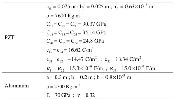
This benchmark test consists of a cantilever beam composed of two layers polarized in two opposite directions (z and –z here). This test has been considered in many works in the literature, among which Tzou and Ye [58], Sze et al. [43] and Klinkel and Wagner [44]. A voltage of ∆ =

φ

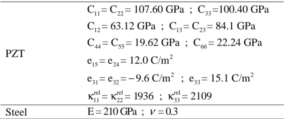
1V is applied on the exterior faces. The geometric dimensions and boundary conditions are reported in Fig. 2.

The material parameters are reported in Table 2, where the results obtained with the proposed piezoelectric solid–shell elements SHB8PSE and SHB20E are compared with those given by their counterparts from ABAQUS, which have the same geometry and the same number of degrees of freedom, namely the three-dimensional linear and quadratic elements C3D8E and C3D20E, respectively. These simulation results are additionally compared to the reference solution given by the following analytical formula:

2 31 2 3 e ( ) 2 z U x x Eh φ ∆ = − (22)

It appears from Table 2 that the proposed piezoelectric solid–shell element SHB8PSE provides a more accurate result than the standard three-dimensional ABAQUS element C3D8E, while requiring much less degrees of freedom. As to the quadratic versions of these elements, the accuracy of the proposed piezoelectric solid–shell element SHB20E is comparable to that of the three-dimensional ABAQUS element C3D20E, while using twice less elements. It is also noteworthy that despite the higher number of elements required for the C3D8E (40 times more elements than the SHB8PSE), its result still exhibits an error of nearly 26% with respect to the reference solution.

In the previous configuration of regular meshes, the higher performance of the proposed solid–shell elements has been clearly shown. In particular, fewer elements are generally required with the proposed solid–shell formulations to achieve convergence, as compared to their ABAQUS counterparts, which allows reducing the computational effort. This superiority

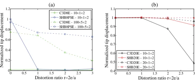
in terms of higher convergence rate is even more evident in presence of distorted meshes. To illustrate this, we consider again the previous piezoelectric bimorph, which is discretized now with distorted meshes as shown in Fig. 3. Two different discretizations are considered for each element, and we investigate the sensitivity of the results to the corresponding distorted meshes. The normalized tip displacement is plotted in Fig. 4 for different values of the distortion parameter r=2 /e a, where a is the in-plane element size and e defines the twist with respect to the regular mesh. For the same mesh discretization of 10x1x2 elements, the results reported in Fig. 4-b show that the relative error for the C3D20E element increases to 50% at a distortion parameter of r=3, when it is only 8% for the SHB20E at the same distortion. Also, with mesh refinement, the relative error decreases to about 5% for the C3D20E element, while it tends to zero for the SHB20E element. Regarding the linear elements, Fig. 4-a reveals that the relative error for the C3D8E element exceeds 20%, at a distortion parameter of r=3, for both of the distorted meshes considered. However, although the SHB8PSE exhibits more sensitivity to mesh distortion than its quadratic counterpart SHB20E, its accuracy is still much better than that of the C3D8E element. This example clearly shows the interest of using solid–shell finite element technology to model piezoelectric structures, which is even more evident in presence of distorted meshes.

4.1.2. Shear locking in thin piezoelectric sensors

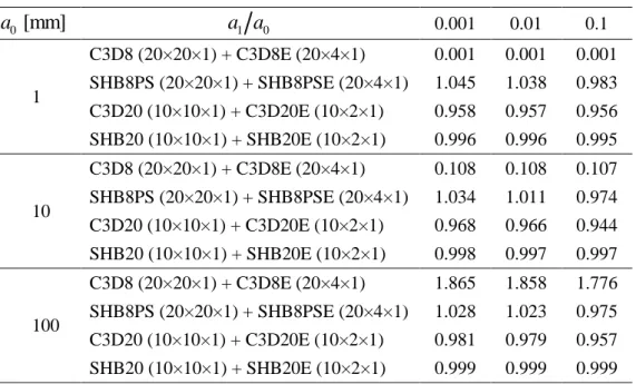
The aim of this benchmark test is to highlight the shear locking phenomenon, which particularly affects linear solid finite elements, when employed to model thin structures. This test has been proposed by Kögl and Bucalem [59], and it is used to assess the effectiveness of the various treatments adopted to prevent such locking phenomena. For this purpose, a square plate of side 1000 mm and thickness a₀ is considered. The plate is clamped at one side and is bent by applying a line force at the opposite edge as shown in Fig. 5. This steel plate is covered by a PZT piezoelectric sensor, which has a width of 200 mm and a thickness

a

₁. The material properties are reported in Table 3. For different configurations of thicknesses, we determine the tip displacement U_zC at point C (see Fig. 5). The reference solution is obtained with a refined mesh using the ABAQUS quadratic element C3D20E.

The results in terms of normalized tip displacements at point C are reported in Table 4 for different plate thicknesses and geometric ratios. It appears that with the SHB8PSE solid–shell element, the relative error is comprised between 1.1% (a₀ =10 mm; a a_{1 0} =0.01) and 4.5% (a₀ =1 mm; a a_{1 0} =0.001). By contrast, using the same mesh of 20×4×1 hexahedral elements, the C3D8E element exhibits very poor results due to its high sensitivity to locking effects. Moreover, the C3D8E shows high sensitivity to the element aspect ratio, as it provides results that are 1000 times underestimated, for a0=1 mm, to almost 2 times overestimated, for

0=100 mm

a . Therefore, to achieve better results with the C3D8E element, much more refined meshes would be required, thereby significantly increasing the CPU time.

This benchmark test also demonstrates the effectiveness of the assumed-strain projection technique applied to the piezoelectric solid–shell element SHB8PSE to prevent various locking phenomena.

4.1.3. Extension and shear piezoelectric actuation mechanisms

In this third benchmark test, we consider two configurations of cantilever sandwich beams, as illustrated in Fig. 6, which are actuatable in extension (a) and in shear (b), respectively. These tests represent excellent benchmark problems for their selectivity, and have become popular, as commonly studied in a number of literature works, including those of Zhang and Sun [60, 61] and Benjeddou et al. [62].

The materials are polarized in the z-direction for the extension mechanism, and in the x-direction for the shear mechanism. In order to bend the beam, voltages are applied to the upper and lower surfaces of the piezoelectric layers, inducing electric bending forces. Thus, for the shear actuation mechanism, a voltage of ∆ =

φ

20V is applied to the piezoelectric core, while for the extension actuation mechanism, voltages of ∆ = ±

φ

10V are applied to the surface of the actuators. The corresponding material properties are all reported in Table 5. The numerical results obtained with the proposed SHB8PSE and SHB20E piezoelectric solid– shell elements are compared, on the one hand, with those taken from the literature [60-62] and, on the other hand, with those given by state-of-the-art ABAQUS elements that have equivalent geometry and kinematics, namely the C3D8E and C3D20E piezoelectric solid elements.

Two cases with regard to the piezoelectric layer arrangement are considered. The first case corresponds to the situation when the piezoelectric layers cover the entire length of the beam; while in the second case, the position of the actuator varies in the 10-90 mm range. We start by analyzing the first case, and the corresponding simulation results are reported in Fig. 7. Note that, in this first case and for the shear actuation mechanism, there is no rigid foam and, instead, the piezoelectric actuator covers the entire core layer. It appears from Fig. 7 that the results obtained with the proposed SHB8PSE and SHB20E elements are in excellent agreement with those given by ABAQUS elements, while systematically requiring a fewer number of elements to achieve convergence. However, the literature results, which are obtained by 2D modeling, seem to overestimate the transverse deflection in the case when the beam is actuated by piezoelectric expansion (see Fig. 7-a).

In the second case, where the actuator position varies in the 10-90 mm range, the deflection at the free edge is investigated for each position of the piezoelectric patches. Here again, the simulation results are compared with those taken from the literature (Benjeddou et al. [62] and Piefort [63], where only shear mechanism results are available) as well as with those given by the ABAQUS linear and quadratic piezoelectric solid elements C3D8E and C3D20E. From Fig. 8, it is observed that the results obtained with the SHB8PSE and SHB20E elements are in good agreement with those of the literature as well as with those yielded by ABAQUS elements, for both actuation mechanisms. However, it is worth noting that the results obtained with the proposed solid–shell elements converge faster than those of existing

conventional elements (i.e., relatively fewer elements are required with the SHB8PSE and SHB20E formulations to achieve convergence, as shown in Fig. 8).

4.1.4. Square plate with piezoelectric patch models

One important advantage taken from the piezoelectric behavior is in the application to the shape control of structures. In order to show the interest of solid–shell finite elements in this type of modeling, we consider a square aluminum plate of 200×200 mm2 with a thickness of 8 mm. This plate is covered on both sides with four pairs of localized PZT-5H patches in various configurations, as shown in Fig. 9. Each patch has dimensions of 40×40 mm2 with a thickness of 1 mm. The objective of this test is to investigate the optimal location of piezoelectric patches for shape control. With regard to loading conditions, the plate is subjected to a uniformly distributed load of 100 N.m−2 over its entire surface. A constant voltage is then supplied incrementally to the piezoceramic actuators, which are polarized in opposite directions, until the plate is flattened. Fig. 10 shows the centerline deflection of the composite plate along the x-direction under different input voltages. The results provided by the solid–shell elements SHB8PSE and SHB20E are compared with those given by the ABAQUS solid elements C3D8E and C3D20E. On the whole, it appears that fewer overall degrees of freedom are required for the proposed solid–shell elements to achieve convergence, as compared to ABAQUS elements. It is also noteworthy that despite the high number of overall degrees of freedom required by the C3D8E element, it provides less accurate results than the SHB8PSE, especially in configuration (c), where the error margin reaches 16%.

In addition, the analysis of the plots in Fig. 10 shows that the (a) and (d) configurations are more effective in terms of shape control (plate flatness recovery). Note however that configuration (a) requires up to −20 V by pair of patches to recover the initial shape of the plate, whereas only 2 V are sufficient for configuration (d).

4.1.5. Shallow cylindrical sandwich blade

In order to assess the capabilities of the proposed solid–shell elements in geometric nonlinear analysis, a cantilever shallow cylindrical sandwich shell with 300 mm for both of its straight and curved edges, as depicted in Fig. 11, is considered. A similar model has been proposed by Kioua and Mirza [64], but no comparison with available finite element technologies was attempted. Here again, the host shell is made in aluminum and has a thickness of 2.50 mm. This shell is entirely covered on both sides with a thin PZT-5H layer of 0.25 mm thickness polarized across the thickness. A voltage of 50 V is applied to each piezoelectric layer (the internal faces are connected to ground, while 50 V is applied to the external faces) to induce bending actuation. Three values for the ratio are considered ( ). The considered layup configuration for the laminated shell causes high stiffness coupling and, consequently, also generates a twisting deformation. The deflections along paths A, B and C, as shown in Fig. 11, are investigated.

R b

{

1, 10,

}

R b= ∞

In Fig. 12, the results provided by the solid–shell finite elements SHB8PSE and SHB20E are compared to those given by the ABAQUS solid elements C3D8E and C3D20E. Once again, the good behavior of the SHB8PSE and SHB20E elements is clearly observed, which highlights the benefit of using the proposed solid–shell elements in this kind of analysis.

With this preliminary set of static tests performed, focus is placed in the following sections on free vibration modeling of sandwich structures that contain piezoelectric layers, in order to evaluate the performance of the proposed solid–shell formulations.

4.2. Vibration test problems

In the case of free vibration analysis, the system of discretized equations (4) becomes

2 uu u uu u φ φ φφ

ω

        − =         _{       }   0 K K M 0 0 K K 0 0 U

φφφφ

(23)

In the following sections, a set of free vibration tests both in open-circuit and short-circuit configurations will be carried out on beam, plate and shell structures.

4.2.1. Beam benchmark tests

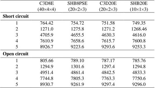
We consider here two sandwich beam models. These benchmark tests are similar to those previously presented in static analysis with shear and extension actuation mechanisms; however, they have different geometric parameters, as shown in Fig. 13. The elastic layers are made of aluminum, while the piezoelectric layers are made in PZT-5H material. The modal analysis is performed using both the short-circuit (SC) and open-circuit (OC) configurations. In Tables 6 and 7, the first five free vibration frequencies are provided, revealing that the results obtained with the SHB8PSE and SHB20E elements are in good agreement with those given by the ABAQUS quadratic solid element C3D20E. It should be emphasized, however, that less overall degrees of freedom are required with the proposed solid–shell elements to achieve accurate results, as compared to their ABAQUS solid element counterparts. It is also worth noting that, despite the higher number of overall degrees of freedom required by the C3D8E element, its results still fall far from the reference solutions, especially for high frequencies.

4.2.2. Sandwich plate

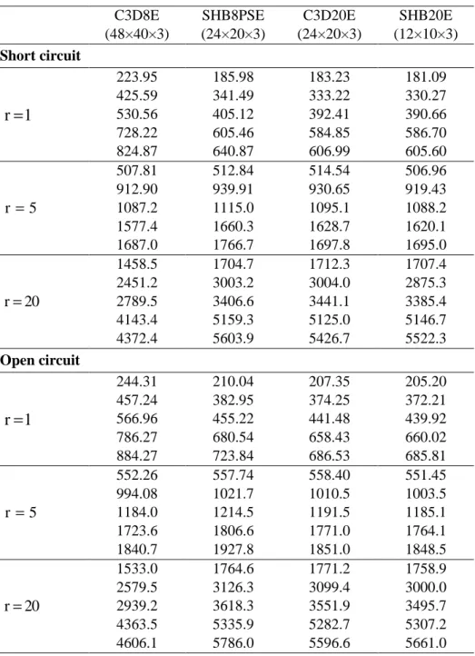
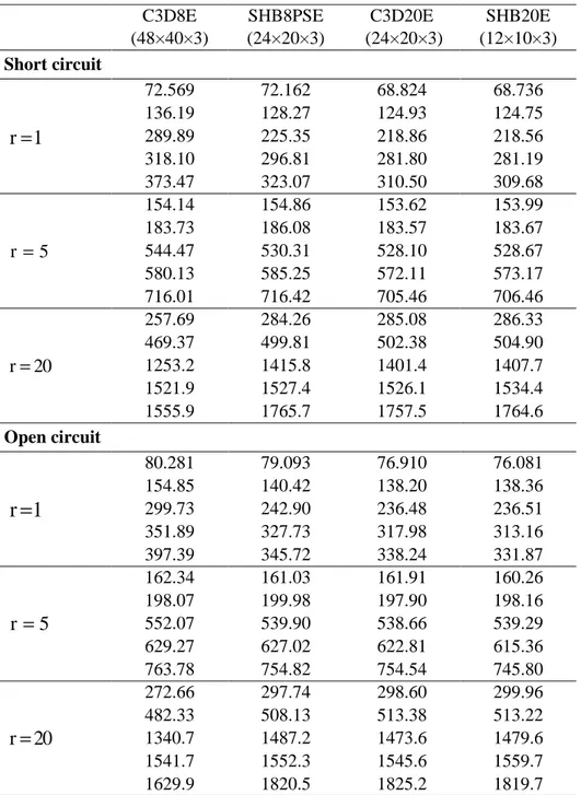
In this second example of this category of benchmark problems, we investigate the free vibration response of a simply supported sandwich plate. The plate consists of two piezoelectric faces, in PZT-5H material polarized along the thickness, covering a core made of aluminum with a varying thickness. The piezoelectric faces have a thickness of 1 mm, while the other geometric dimensions are shown in Fig. 14. Different thicknesses for the aluminum core are considered, according to a geometric ratio r , in order to analyze the sensitivity to thickness reduction of the results given by the proposed solid–shell elements.

The first five free vibration frequencies are investigated in both short-circuit and open-circuit configurations and are reported in Table 8.

According to Table 8, the results obtained with the solid–shell finite elements SHB8PSE and SHB20E are in good agreement with those of the reference ABAQUS element C3D20E. It should be noted, however, that fewer degrees of freedom are required for the proposed solid–shell elements, as compared to their counterparts with the same kinematics. Note also that, despite the finer mesh required by the C3D8E element, its results fall most of the time far from the reference solutions.

4.2.3. Cantilever plate with piezo-patches

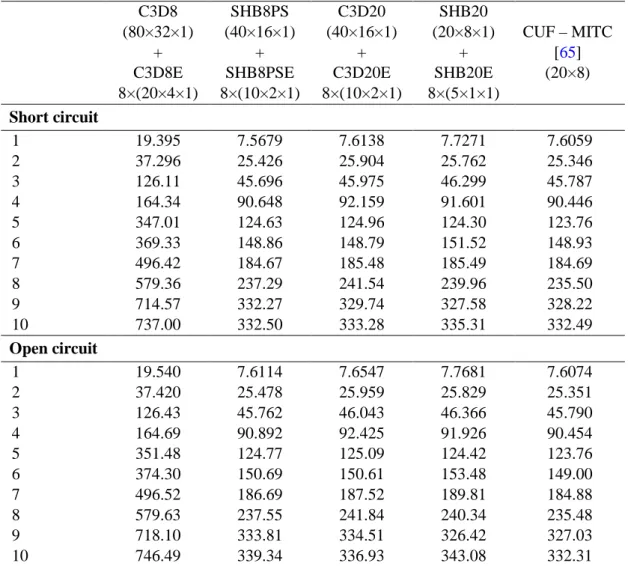
This benchmark test has been proposed by Cinefra et al. [65] and concerns the free vibration analysis of a cantilever aluminum plate with four pairs of piezoelectric patches. More specifically, four patches are bonded on the top surface, with the four others symmetrically bonded on the bottom surface (see Fig. 15). The material and geometric properties of the structure are reported in Table 9. The first ten free vibration frequencies are investigated in both short-circuit and open-circuit configurations and are reported in Table 10. The results obtained with the proposed solid–shell elements are compared to those yielded by ABAQUS elements and also to those given in Cinefra et al. [65]. The latter are based on a model derived from the CUF with finite element discretization employing the 9-node MITC element (Mixed Interpolation of Tensorial Components). The analysis in Table 10 shows that the results obtained with the proposed solid–shell elements are in good agreement with those of the reference element C3D20E as well as with those given by the CUF-MITC model [65]. It also clearly appears that the linear ABAQUS solid element C3D8E, despite the high number of overall degrees of freedom, provides very poor results due to its high sensitivity to locking effects.

In the following sections, free vibration analysis of shell structures provided with piezoelectric materials will be conducted. The aim is to assess the performance and reliability of the proposed solid–shell elements in the modeling of sandwich structures involving geometric nonlinearities. In this latter context, two benchmark tests will be analyzed.

4.2.4. Curved cantilever sandwich blade

In this test problem, a curved cantilever sandwich blade is considered. A similar test has been investigated by Zouari et al. [66], based on the experimentations conducted by Olson and Lindberg [67], but only involved purely elastic behavior. Here, similar to the previously studied test, the core is made of aluminum, while the faces are made in PZT-5H material, as shown in Fig. 16. Several core thicknesses are also investigated both in short-circuit and open-circuit configurations. From the results reported in Table 11, it appears that, once again, the conventional solid finite elements C3D8E and C3D20E require finer meshes to provide accurate results, as compared to the proposed solid–shell formulations. One may also notice

exhibits a margin of error that exceeds 20%, for the fifth frequency and r = 1, while the relative error with the SHB8PSE is of about 4% only.

4.2.5. Hemispherical sandwich shell with a hole

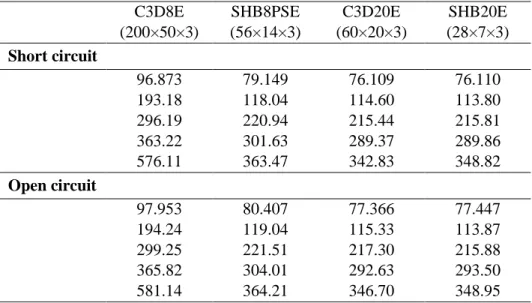
The last benchmark test in this category is concerned with a doubly curved sandwich shell structure. This consists of a hemispherical shell, with an 18° hole and a mean radius of 200 mm, as depicted in Fig. 17. The host structure is made of aluminum material and has a thickness of 1.50 mm. This hemispherical shell is entirely covered on both sides with a thin PZT-5H layer, which is polarized across its thickness of 0.25 mm. The shell structure is clamped over the entire holed face. The current analysis consists in investigating the first five modes in both short-circuit and open-circuit configurations, which are illustrated in Fig. 18. The results in terms of the corresponding natural frequencies (first five natural frequencies) are summarized in Table 12.

As previously done, the results obtained with the proposed solid–shell formulations are compared in Table 12 with their ABAQUS counterparts, which are based on the same geometry and kinematics. From Table 12, it appears that, while using coarser meshes, the results provided by the developed solid–shell elements are in good agreement with the reference solution given by the C3D20E ABAQUS quadratic piezoelectric element. Again, the worst results are by far those provided by the C3D8E ABAQUS solid element, which is attributable to its high sensitivity to locking effects.

5. Summary and conclusions

In the current contribution, two new hexahedral piezoelectric solid–shell finite elements have been developed. These finite element technologies consist of an eight-node hexahedron, denoted as SHB8PSE, and a twenty-node hexahedron, designated as SHB20E. These formulations are based on purely three-dimensional kinematics and, accordingly, the resulting finite elements have at each of their nodes three translational degrees of freedom and one electric degree of freedom. To provide these elements with some desirable shell features, and to alleviate locking effects, an in-plane reduced-integration scheme is adopted, with a user-defined number of integration points along the thickness direction. The constitutive law is also expressed in a local physical coordinate system, which is attached to the element mid-plane, in order to enhance immunity with regard to thickness locking.

Particular attention has been paid to the polarization of piezoelectric patches, which plays a very important role in the mechanism of deformation. Both static and free vibration benchmark tests have been successfully conducted on structures ranging from simple beams and plates to more complex sandwich shells. The simulation results obtained with the newly devised solid–shell elements have been compared with reference solutions taken from the literature and also with state-of-the-art finite elements available in ABAQUS. Among the latter, the quadratic hexahedral piezoelectric solid element C3D20E is often taken as reference. In all of the benchmark tests investigated, the solid–shell elements SHB8PSE and

SHB20E have shown better performance, as compared to their ABAQUS counterparts, the C3D8E and C3D20E, respectively, while systematically necessitating a fewer number of elements for similar accuracy. Also, although in some situations of severe nonlinearities the SHB8PSE element may exhibit some over-stiffness due to locking, its accuracy and convergence rate remain overall much better than those of the C3D8E element. In future work, it would be interesting to further improve the performance of the SHB8PSE element, by using for instance other advanced enhanced assumed strain methods. It would be also interesting to extend this study to the modeling of vibration control of multilayer structures with piezoelectric materials in complete layers or patches.

Appendix A. Derivation of the discrete gradient operators

For the SHB8PSE solid–shell element, the combination of Eqs. (5) and (6), along with the expression of the shape functions for linear eight-node elements, allows expanding the displacement field in the following form:

0 1 1 2 2 3 3 1 1 2 2 3 3 4 4 1 , 2 , 3 , 4 i i i i i i i i i u a a x a x a x c h c h c h c h h ηζ h ξζ h ξη h ξηζ = + + + + + + +   = = = =  (A.1)

By evaluating equation (A.1) at the nodes of the element, one can obtain a set of eight-equation systems defined by

0 1 1 2 2 3 3 1 1 2 2 3 3 4 4

1, 2,3

i

a

i

a

i

a

i

a

i

c

i

c

i

c

i

c

i

i

=

+

+

+

+

+

+

+

=

d

s

x

x

x

h

h

h

h

(A.2)

where

d

_i and

x

_i denote the nodal displacements and nodal coordinates, respectively, while vectors s and

h

_α are defined by

(

)

(

)

(

)

(

)

(

)

1 2 3 4 1, 1, 1, 1, 1, 1, 1, 1 1, 1, 1, 1, 1, 1, 1, 1 1, 1, 1, 1, 1, 1, 1, 1 1, 1, 1, 1, 1, 1, 1, 1 1, 1, 1, 1, 1, 1, 1, 1 T T T T T = = = = − − − − − − − − − − − − − − − −  ₌         s h h h h (A.3)

To determine the yet unknown constants

a

_ji and c_αi, the derivatives of the shape functions evaluated at the origin of the reference frame are introduced

, 0 ( ) 1, 2, 3 i i i i x _{ξ η ζ= = =} = =∂ = ∂ 0 N b N _(A.4)

Finally, using a set of preliminarily established orthogonality relations, one obtains

(

)

3 1 ; 1 where , =1,...,4 8 T T ji j i i i T j j j a c_{α α} α α α

α

= = ⋅ = ⋅   =  − ⋅  

∑



γγγγ

γγγγ

b d d h h x b (A.5)

In the case of the SHB20E solid–shell element, combining Eqs. (5) and (6), in conjunction with the explicit form of the shape functions for quadratic twenty-node elements, leads to the following expansion for the displacement field:

0 1 1 2 2 3 3 1 1 2 2 3 3 4 4 5 5 6 6 7 7 8 8 9 9 10 10 11 11 12 12 13 13 14 14 15 15 16 16 2 2 2 1 2 3 4 5 6 7 + + + + + + , , , , , , , i i i i i i i i i i i i i i i i i i i i i u a a x a x a x c h c h c h c h c h c h c h c h c h c h c h c h c h c h c h c h h h h h h h h h ξζ ηζ ξη ξ η ζ ξηζ = + + + + + + + + + + + + + = = = = = = = 2 2 2 2 2 2 8 9 10 11 12 13 2 2 2 14 15 16 , , , , , , , , h h h h h h h h ξ η ξ ζ η ξ η ζ ζ ξ ζ η ξ ηζ ξη ζ ξηζ         _{= = = = = =}   = = =  (A.6)

Similarly, the evaluation of equation (A.6) at the nodes of the element leads to three systems of 20 equations defined by 0 1 1 2 2 3 3 1 1 2 2 3 3 16 16

1, 2,3

i

a

i

a

i

a

i

a

i

c

i

c

i

c

i

c

i

i

⋯

d

=

s

+

x

+

x

+

x

+

h

+

h

+

h

+

+

h

=

(A.7)

where d_i and x_i represent the nodal displacements and nodal coordinates, respectively, while vectors s and h_α are defined by

(

)

(

)

(

)

1 2 3 1, 1, 1, 1, 1, 1, 1, 1, 1, 1, 1, 1, 1, 1, 1, 1, 1, 1, 1, 1 1, 1, 1, 1, 1, 1, 1, 1, 0, 1, 0, 1, 0, 0, 0, 0, 0, 1, 0, 1 1, 1, 1, 1, 1, 1, 1, 1, 1, 0, 1, 0, 0, 0, 0, 0, 1, 0, 1, 0 1, 1, 1, 1, T T T T − − − − − − − − − − − − − − s h h h = = = =

(

)

(

)

(

)

4 5 6 1, 1, 1, 1, 0, 0, 0, 0, 1, 1, 1, 1, 0, 0, 0, 0 1, 1, 1, 1, 1, 1, 1, 1, 0, 1, 0, 1, 1, 1, 1, 1, 0, 1, 0, 1 1, 1, 1, 1, 1, 1, 1, 1, 1, 0, 1, 0, 1, 1, 1, 1, 1, 0, 1, 0 1, 1, 1, 1, 1, 1, 1, 1, 1 T T T − − − − h h h = = =

(

)

(

)

(

)

7 8 9 , 1, 1, 1, 0, 0, 0, 0, 1, 1, 1, 1 1, 1, 1, 1, 1, 1, 1, 1, 0, 0, 0, 0, 0, 0, 0, 0, 0, 0, 0, 0 1, 1, 1, 1, 1, 1, 1, 1, 0, 0, 0, 0, 1, 1, 1, 1, 0, 0, 0, 0 1, 1, 1, 1, 1, 1, 1, 1, 0, 1, 0, 1, T T T − − − − − − − − − − − − − − − − h h h = = =

(

)

(

)

(

)

10 11 12 0, 0, 0, 0, 0, 1, 0, 1 1, 1, 1, 1, 1, 1, 1, 1, 0, 0, 0, 0, 1, 1, 1, 1, 0, 0, 0, 0 1, 1, 1, 1, 1, 1, 1, 1, 1, 0, 1, 0, 0, 0, 0, 0, 1, 0, 1, 0 1, 1, 1, 1, 1, 1, 1, 1, 0, 1, 0, 1, 0, 0, 0, T T T − − − − − − − − − − − − − − − − − h h h = = =

(

)

(

)

(

)

13 14 15 0, 0, 1, 0, 1 1, 1, 1, 1, 1, 1, 1, 1, 1, 0, 1, 0, 0, 0, 0, 0, 1, 0, 1, 0 1, 1, 1, 1, 1, 1, 1, 1, 0, 0, 0, 0, 0, 0, 0, 0, 0, 0, 0, 0 1, 1, 1, 1, 1, 1, 1, 1, 0, 0, 0, 0, 0, 0, 0, 0, 0, 0, T T T − − − − − − − − − − − − − − − h h h = = =

(

)

(

)

16 0, 0 1, 1, 1, 1, 1, 1, 1, 1, 0, 0, 0, 0, 0, 0, 0, 0, 0, 0, 0, 0 T − − − − h                               ₌  (A.8)

In a similar way, using some preliminarily established orthogonality conditions, it can be shown that the yet unknown constants

a

ji and cαi are given by the same Eq. (A.5). However, the previous expressions of vectors

γγγγ

_α must be replaced here by

(

)

(

)

(

(

)

)

(

(

)

)

1 1 1 2 2 2 3 3 3 4 4 4 5 5 5 6 6 4 4 4 4 5 5 5 5 4 5 T T T j j j j j j T T T T j j j j n n n n n n α α α α α α α γγγγ h h x b h h x b h h x b h s h s x b h s h s x b h s = − ⋅ + − ⋅ + − ⋅ _ _{ }_ _ _  _ _{ } _ _{ }      + _ − _−__ − _⋅ __{ }+ __ − _−__ − _⋅ _ _          _  + _ − 

(

(

)

)

(

)

(

)

(

(

)

)

(

(

)

)

(

)

(

)

(

(

)

)

(

(

)

)

(

)

6 7 7 7 8 8 8 9 9 9 10 10 10 11 11 11 12 12 12 13 13 13 14 14 14 4 5 T T T j j j j T T T j j j j j j T T T j j j j j j T j n n n n n n n n α α α α α α α α h s x b h h x b h h x b h h x b h h x b h h x b h h x b h h x b h h x  _ _ _    _{− − ⋅ } _{+ − ⋅ ⋅}      _{ } _    + − ⋅ ⋅ + − ⋅ ⋅ + − ⋅ ⋅ + − ⋅ ⋅ + − ⋅ ⋅ + − ⋅ ⋅ +

(

− ⋅

)

15

(

15

(

15

)

)

16

(

16

(

16

)

)

T T j nα j j nα j j b h h x b h h x b ⋅ + − ⋅ ⋅ + − ⋅ ⋅ (A.9)

1 1 0 0 0 0 0 0 0 0 0 0 0 0 0 0 4 4 1 1 0 0 0 0 0 0 0 0 0 0 0 0 0 0 4 4 1 1 0 0 0 0 0 0 0 0 0 0 0 0 0 0 4 4 3 1 1 0 0 0 0 0 0 0 0 0 0 0 0 0 8 8 8 1 3 1 0 0 0 0 0 0 0 0 0 0 0 0 0 8 8 8 1 1 3 0 0 0 0 0 0 0 0 0 0 0 0 0 8 8 8 1 0 0 0 0 0 0 0 0 0 0 0 0 0 0 0 8 3 1 0 0 0 0 0 0 0 0 0 0 0 0 0 0 20 10 3 1 0 0 0 0 0 0 0 0 0 0 0 0 0 0 20 10 3 1 0 0 0 0 0 0 0 0 0 0 20 10 n_αβ − − − − = − −       0 0 0 0 1 3 0 0 0 0 0 0 0 0 0 0 0 0 0 0 10 20 1 3 0 0 0 0 0 0 0 0 0 0 0 0 0 0 10 20 1 3 0 0 0 0 0 0 0 0 0 0 0 0 0 0 10 20 1 1 0 0 0 0 0 0 0 0 0 0 0 0 0 0 4 8 1 1 0 0 0 0 0 0 0 0 0 0 0 0 0 0 4 8 1 1 0 0 0 0 0 0 0 0 0 0 0 0 0 0 4 8 − − − − − −                                                                                                            (A.10)

Appendix B. Computation of the stabilization matrices for the SHB8PSE

As mentioned before, the stabilization matrices for the SHB8PSE element are computed in a co-rotational coordinate frame before being transformed to the orthotropy frame of the piezoelectric material. In this orthogonal co-rotational coordinate frame, which has been previously defined by a rotation matrix R given by Eqs. (13)-(15), several terms of the stabilization matrices are shown to simplify. Indeed, because this system of co-rotational coordinates is chosen to be aligned with the reference frame, the relationships between the two coordinate systems can be approximated by

1 1 8 0 ; T i i i i i i j i j i x x x i j x ξ ξ ξ ξ ∂  = = ⋅ _{∂ ∂ ∂}   _∂ ∂  _{= = ≠} _{∂ ∂}  ɶ ɶ ɶ ɶ ɶ Λ ΛΛ Λ x (B.1)

where vector

ɶx

_i refers to the nodal coordinates expressed in the co-rotational frame, and repeated indices here do not indicate a summation rule. Then, using Eq. (B.1), the following simplifications are demonstrated (see [53] for more details):

3 3 1 1 2 2 , , 4,

8

8

0,

,

,

8

8

8

T T T j k i k i i j i T i T i i i i i

h

h

h

h

J

x

ξ ξ

ξ

∂

⋅

⋅

⋅

=

=

=

=

=

∂

⋅

⋅

ɶ

ɶ

ɶ

ɶ

ɶ

ɶ

ɶ

Λ

ΛΛ

Λ

Λ

Λ

Λ

Λ

Λ

Λ

Λ

Λ

Λ

Λ

Λ

Λ

Λ

Λ

Λ

Λ

x

x

x

x

x

(B.2)

where Jɶ denotes the determinant of the Jacobian matrix. Note again that the repeated indices in Eq. (B.2) do not indicate a summation rule. In addition, the indices i, j and k are pairwise distinct and take values 1, 2 and 3, with all of the possible permutations. Finally, Eq. (B.2) leads to the following expressions:

, 2 2 2 , , 4, , , 0 ( )( ) 1 ( ) ( ) 3 ( ) 3 ( ) 1 ( ) 3 e e e e e i j V T T j j k k ii _V j i _V k i _V i T i i T ij i j j i k k V h dv H h dv h dv h dv H h h dv =  _{⋅ ⋅} = = = =   _⋅   = = ⋅ 

∫

∫

∫

∫

∫

ɶ ɶ ɶ ɶ Λ Λ Λ Λ Λ Λ Λ Λ Λ ΛΛ Λ Λ ΛΛ Λ x x x x (B.3)

By replacing the expressions (B.3) in Eq. (12), providing the stabilization stiffness matrix, one obtains 11 12 13 21 22 23 31 32 33 uu Stab     =_{ }     k k k K k k k k k k (B.4)

where the 8×8 matrices k_ij are given by

11 11 3 3 4 4 22 22 3 3 4 4 33 11 4 4 1 ˆ ˆ ˆ ˆ ( 2 ) 3 1 ˆ ˆ ˆ ˆ ( 2 ) 3 1 ˆ ˆ ( 2 ) 3 , T T T T T ij H H H i j

λ

µ

λ

µ

λ

µ

 _{= +}  ₊   _ _   _{ } = + +  _{ }      _{= +}   _{= ≠}  k k k k 0

γ γ

γ γ

γ γ

γ γ

γ γ

γ γ

γ γ

γ γ

γ γ

γ γ

γ γ

γ γ

γ γ

γ γ

γ γ

γ γ

γ γ

γ γ

γ γ

γ γ

(B.5)

where

λ

=E

ν

/(1−

ν

2) and

µ

=E/ 2(1+

ν

), with E being the Young modulus and

ν

the Poisson ratio.

Similarly, the stabilization matrices Kuφ_Stab and Kφφ_Stab, related to the piezoelectric and dielectric matrices, are obtained as

11 31 11 3 3 4 4 11 21 21 32 22 3 3 4 4 31 31 11 11 31 11 3 3 4 4 1 ˆ ˆ ˆ ˆ 3 1 ˆ ˆ ˆ ˆ ; 3 1 ˆ ˆ ˆ ˆ ; 3 u T T u u u u T T Stab u u T T Stab e H e H H φ φ φ φ φ φ φ φφ φφ φφ _κ    = +  _ _         =_{ }  = _ + _        _{ =}       = −_{ } = _ + _   k k K k k k k 0 K k k γ γ γ γ γ γ γ γ γ γ γ γ γ γ γ γ γ γ γ γ γ γ γ γ γ γ γ γ γ γ γ γ γ γ γ γ γ γγ γ γ γγ γ γ γ γ γ (B.6)

Appendix C. Transformation of tensors from local (material) frame to global frame

The piezoelectric properties of the materials are specified in a local orthotropy frame inherent to the material. For the computation of the different matrices involved (e.g., stiffness, piezoelectric and dielectric permittivity matrices), it is necessary to evaluate these properties in a global fixed coordinate system. For this purpose, a rotation matrix RRRR _{is used for the}

transformation of vector and matrix components from the global frame to the local physical frame. Hence, the components

C

_ijkl,

e

_ijk and

κ

_ij of the tensors C , e and

κκκκ

, expressed in the global coordinate system, are related to their components ˆC_mnop, ˆe_mno and κˆ_mn in the local material frame by the following relationships:

ˆ C ˆ e e ˆ Cijkl im jn ko lp mnop ijk im jn ko mno ij im jn mn  ₌  =   κ = κ  R R R R R R R R R (C.1)

In matrix form, Eq. (C.1) can be rewritten as

ˆ ˆ ˆ T T T  _{= ⋅ ⋅}  = ⋅ ⋅   = ⋅ ⋅  C C e e T T T κ κ κ κ κ κ κ κ R R R R R R RR RR R R (C.2) where