On the properties of turbulent boundary layer over polar cusps

HAL Id: hal-00331062

https://hal.archives-ouvertes.fr/hal-00331062

Submitted on 1 Jan 2002

HAL is a multi-disciplinary open access

archive for the deposit and dissemination of

sci-entific research documents, whether they are

pub-lished or not. The documents may come from

teaching and research institutions in France or

abroad, or from public or private research centers.

L’archive ouverte pluridisciplinaire HAL, est

destinée au dépôt et à la diffusion de documents

scientifiques de niveau recherche, publiés ou non,

émanant des établissements d’enseignement et de

recherche français ou étrangers, des laboratoires

publics ou privés.

On the properties of turbulent boundary layer over

polar cusps

S. Savin, J. Büchner, G. Consolini, B. Nikutowski, L. Zelenyi, E. Amata, H.

U. Auster, J. Blecki, E. Dubinin, K. H. Fornacon, et al.

To cite this version:

S. Savin, J. Büchner, G. Consolini, B. Nikutowski, L. Zelenyi, et al.. On the properties of turbulent

boundary layer over polar cusps. Nonlinear Processes in Geophysics, European Geosciences Union

(EGU), 2002, 9 (5/6), pp.443-451. �hal-00331062�

Nonlinear Processes

in Geophysics

c

European Geosciences Union 2002

On the properties of turbulent boundary layer over polar cusps

1_{Space Research Institute, Russian Academy of Sciences, Profsoyuznaya 84/32, Moscow, 117810, Russia} 2_{Interplanetary Space Phys. Inst., CNR, Roma, Italy}

3_{Max-Planck-Institut f¨ur Aeronomie, Katlenburg-Lindau, Germany} 4_{Space Res. Center, Polish Academy Sci., Warsaw, Poland}

5_{Laboratory Phys. and Chemistry Environment, Orleans, France} 6_{University of Massachusetts at Lowell, Lowell, MA, USA} 7_{CESR, Toulouse, France}

8_{Charles University, Prague, Czech Republic} 9_{University of Oslo, Norway}

10_{Kyushu University, Japan}

11_{Technical University, Braunschweig, Germany}

Received: 5 January 2002 – Accepted: 8 February 2002

Abstract. We study properties of nonlinear magnetic

fluctu-ations in the turbulent boundary layer (TBL) over polar cusps during a typical TBL crossing on 19 June 1998. Interball-1 data in the summer TBL are compared with that of Geotail in solar wind (SW) and Polar in the northern TBL. In the TBL two characteristic slopes are seen: ∼ − 1 at (0.004– 0.08) Hz and ∼ − 2.2 at (0.08–2) Hz. We present evidences that random current sheets with features of coherent solitons can result in: (i) slopes of ∼ − 1 in the magnetic power spec-tra; (ii) demagnetization of the SW plasma in “diamagnetic bubbles”; (iii) nonlinear, presumably, 3-wave phase coupling with cascade features; (iiii) departure from the Gaussian statistics. We discuss the above TBL properties in terms of intermittency and self-organization of nonlinear systems, and compare them with kinetic simulations of reconnected cur-rent sheet at the nonlinear state. Virtual satellite data in the model current sheet reproduce valuable cascade-like spectral and bi-spectral properties of the TBL turbulence.

1 Introduction

The paper is devoted to the experimental study of the singu-lar regions at high-latitude magnetopause, where the magne-tosheath (MSH) flow interaction with the exterior cusp re-sults in the creation of the turbulent boundary layer (TBL). In the TBL magnetic fluctuations are of the order of the DC magnetic field, and their power reaches 10–30% of the thermal ion density (Savin et al., 1998a, b, 2001). Early

Correspondence to: S. Savin (ssavin@iki.rssi.ru)

single spacecraft observations with Heos-2 and later with Prognoz-7, 8, 10 have shown that the magnetopause (MP) position and MSH plasma flow structures are quite vari-able near the cusp, a magnetospheric region that is crucial for magnetosheath plasma entry (Haerendel and Paschmann, 1975; Klimov et al., 1986; Lundin et al., 1991). For a syn-opsis of measurements and models of the low altitude cusp, the reader is referred to the review by Smith and Lockwood (1996). Here we identify the MP as the innermost current sheet where the magnetic field turns from Earth-controlled to magnetosheath-controlled (Haerendel and Paschmann, 1975).

At the cusp the magnetopause is indented. The indentation was first predicted by Spreiter and Briggs (1962) and then de-tected by HEOS-2 (Paschmann et al., 1976), ISEE (Petrinec and Russell, 1995), and Hawkeye-1 (Chen et al., 1997). The plasma in the vicinity of this indentation is highly disturbed and/or stagnant MSH plasma. The TBL is a sub-region of the MSH/cusp interface with nonlinear magnetic perturba-tions. It is located just outside and/or at the near-cusp mag-netopause and has been found recently to be a permanent feature (Savin et al., 1998b, 2001, 2002a, b; Klimov et al., 1986). Here the energy density of the ultra low-frequency (ULF) magnetic fluctuations is comparable to the ion kinetic, thermal, and DC magnetic field densities. The ULF power is usually several times larger than that in the MSH, and one or two orders of magnitude larger than that inside the mag-netopause. Haerendel (1978) was the first one to introduce the turbulent boundary layer in cusp physics in a discussion on the interaction of the magnetosheath (MSH) flow with

444 S. Savin et al.: On the properties of turbulent boundary layer over polar cusps

the magnetopause at the flank of the tail lobe. In Savin et al. (2002a), the reader can find a review of the previous TBL studies and of the respective instrumentation.

This paper deals with the TBL during negative dominant By IMF conditions. In such a configuration the boundary layer is developed at high latitudes (Fedorov et al., 2000; Maynard et al., 2001). We discuss spectral and statistical properties of the turbulence at the cusp/MSH interface on the basis of the data from Interball-1 on 19 June 1998, when Interball-1 and Polar crossed the southern and northern TBLs (i.e. winter and summer TBL, respectively). To distill inher-ent features of the disturbances in those typical TBL cross-ings, we compare the local data with results of the Gasdy-namic Convected Field Model (GDCFM) code (for details, see Dubinin et al., 2001 and references therein). For the model we used Geotail data in solar wind (SW) as the in-put. We also discuss TBL fluctuation characteristic features in wavelet spectra and bi-spectra, and in the magnetic field vector hodograms. The statistics of the magnetic field rota-tions in TBL are explored. Finally, we compare the in situ data with that from a virtual satellite, which crosses a model current sheet (from a kinetic code) at the state of developed nonlinear turbulence.

2 INTERBALL-1 TBL tracing on 19 June 1998

On 19 June 1998, near simultaneous passes occurred through the typical winter TBL by Interball-1 and through the sum-mer one by Polar. The respective plasma data are given in Dubinin et al. (2001) and Savin et al. (2002b); here we con-centrate on the turbulence properties.

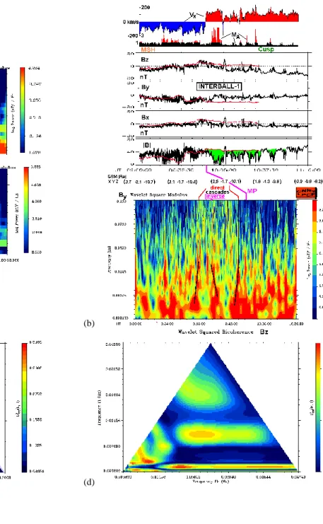
One of the challenging problems is to distinguish dynamic interactions of the solar wind with MP from the local TBL turbulence. To shed light on this problem, we display in Fig. 1a wavelet spectrograms for magnetic GSE components Byfrom Geotail in SW and from the Interball-1 passage from SW to the magnetosphere (bowshock (BS), MSH and MP crossings are marked on the bottom of Fig. 1a). Wavelet anal-ysis serves to investigate turbulent signals and short-lived structures. In order to examine transient nonlinear signals in the TBL, we have performed the wavelet transform with the Morlet wavelet:

W (a, t )

=CX nf (ti)exp(i2π(ti−t )/a − (ti −t )2/2a2) o

, (1) where C has been chosen so that the wavelet transform am-plitude |W (a, t )| is equal to the Fourier one (see Consolini and Lui, 2000 and references therein for details). When this wavelet shows the single peak at the frequency f = 1/a, a wavelet characteristic scale may be read as representing a frequency f = 1/a ± f/8. Returning to Fig. 1a, the time lag between Geotail and Interball-1 should be in the limit of 5–20 min (see Dubinin et al., 2001). In the low-frequencies, BS (lower panel) differs clearly from the si-multaneous SW perturbations, while the first upstream wide-band burst looks very similar on both panels. In the middle

of MSH, at ∼ 08:30 UT, another disturbance practically coin-cides with that of SW, and the low-frequency part is strength-ened in MSH. At 09:00–10:50 UT in the MP vicinity wide-band Interball-1 fluctuations are seen, most of them have no counterparts in SW. Note the multiple spectral maxima in this region, which we call “TBL” (see Savin et al., 1998, 2001, 2002a, b), which are tied in a complicated manner. Simi-lar to frequencies higher than 0.7 mHz, the disturbances in the TBL have a higher level and a different frequency depen-dence, as compared with MSH; we think that the MSH is not the major source for the fluctuations in TBL.

We blow-up the TBL wavelet spectrogram (both in time and frequency) on the lower panel of Fig. 1b. The spectro-gram clearly outlines wavetrains at different frequencies si-multaneously that can be seen up to several Hz (not shown). The linkage between the maxima represents a feature of cas-cade processes. Direct/reverse (i.e. high- or low-frequency fluctuations appear first) cascade-like events can be recog-nized. Black lines highlight representative examples. The re-verse cascade from 0.025 to 0.00625 Hz at ∼ 10:52 UT might converge with the direct one from 0.004 Hz. Several high frequency branches are seen frequently. We mark the ap-proximate MP position in the middle of Fig. 1b. In the pres-ence of the intensive fluctuations it is not easy to define it. So, we present magnetic field data and the GDCFM predic-tions (red lines) on the middle panels of Fig. 1b, using Geo-tail magnetic field in SW as input (see Dubinin et al., 2001 and references therein). We identify the time, which sep-arates average the MSH and magnetospheric fields, as the MP (the MSH region is where the data are close to the GD-CFM, red curves). Note also the large-scale magnetic field depletion at 09:57–10:05 UT, which is just inside MP (cf. Vx sign). The heated MSH plasma and plasma sheet ions are mixed in this “plasma ball” (Savin et al., 2002b). To es-timate the scale of this diamagnetic “plasma ball” we have found the de Hoffman-Teller frame (dHT; see e.g. Savin et al., 2002b) at 09:56:54–10:00:02 UT with GSE veloc-ity VH T = (139, −45, 18) km/s, regression coefficient of (V × B) versus (VH T ×B) R = 0.999, and small accel-eration aH T = (−0.06, −0.06, 0.14) km/s2. Existence of such a good dHT frame implies that the “ball” passes In-terball with ∼ VH T and thus its scale can be estimated at ∼5 Re. While the plasma in the “ball” moves sunward, it cannot take into account the unique large-scale reconnection since the stress balance checking fails on this interval (cf. Savin et al., 2002b).

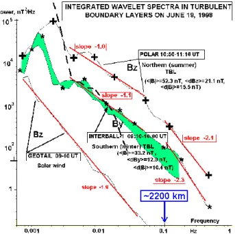
For the quantitative comparison of the TBL properties with the SW ones, we present characteristic spectra in Fig. 2 from the core TBL intervals at 09:10–10:00 and 09:53–11:00 UT (shadowed in between), and compare them with the Geo-tail SW data at 09:00–10:00 UT and with that for the north-ern TBL entered by Polar at 10:50–11:10 UT (Savin et al., 2002b). The maximum at ∼0.0014 Hz corresponds to the time lag between MA spikes on the second top panel of Fig. 1b, which is close to the Alfv´en transition time for traversing the magnetopause between the cusp regions or from the MP to the ionosphere. Two characteristic negative

(a)

(b)

(c) (d)

(e)

Fig. 1. (a) Wavelet spectrogram (By,) for Geotail in SW and for Interball-1 inbound TBL/MP on 19 June 1998. Bowshock (BS), MSH and MP are marked at the bottom. (b) Wavelet spectrogram (By, bottom) and GSM magnetic field for Interball-1 inbound TBL/MP on 19 June 1998. Red lines – GDCFM model (see text for details); upper panels: ion speed Vxand Alfv´en Mach number MA. (c) Bi-spectrogram of

Bxin TBL at 09:16–09:50 UT on 19 June 1998 (see text). (d) Bi-spectrogram of Bzfor the virtual spacecraft crossing of the model current sheet (see Figs. 1e and 4 and text for details). (e) Helicity for the model current sheet crossing by virtual spacecraft (the trace is shown by the gray arrow, see text and Fig. 4); at the right – linear color-coded scale.

446 S. Savin et al.: On the properties of turbulent boundary layer over polar cusps

Fig. 2. Wavelet integrated spectra in the northern/southern TBL and

in the SW.

slopes are actually seen: ∼ 2.3 at 0.1–0.5 Hz and ∼ 1.1 at 0.004–0.05 Hz (note similar slopes at the upper trace with the crosses from Polar). The different slope of −1.9, seen by Geotail in SW, and the absence of any maximum in the Geotail data, demonstrate that the dominant processes in the TBL in this event are the local and inherent ones (cf. Fig. 1a), despite that the average field is following the SW, as demon-strated by the model to data comparisons in Fig. 1b. Interball-1 magnetic spectra for 0.004–0.5 Hz in the outer cusp at 09:53–11:00 UT (the shadowed curve without asterisks) have a similar shape to that of the core TBL (trace with asterisks), while the slope at 0.004–0.05 Hz of 1.3 is slightly higher. At 09:55–10:30 UT, the slope from Interball-1 at 0.1–0.5 Hz is the same as in the TBL just outside the MP. The charac-teristic power at low frequencies in the core region is about twice that just inside MP (at 09:10–10:00 UT, the difference is shadowed). Shifting the interval to 09:56–10:08 UT re-duces the peak at ∼ 0.0014 Hz by factors of 2 to 3, but does not change the rest of the spectrum much. This is in strong contrast to that seen in the summer TBL, where the power drops by the order of magnitude in the outer cusp (see Savin et al., 1998b, 2002a, b). The difference in the power for Polar and Interball spectra in Fig. 2 of about one order of magni-tude cannot be attributed to the higher average magnetic field on Polar (∼ in 1.6 times). We suggest that the power excess may be due to patchy reconnection of the nearly anti-parallel fields on Polar (cf. Dubinin et al., 2001). The reconnection of the average, nearly perpendicular fields in the Interball case is hardly operative, but fluctuating fields can still reconnect as the ion speed Vxand MAspikes infer (see 2 top panels in Fig. 1b). In the latter case, the average field is not annihi-lated and the energy input into turbulence is thus lower.

An-other characteristic TBL feature is the fact that the standard variances hdBzi and hdByi are higher than that of the field magnitude hd|B|i (see text in Fig. 2). It implies that the trans-verse magnetic fluctuations dominate over the compressible ones (cf. Savin et al., 1998b, 2001, 2002a, b). To estimate the scale of the kink in Fig. 2, we have found the dHT frame with GSE velocity VH T = (−156, 82, −121) km/s and re-gression R = 0.993 at 09:35:31–09:39:03 UT, which yields for the kink L ∼ 2200 km, as marked in Fig. 2.

To investigate if the wave trains in TBL are really cou-pled by the cascade-like nonlinear processes, we have studied the magnetic spectral bicoherence using a wavelet approach, which is able to resolve phase coupling in short-lived events and pulses (see e.g. Consolini and Lui, 2000 and references therein). We use SWAN software from LPCE/CNRS in Or-leans for the wavelet analysis that defines the bicoherence as: b2(a1, a2) = |B(a1, a2)|2/ nX |W (a1, ti)W (a2, ti)|2 X W (a, ti)|2 o ,(2)

with B(a1, a2) being the normalized squared wavelet

bi-spectrum: B(a1, a2) =

X

W ∗ (a, ti)W (a1, ti)W (a2, ti). (3) The W (a, t ) is wavelet transform according to Eq. (1) and the sum is performed by satisfying the following rule:

1/a = 1/a1+1/a2, (4)

which correspond to a frequency sum rule for the 3-wave process, f = f1+f2.

The bicoherence has substantial value only if three pro-cesses, with the highest frequency being the sum of the lower frequencies, are phase coupled (cf. Consolini and Lui, 2000). The simplest such case is the harmonic generation due to quadratic nonlinearity, namely the second and third harmonic generation with 2f = f + f , and with 3f = 2f + f . As the harmonics are present in any nonlinear wave pulse and do not represent phase coupling of the different waves, we will ignore them in the future analysis. We assume that the most powerful nonlinear 3-wave process (excluding the har-monics) in the TBL decays, which requires the third order nonlinearity in the system. The weaker, higher order nonlin-ear effects, which also might contribute in the TBL physics, are beyond the scope of this paper and will be addressed in future studies.

In Fig. 1c, we present an Interball bicoherence spectro-gram for the GSE Bx component from the TBL interval at 09:16–09:50 UT. All features, visible in Fig. 1c, are present both in the bi-spectra of other components from Interball, and in the respective bi-spectrograms from Polar (Savin et al., 2002b). The frequency plane (fL, fK) is limited by the signal symmetry considerations and by the frequency interval of the most characteristic TBL slope of about −1 in Fig. 2. The bicoherence spectra in Fig. 1c display, most probably, 3-wave processes with the cascade-like features, that are cen-tered at ∼ 0.005 and ∼ 0.0 Hz. We assume cascade signa-tures in Fig. 1c when at the sum frequency, f = f1+f2,

Fig. 3. Interball-1 encounter of a double current sheet in the TBL

on 19 June 1998. From bottom: Magnetic field magnitude |B| (variation matrix eigenvalues are printed at the right side); Normal component and its unit vector in GSE; The same for intermediate component; The same for maximum variance component; Magnetic vector hodograms in maximum/intermediate (left) and maximum/ minimum (right) variance frames.

the bicoherence has a comparable value with that at the point (f1, f2). In the case of the horizontal-spread maximum, it

implies that the wave at sum frequency interacts with the same initial wave at frequency f1 in the following 3-wave

process: f3=f1+f, etc. Returning to Fig. 1c, we suggest

that, in general, the energy flows from the lower to higher fre-quency regions with the slope ∼ 2.3, which is characteristic for the developed MHD turbulence (cf. Zelenyi and Milo-vanov, 1999). Assuming that the cascade origin corresponds to the highest bicoherence amplitude, one can infer a cas-cade (0.005 + 0.13) towards the low and high frequencies in Fig. 1c. In Fig. 2, the frequency 0.12–0.14 Hz corresponds to the spectrum kink. In Fig. 1c, one more cascade-like hori-zontal maximum starts from (0.02 + 0.13) Hz towards higher frequencies, noting also a weaker one at (0.07 + 0.13) Hz. In TBL we have found a variety of magnetic field rotations, ac-companied by vortex-like loops and demagnetized “diamag-netic bubbles” (DB; cf. Savin et al., 1998a, b, 2001, 2002a,

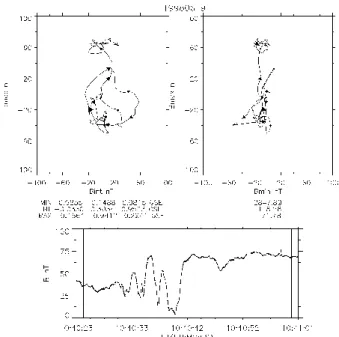
Fig. 4. Polar encounter of a current sheet in TBL on 19 June 1998. From bottom: Magnetic field magnitude; Mag-netic vector hodograms in maximum/intermediate (left) and max-imum/minimum (right) variance frames.

b). In Fig. 3, we display a characteristic example of the mag-netic field rotation back and forth in the inner TBL at 10:18– 10:19 UT on 19 June 1998 on Interball-1. The magnetic field is presented in the local minimum variance frame (with Bn on second bottom panel being the minimum variance com-ponent, Bmon third top panel – medium one, Bl on second top panel – maximum one), the eigenvalues (presented on the bottom panel in nT2) reasonably well define this local frame. Bnon average, is close to zero, representing a feature of tangential discontinuities, while quasi-regular fluctuations are superimposed. At the inbound transition at 10:18:40 UT, a DB is visible, confirming with the Harris-like equilibrium in the current layer with sharp field rotation (B¨uchner et al., 1998). However, the outbound rotation does not contain a DB. The magnetic field vector hodogram on the top panel in Fig. 3 exhibits loops at different scales superimposed on the main field rotation. It also indicates cascade-like pro-cesses (cf. Figs. 1a–c). The time lag between current sheets corresponds to the inverse frequency of the horizontal max-imum at fL ∼0.02 Hz in Fig. 1c; it falls into the region of slope ∼ − 1 in Fig. 2. The maxima at fK ∼ 0.13 Hz and the spectrum kink in Fig. 2 have periods of the order of the field rotations’ periods (and of the DB). Thus, we associate the TBL spectral features with the characteristic time scales of the structures, which are similar to the ones, depicted in Fig. 3.

In about one-third of the cases in TBL, the field rota-tions contain solitons-like structures, which contain DBs. In Fig. 4, we depict a characteristic example from simultane-ous Polar data at 10:41 UT in the northern TBL (see details

448 S. Savin et al.: On the properties of turbulent boundary layer over polar cusps

Fig. 5. Statistical properties of the TBL magnetic fluctuations. (a) The tip of the magnetic vector motion in the maximum variance plane

for the TBL period (see bottom panel of Fig. 1b), λ1and λ2refer to the maximum and medium variance directions. (b) The normalized

probability distribution function of the rotation angle of the magnetic field vector in the maximum variance plane. The solid line refers to a nonlinear best fit using a symmetric Levy-stable distribution function characterized by a characteristic index α ∼ 1.17 (see also text).

in Savin et al., 2002b). The displayed transition contains a quasi-regular structure in |B| (bottom panel) enveloped by the field, the hodogram of which (top panel) resembles a 3-D spiral with increasing radius (decreasing with the distance from the main rotation). Note that the duration of the DB wave train again corresponds to the maxima at fK ∼0.13 Hz and to the spectrum kink in Fig. 2; the wave train filling the frequency of ∼ 0.35 Hz belongs to the high-slope part of the upper spectrum (with the ion cyclotron frequency be-ing ∼0.45 Hz for the average total field ∼ 30 nT through the structure, see Fig. 4). One needs high-time resolution plasma moments to compare properly such transitions with interme-diate/slow shocks from kinetic simulations by, for example, Karimabadi et al. (1995), while we should mention that the |B| drop by the order of magnitude does not appear in the simulations.

In Fig. 5, we present the results of a statistical study of the TBL fluctuation behavior. The tip of the magnetic vector motion in Fig. 5a is shown in the maximum variance plane for the TBL period. The field direction variance looks rather random. Visible dividing on the upper and lower parts is due to both changes in the average direction of the SW-induced field (red traces from GDCFM in Fig. 1b) outside MP and due to the different magnetospheric-controlled field direction inside the MP. Note also the difference in the TBL spectral shapes inside and outside the MP (shadowed traces in Fig. 2). Figure 5b shows the normalized distribution function of the rotation angle of the vector in the maximum variance plane. There is the evidence of non-Gaussian statistics at the high rotation angles, which is seen as a nonlinear best fit using a symmetric Levy-stable distribution function characterized by a characteristic index α ∼ 1.17 (the solid line). The Gaus-sian distribution should look like a parabola (a Levy-stable distribution function with a characteristic index α = 2) in Fig. 5. Most probably, the departure from a Gaussian dis-tribution should be attributed to the existence of the

struc-tures with small-scale current sheets, such as in Figs. 3 and 4. Thus, these soliton-like structures, while appearing as ca-sual crossings of MP, as surface waves or as reconnection pulses (Dubinin et al., 2001; Savin et al., 2002b), control the spectral shape of the TBL turbulence and change its statisti-cal properties.

3 Discussion and conclusions

We have demonstrated that the TBL has persistent features at the high latitude MP (cf. Sandahl et al., 2000). The presence of disturbances, weakly dependent on the IMF, indicates the significance of the MSH flow is direct interaction with the high latitude obstacle – the outer cusp throat (Savin et al., 2001, 2002a, b).

The super-Alfv´enic flows in front of the MP (red-shadowed in 2 top panels of Fig. 1b) indicate that the steady merging is hardly possible (La Belle-Hamer et al., 1995). In-stead, Dubinin et al. (2001) and Savin et al. (2002b) assume that the quasi-regular jets at 10:00–11:00 UT in Fig. 1b repre-sent cusp counterparts of patchy merging. These spiky cusp jets constitute a part of the flow is coherent interactions, dis-cussed above (Figs. 1a–c). In particular, the flow’s repetition quasi-periodicity in Fig. 1b corresponds to the spectral max-ima at few MHz in Fig. 1c. The difference between VH T and the average ion bulk velocity in the jet vicinity is in the limit of the bulk velocity variations (deviation < 16◦), which should be a characteristic feature for standing structures in the cusp plasma frame. So, we could infer the space rather than time resonance pattern at the MSH/cusp interface. If VH T is at 107◦to the surrounding magnetic field, then one can obtain an estimate of the transverse scale of the jet of ∼2 Re.

To check if the visible features in the TBL can be ac-counted for by crossings of reconnected current sheets, we compare the experimental data with that of the virtual

satel-Fig. 6. Virtual satellite trace through the model reconnected current sheet (right panel, see also Figs. 1d and 1e, and text) and hodogram of

magnetic field, visible on the virtual satellite in the model (Y Z) plane.

lite in a model current sheet. We use results of kinetic sim-ulations by B¨uchner et al. (1998) of the reconnection, de-veloped in the current sheet between anti-parallel magnetic fields. We depict a representative field picture on the right panel in Fig. 6. In the initial state, the current sheet with gradients in the Z direction and the external field in the X di-rection has neither Y -dependence, nor a By-component; no average change in the plasma density across the current sheet has been inferred. In Fig. 6 we present the 2-D-case with no Y-dependence and the periodic picture in the X direction (i.e. one period in X is displayed). After ∼ 15 ion gyro-periods in the external field, the current sheet divides into reconnected X- and O-lines: in Fig. 6, one X-line and two halves of the O-lines are shown. Unlike MHD, in kinetic simulations a strong By-component is generated, which leads to the ap-pearance of helicity maxima along the X-axis, as is shown in Fig. 1e for the same region as in Fig. 6 (right panel); the X and Z axes are normalized here by the half-width of unper-turbed current sheet. In Fig. 1e, across the sheet (along Z, at Z ∼0) and at some distance along it (along X at Z ∼ (+/−) half-width of the current sheet), the neighbor helicity max-ima have opposite signs; namely, this leads to the registra-tion of loops in the magnetic field hodograms on the virtual satellite, as one can see on the left panel in Fig. 6. One full loop in the hodogram is seen only if the virtual satellite orbit crosses two vortices with opposite helicities, as shown by the orbit traces in Fig. 1e and Fig. 6. A trace along the diagonal of Fig. 1e (crossing two maximum with the same polarities) would result in “S-shaped” hodograms (see e.g. Dubinin et al., 2001). Sliding along the X-axis close to the plane with Z ∼0 provides the appearance of multiple loops in the data, similar to Fig. 4. On the other hand, the latter case from Po-lar could be also accounted for by a 3-D vortex, simiPo-lar to the simulated vortices in B¨uchner et al. (1998). Note also that the crossing of a single 2-D vortex would be seen on a satellite as part (maximum half) of a loop in the hodogram.

In Fig. 2, we display the wavelet spectrum from the model By-component by a dashed line (the virtual satellite data

from the trace shown in Fig. 6 and Fig. 1e) onto the mea-sured spectra. While the virtual satellite speed (and thus fre-quency) contains an arbitrary factor, some similar features can be stated: (i) a sharp increase in power at low frequen-cies, which corresponds both to the transverse scale of the virtual current sheet at the nonlinear state (i.e. ∼ vertical size of the right panel in Fig. 6) and to the distance between O(X)-lines in the X direction, i.e. to the distance between the helicity maxima in the X direction in Fig. 1e; (ii) a kinked spectrum at higher frequencies, where the kink frequency is close to the inverse time-of-flight of the single maximum in helicity in Fig. 1e. A possible reason for the discrepancy between the experimental and model spectra at higher fre-quencies is the limitation in the model grid size.

Finally, we compare the experimental Bx (Fig. 1c) and model Bz(Fig. 1d) bi-spectrograms, with the GSE X direc-tion at the MP being the closest to the current sheet normal, as the model Z axis is. The presence of two sets of hor-izontal maxima in fL constitutes the general similarity in the bi-spectrograms. In the model the lower maximum in-fers synchronization of the nonlinear (presumably 3-wave) processes inside the reconnected current sheet at the nonlin-ear state; similar cascade-like synchronization at the higher frequency (upper horizontal maximum) relays with the in-dividual vortex-like structure (single helicity maximum in Fig. 1e). The third (higher) maximum in fL is also visible in both Figs. 1c and d. Similar to the model is lower fre-quency maximum in fLin Fig. 1d, the experimental one in Fig. 1c coincides with the low-frequency edge of the spectral slope of ∼ − 1. We attribute this maximum to the large-scale wave structures, which synchronize TBL processes globally. As MSH flows interact with the MP, which has gradients in its normal direction that are much sharper than in the parallel ones, those larger-scale waves should resemble the surface ones (Savin et al., 2001, 2002a, b). Thus, the model data are rather similar to the ones discussed above (Fig. 1c): (i) while the magnetic field transitions in Fig. 3 might seem to be independent, they seek to synchronize a number of 3-wave

450 S. Savin et al.: On the properties of turbulent boundary layer over polar cusps

processes inside (the similarity in the lower frequency max-ima in Figs. 1c and d); (ii) the quasi-coherent structures (cf. Figs. 4, 6 and Fig. 1e) have the decay-like nonlinear phase coupling, both with global structures (e.g. reconnection sites or “magnetic islands”, i.e. the model O-lines) and with the higher frequencies.

In spite of the complicated time-dependent geometry (as compared with the plain quasi-stationary one in the model), the sharp density gradients in the TBL, and the limitations in the model grid size, etc., we have shown that a substantial number of the TBL turbulence features can be understood by comparison of the experimental data with the model of ki-netic reconnected current sheet at the nonlinear state. Proba-bly, the evolution of nonlinear structures in the hot inhomo-geneous plasma weakly depends on the initial disturbances after exceeding some amplitude or scale thresholds. For ex-ample, Chmyrev et al. (1988) have shown that after thinning to the ion gyroradius scale, current sheets tend to split into the vortex streets, since this state has lower energy as com-pared with the homogeneous planar current sheet. The char-acteristic scales of the TBL turbulence are shown to reach the scales of a few km, i.e. several electron inertial lengths c/ωpe (Savin et al., 1998b). This infers violation of the frozen-in field condition and could also be treated as a feature of the local reconnection near the cusp. The operation of the bursty reconnection for the locally anti-parallel fields over the cusp is in agreement with a number of studies, and the experimen-tal evidences for the permanent by-product reconnection of the TBL is strongly fluctuating fields are seen as well (see e.g. Savin et al., 1998b, 2001, 2002a, b; Merka et al., 2000; Onsager et al., 2001; Dubinin et al., 2001).

Thus, we regard the quasi-coherent structures as residuals of the nonlinear evolution of current sheets; the “diamagnetic bubble” presence supports this suggestion, since the field de-pletions in the middle of equilibrium current sheets is widely accepted and a number of modelings predict the small-scale depletions at nonlinear current states (see e.g. B¨uchner et al., 1998; La Belle-Hamer et al., 1995). As a result of the multi-scale reconnection, field lines are connected through the TBL in a statistical sense, without the opportunity to trace individual field lines in the inhomogeneous non-equilibrium 2-phase medium, with one phase being the frozen-in “MHD” plasma and the other one represented by unmagnetized DB embedded in the nonlinear current sheets and magnetic vor-tices. The latter “phase” (in the statistical sense) provides the power-law spectra with the slope of ∼ − 1, which implies a special type of translation symmetry of the fluctuations. The quasi-coherent solitons (e.g. similar to that of Figs. 3 and 4) are breaking the Gaussian statistics, most probably due to the TBL intermittency; the above mentioned spectral slope of ∼ − 1 is consistent with this suggestion. We will devote a separate paper to the further study of the intermittency in the TBL.

The spectral shapes and dynamic wavelet spectra demon-strate the inherent character of the TBL fluctuations, where the most characteristic ones have no counterpart in SW. We propose that MSH is also not the dominant source of the

TBL turbulence, while the most powerful perturbations in SW and MSH certainly modulate/trigger the dynamic pro-cesses in the TBL. The cascade-like wavelet and bicoher-ence spectrograms infer coherent interaction between wave trains, while the disturbances seem to be random in wave-forms. Quasi-coherent large-scale structures, which organize phase coupling throughout the entire TBL, can result from the inverse cascades of the local wave trains (see Fig. 1c and related discussions). The local wave trains originate from the interaction of the disturbed MSH flows with the MP, where the interaction includes local reconnection as a part of it. The TBL disturbances modulate the incident MSH flow in a self-consistent manner, being globally organized by the phase coupling with the long-scale variations. So, the circle is closed: the TBL seems to be a scale multi-phase self-organized system of interacting nonlinear waves. It infers qualitative difference from the traditional approach when the MSH/cusp interaction is regarded as the additive sum of the magnetospheric reactions with the solar wind or MSH disturbances. Note also that the long-term correlation is suggestive for systems out of equilibrium near the critical point (cf. Consolini and Lui, 2000). The kinked TBL spec-tra with characteristic slopes remarkably resemble that in the near-Earth neutral sheet in the state of the self-organized crit-icality (see e.g. Zelenyi and Milovanov, 1999).

In conclusion, the soliton-like current sheets, often ac-companied by quasi-coherent substructures and “diamag-netic bubbles”, control the spectral shape of the TBL turbu-lence in the range of ∼ (0.005–0.1) Hz and change its sta-tistical properties. These properties of the turbulent bound-ary layer should define the energy and mass transport in the significant region of the magnetosphere (Savin et al., 2001), through which the solar wind plasma is penetrating inside the magnetopause.

Acknowledgements. We appreciate D. Lagoutte and his colleagues

from LPCE/CNRS in Orleans for providing the SWAN software. We thank the Geotail MFI team for high-resolution Geotail mag-netic field data and also V. Romanov, I. Dobrovolsky and A. B. Belikova for help in the data processing. Work was partially sup-ported by International Space Science Institution, and by grants INTAS/ESA 99-1006, INTAS-2000-465, EST.CLG 975277, KBN 8T12E04721 and by Humbolt Foundation.

References

B¨uchner J., Kuska, J. P., Nikutowski, B., Wiechen, H., Rustenbach, J., et al.: Three-dimensional reconnection in the Earth’s mag-netotail: simulations and observations, Geophysical Monograph, 104, AGU, (Eds) Horwitz, J. L., Gallagher, D. L., and Peterson, W. K., Washington D. C., 313–325, 1998.

Chen, S.-H., Boardsen, S. A., Fung, S. F., Green, J. L., Kessel, R. L., Tan, L. C., Eastman, T. E., and Craven, J. D.: Exterior and inter ior polar cusps: Observations from Hawkeye, J. Geophys. Res., 102 (A6), 11 335, 1997.

Chmyrev, V. M., Bilichenko, S. V., Pokhotelov, O. A., Marchenko, V. A., Lazarev, V. I.: Alfv´en vortices and related phenomena

in the ionosphere and magnetosphere, Physica Scripta, 38, 841– 854, 1988.

Consolini, G. and Lui, A. T.: Symmetry breaking and nonlinear wave-wave interaction in current disruption: possible evidence for a phase transition, in Magnetospheric Current Systems, Geo-physical Monograph, 118, AGU, Washington D. C., 395-01, 2000.

Dubinin, E., Skalsky, A., Song, P., Savin, S., Kozyra, J., et al.: Polar-Interball coordinated observations of plasma characteris-tics in the region of the northen and southern distant cusps, J. Geophys. Res., 106, accepted, 2001.

Fedorov, A., Dubinin, E., Song, P., Budnick, E., Larson, P., and Sauvaud, J. A.: Characteristics of the exterior cusp for steady southward IMF: Interball observations, J. Geophys. Res., 105, 15 945–15 957, 2000.

Haerendel, G. and Paschmann, G.: Entry of solar wind plasma into the magnetosphere, in: Physics of the Hot Plasma in the Mag-netosphere, (Eds) Hultqvist, B. and Stenflo, L., 23, Plenum, NY, 1975.

Haerendel, G.: Microscopic plasma processes related to reconnec-tion, J. Atmos. Terr. Phys., 40, 343–353, 1978.

Karimabadi, H., Krauss-Varban, D., and Omidi, N.: Kinetic struc-ture of intermediate shocks: implications for the magnetopause, J. Geophys. Res., 100-11, 957, 1995.

Klimov, S. I., Nozdrachev, M. N., Triska, P., et al.: Investi-gation of plasma waves by combined wave diagnostic device BUDWAR PROGNOZ-10-INTERCOSMOS, Cosmic Research (transl. from Russian), 24, 177, 1986.

Lundin, R., Woch, J., and Yamauchi, M.: The present understanding of the cusp, in Proceedings of the Cusp Workshop, European Space Agency, Spec. Publ., ESA SP-330, 83–95, 1991. La Belle-Hamer, A. L., Otto, A., and Lee, L. C.: Magnetic

recon-nection in the presence of sheared flow and density asymmetry: application to the Earth’s magnetopause, J. Geophys. Res., 100, 11 875–11 889, 1995.

Maynard, N. C., Savin, S., Erickson, G. A., Kawano, H., et al.: Observations of fluxes of magnetosheath origin by Polar and In-terball at high latitudes behind the terminator – relationships to the magnetospheric “sash”. J. Geophys. Res, 104, 6097, 2001. Merka, J., Safrankova, J., Nemecek, Z., Fedorov, A., Borodkova,

N., Savin, S., and Skalsky, A.: High altitude cusp: Interball ob-servations, Adv. Space Res., 25, 7/8, 1425–1434, 2000. Onsager, T. G., Scudder, J., Lockwood, M., and Russell, C. T.:

Re-connection at the high latitude magnetopause during northward IMF conditions, J. Geophys. Res., 106, in press, 2001.

Paschmann, G., Haerendel, G., Sckopke, N., et al.: Plasma and magnetic field characteristics of the distant polar cusp near lo-cal noon: The entry layer, J. Geophys. Res., 81, 2883, 1976. Petrinec, S. M. and Russell, C. T.: An examination of the effect

of dipole tilt angle and cusp regions on the shape of the dayside magnetopause, J. Geophys. Res., 100, 9559–9566, 1995. Sandahl, I., Popielavska, B., Budnick, E. Yu., Fedorov, A., Savin,

S., Safrankova, J., and Nemecek, Z.: The cusp as seen from Inter-ball, Proceedings of Cluster II Workshop. Multiscale/Multipoint Plasma Measurements, Imperial College, London, 22–24 Sept. 1999, ESA/ SP-499, 39–45, 2000.

Savin, S., Romanov, S., Fedorov, A., Zelenyi, L., Klimov, S., et al.: The cusp/magnetosheath interface on 29 May 1996: Integball-1 and Polar observations, Geophys. Res. Lett., 25, 2963–2966, 1998a.

Savin, S., Borodkova, N., Budnik, E., Fedorov, A., Klimov, S., et al.: Interball tail probe measurements in outer cusp and bound-ary layers, in Geospace Mass and Energy Flow: Results from the International Solar-Terrestrial Physics Program, (Eds) Hor-witz, J. L., Gallagher, D. L., and Peterson, W. K., Geophysical Monograph 104, AGU, Washington D. C., 25–44, 1998b. Savin, S. P., Zelenyi, L. M., Romanov, S. A., Klimov, S. I., Skalsky,

A. A., et al.: Tubulent Boundary layer at the Border of Geomag-netic Trap, JETP Letters, 74, 11, 547–551, 2001.

Savin, S., Zelenyi, L., Rauch, J. L., Romanov, S., Sandahl, I., et al.: Magnetosheath/cusp interface, Ann. Geophysicae, in press, 2002a.

Savin S., Zelenyi, L. M., Maynard, N. C., Sandahl, I., Kawano, H., et al.: Multi-spacecraft Tracing of Turbulent Boundary Layer, Adv. Space Res., 24, (COSPAR-2000 Proceedings) in press, 2002b.

Smith, M. F. and Lockwood, M.: Earth’s magnetospheric cusps, Rev. of Geophys., 34, 233, 1996.

Spreiter, J. R. and Briggs, B. R.: Theoretical determination of the form of the boundary of the solar corpuscular stream produced by interaction with the magnetic dipole field of the Earth, J. Geo-phys. Res., 67, 37–51, 1962.

Zelenyi, L. M. and Milovanov, A. V.: Multiscale magnetic struc-ture of the distant tail: self-consistent fractal approach, in: New Perspectives on the Earth Magnetotail, Geophysical Monograph, 105, AGU, Washington D. C., 321–338, 1999.