Investigation of Dipole Sources in the Biceps Brachii as Upper Limb Position is Modified

(1)

UNIVERSITÉ DE MONTRÉAL

INVESTIGATION OF DIPOLE SOURCES IN THE BICEPS BRACHII AS

UPPER LIMB POSITION IS MODIFIED

PEYMAN AGHAJAMALIAVAL DÉPARTEMENT DE GÉNIE ÉLECRIQUE ÉCOLE POLYTECHNIQUE DE MONTRÉAL

MÉMOIRE PRÉSENTÉ EN VUE DE L’OBTENTION DU DIPLÔME DE MAÎTRISE

(GÉNIE ÉLECTRIQUE) AOÛT 2015

(2)

UNIVERSITÉ DE MONTRÉAL

ÉCOLE POLYTECHNIQUE DE MONTRÉAL

Cette thése intitulée:

INVESTIGATION OF DIPOLE SOURCES IN THE BICEPS BRACHII AS

UPPER LIMB POSITION IS MODIFIED

présenté par : AGHAJAMALIAVAL Peyman

en vue de l’obtention du diplôme de : Maîtrise ès sciences appliquées

a été dûment accepté par le jury d’examen constitué de : M. BRAULT Jean-Jules, Ph. D., président

M. CORINTHIOS Michael, Ph. D., membre et directeur de recherche M. MATHIEU A. Pierre, Ph. D., membre et codirecteur de recherche M. SAUVÉ Rémy, Ph. D., membre

(3)

DEDICATION

Dedicated to my lovely parents Nahid and Latif, my beloved soul mate Eli, and my fantastic grandmas Soofi and Fezeh.

(4)

ACKNOWLEDGEMENTS

I would like to express my deepest gratitude and appreciation to my director of research Professor Michael J. Corinthios and my co-director Professor Pierre A. Mathieu for their continuous supports, contribution, guidance, and constant encouragement throughout this research work. It has been an honour and pleasure to work with them. Their immense patience and incredible meticulous consideration have left indelible effect on me. The financial support through this research is also greatly acknowledged.

I would also like to express my deepest gratefulness to Professor Michel Bertrand for his supports, guidance, contribute, and encouragement.

I am most grateful to the members of my committee, Professor Jean-Jules Brault and Professor Rémy Sauvé for their time, encouragement, and expertise throughout this project.

My special thanks to the faculty and staff of Electrical Department at Polytechnique de Montréal and Institute of Biomedical Engineering of Université de Montréal who have been always helpful and co-operative.

I would like to thank Etienne Bouffard-Cloutier and Pierre-Yves Sirois C., students from Polytechnique who worked at EMG lab with me during their summer internship. I also gratefully acknowledge Jean L. Laurier for his contribution in our weekly meetings throughout this project.

Last but not least, I would like to thank my parents, Nahid Vafai and Latif Aghajamaliaval, and my beloved wife Elmira for their endless support, encouragement and prayers. Without their support this work would not have been possible.

(5)

RÉSUMÉ

Pour une personne ayant subi une amputation au niveau du bras, les prothèses myoélectriques modernes offrent la possibilité de reproduire plusieurs mouvements nécessaires dans la vie quotidienne. Pour ce faire, plusieurs signaux de contrôle sont toutefois nécessaires pour pouvoir en bénéficier pleinement. Dans la partie supérieure du bras, le biceps brachial (BB) est un muscle important où on trouve sur sa surface intérieure des divisions suggérant la présence de 3 compartiment dans le chef court (SH) et 3 dans le chef long (LH). Comme chacun d'eux est innervée par une branche nerveuse, il est possible que ces compartiments puissent être activés individuellement permettant ainsi d’obtenir jusqu'à six signaux de contrôle pour se servir d’une prothèse myoélectrique. Pour explorer cette possibilité, quelqu’un de notre groupe (NN) avait il y a 3 ans, fait des enregistrements de 10 signaux électromyographiques (EMG) obtenus au-dessus du biceps droit de jeunes sujets. Ces derniers, en position assise ou debout avec la main en différentes positions, avaient mis leur biceps en contraction isométrique et isotonique. Pour chaque position testée, la valeur quadratique moyenne (RMS) de chacun des 10 signaux obtenus lors d’une contraction a été calculée à leur moyenne obtenue à partir de 3 essais consécutifs. Avec une méthode de détection de crêtes parmi chaque ensemble de 10 valeurs RMS, ont a associé la présence de dipôles à l'intérieur du biceps. Pour vérifier comment les caractéristiques des dipôles identifiés permettaient de reproduire les résultats expérimentaux, des simulations ont été réalisées avec le logiciel COMSOL. Le bras a été modélisé par un cylindre à 4 couches concentriques représentant la peau, la couche de graisse, le tissu musculaire et l’os et la conductivité de ces tissus à 100 Hz a été utilisée dans les calculs de simulation et l’anisotropie du tissu musculaire a été prise en considération. Faisant l’hypothèse que les 6 compartiments à l’intérieur du biceps sont de surface égale et séparés par des parois verticales, la plupart des dipôles identifiés se sont retrouvés dans un de ces compartiments ou à la démarcation entre deux d’entre eux. Quelques dipôles se sont toutefois retrouvés à l’extérieur des contours du biceps. En position assise, les dipôles se sont retrouvés plus fréquemment dans les compartiments du chef court (SH) alors qu’en positon debout, ils étaient plus nombreux à se retrouver dans ceux du chef long (LH). Les changements dans la position de la main ne semblent pas induire un déplacement important de la position des dipôles. Dans les positions testées, il ne semble pas possible d'activer un seul compartiment du biceps à la fois. On espère que des résultats plus satisfaisants pourront être obtenus avec des données obtenues dans d’autres positions expérimentales qui n’ont pas encore été analysées. Sinon, il sera nécessaire

(6)

de recourir à un traitement de signal afin d'obtenir du biceps plus que les deux signaux de contrôle: un pour chacun des deux chefs de ce muscle.

(7)

ABSTRACT

For an upper arm amputee person, modern myoelectric prostheses offer the possibility to produce many movements needed in a daily life. To do this, various control signals are needed to be able to fully take benefit from them. In the upper arm, the biceps brachii (BB) is an important muscle where in its inner surface, divisions suggest the presence of 3 compartment in its short head (SH) and 3 in its long head (LH). Since each of them is individually innervated by a nerve branch, there is a possibility that they could be activated independently to produce up to 6 control signals for operating a myoelectric prosthesis. To explore that possibility, three years ago, someone of our group (NN) collected 10 electromyographic (EMG) signals across the right biceps of 10 healthy young subjects. While either seated or standing up with the arm in different positions, they produced isometric and isotonic contractions of their biceps. For each tested position, the mean square (RMS) of each of the 10 signals obtained during a contraction was calculated a mean set was obtained from three consecutive contractions. With a peak detection method, the presence of dipoles within the biceps was associated to each mean set of 10 RMS values. To check how well the identified dipoles could reproduce the experimental data, simulations were done with COMSOL. In the software, the upper arm was modelled as a cylinder composed of 4 concentric layers representing the skin, the fat layer, muscular tissue and the bone and conductivity values of these tissues at 100 Hz was used in the simulations; anisotropy of muscle tissue was also considered. Assuming that the 6 compartments inside the biceps were of equal surface and separated by a vertical wall, most of the dipoles were found to be located within one compartment of the biceps or at the border of two adjacent ones. Some of the dipoles were found outside the biceps but in its vicinity. In the seated position, dipoles were more often located in a compartment of the short head (SH) while in the standing up position dipoles were most often in the long head (LH). Changes in hand position does not seem to significantly alter the dipole positions within each head. For the seating and standing up analyzed positions, it does not seem possible to individually activate a compartment. More satisfying results may be obtained from other data collected in other experimental positions that have not yet been analyzed. If this does not happen, some signal processing will be needed to extract more than one control signal from its SH and from its LH.

(8)

LIST OF TABLES

Table 2.1: Conductivity of different tissues of human body in 100 Hz. ... 17

Table 2.2: Five model configurations (from: Roeleveld et al. [35] Table 1) ... 25

Table 2.3: Composition of 5 models of Lowery et al. (Table.2 from [45]) ... 35

Table 3.1: Subjects characteristics. BMI: body mass index. ... 41

Table 3.2 : Resolution of the 2 pre-set mesh sizes that were used. ... 47

Table 3.3: The ten experimental RMS values of a subject (S2). ... 52

Table 4.1: The 10 differential simulated signals (µV) obtained when using extra Fine or Extremely Fine mesh. ... 55

Table 4.2: For each subject, errors % between experimental and simulated results in different hand postures. ... 66

Table 4.3: For the 10 subjects, total number of dipoles found within each head and outside of the biceps ... 68

Table 4.4: For the 4-layer anisotropic model, comparison of distribution of dipoles within compartments of the biceps in seated and standing up positions for the 3 hand postures. .... 72

(11)

LIST OF FIGURES

Figure 2.1: A: Upper limb bones B: Details on the elbow articulation. C: Hand postures ... 5

Figure 2.2: Upper arm muscles attached to the humerus and forearm bones. ... 5

Figure 2.3: Illustration of the biceps brachii ... 6

Figure 2.4: Structure of a muscle fiber ... 7

Figure 2.5: Sarcomeres in a relaxed condition and in a contracted state ... 8

Figure 2.6: Contraction of a muscle fiber (steps) ... 9

Figure 2.7: A: a motor unit components B: two motor units C: details of a neuromuscular junction D: various fatigue development rate ... 11

Figure 2.8: Different methods of recording EMG signals ... 12

Figure 2.9: Three types of nerve branch patterns for BB muscle.. ... 15

Figure 2.10: sketch of the posterior and anterior view of biceps brachii ... 16

Figure 2.11: Myoelectric prostheses. ... 18

Figure 2.12: A: Model of human trunk. B: Comparison of experimental and calculated results .. 19

Figure 2.13: Potentials produced by an eccentric current dipole in a finite length cylinder. ... 20

Figure 2.14: Left: surface electrodes over the BB. Right: Illustration of the image method ... 21

Figure 2.15: a. MUAP with a single peak b. MUAP with two distinguishable peaks. c: complex MUAP. ... 23

Figure 2.16: Three-layer model. from: Roeleveld et al.. ... 24

Figure 2.17: MUPs along the muscle fibers Roeleveld et al. ... 25

Figure 2.18: Same as Figure 2.17, but electrodes perpendicular to the muscle fiber. ... 26

Figure 2.19: Localisation of emission sources in a muscular cross section. ... 27

Figure 2.20: A: EMG signal; B: power spectrum of the signal C: Estimated source location D: Experimental data compared with obtained results ... 29

(12)

Figure 2.22: Left: CMG system’s chart. Right: A 3D domain Ω of Van den Doel et al. ... 31

Figure 2.23: MRI cross-section of an upper arm and many current tripole sources, of Van den Doel et al. ... 33

Figure 2.24: Finite-element multilayer model of the upper arm of Lowery et al.. ... 33

Figure 2.25: Cross section of the Loewry et al model with different bone tissue positions. ... 35

Figure 2.26: Waveform of an action potential above a fiber from Lowery et al... 36

Figure 2.27: Lowery et al. action potential of 4 models at increased fiber depth ... 36

Figure 2.28: Effect of adding bone tissue on surface potentials RMS values. ... 37

Figure 2.29: MRI cross section of a right arm and FEM model of Lowery et al.. ... 38

Figure 2.30: Anatomical based volume conductor model of Lowery et al. ... 39

Figure 2.31: Simulation results of Lowery et al for surface action potentials of a fiber located 14.5 mm under the skin surface. ... 40

Figure 3.1: Experimental conditions. ... 42

Figure 3.2: One-layer upper arm model with the 6 biceps compartments. ... 43

Figure 3.3: A: Dipoles moving within an homogeneous cylinder ... 44

Figure 3.4: Identification of the dipoles’ characteristics. ... 45

Figure 3.5: A: 1-layer model consisting only muscle in a cylinder; B: 4-layer model representing the skin, the fat layer, the muscle tissue and the humerus bone. ... 46

Figure 3.6: COMSOL multiphysics main desktop sections. ... 48

Figure 3.7: Desktop view for the parameters used to design our upper arm model... 49

Figure 3.8: A: Desktop view of different sections concerning our model. B: Geometry information for the 4-layer model. C: The 10 electrodes pairs over the skin layer.. ... 50

Figure 3.9: Upper panel: LiveLink for Matlab black panel connecting COMSOL to Matlab. ... 51

Figure 3.10: The 4-layer upper arm model ... 52

(13)

Figure 4.2: Extra and extremely fine mesh resolutions results at each electrode site for the 1-layer

model (panel A) and for the three 4-layer models (panels B, C, D). ... 55

Figure 4.3: Mean results of the 10 electrode sites obtained with extra fine (blue) and extremely fine mesh (red) resolutions. ... 56

Figure 4.4: A: Human trunk modelled as a cylinder of radius (R) of 17.8 cm and a length (L) of 74.9 cm within which an eccentric z-oriented dipole ... 57

Figure 4.5: Lambin and Troquet (L&T) analytical equipotentials obtained around half of the cylinder at various z’/L levels of the dipole. ... 58

Figure 4.6: Trunk model with awith ρ-oriented dipole ... 59

Figure 4.7: Trunk model with a φ-orienteddipole. ... 59

Figure 4.8: Simulated results of Fig. 5 of Saitou et al.. ... 61

Figure 4.9: Estimation of dipoles positions based on an enlarge portion of Saitou et al. Fig.5 ... 61

Figure 4.10: Same display but with different dipole depth position and intensity ... 62

Figure 4.11: Experimental of results illustration ... 63

Figure 4.12: Dipoles positions improvement ... 64

Figure 4.13: Results of a subject (S6) without and with muscular anisotropy condition.. ... 65

Figure 4.14: Graphical representation of the errors of each subject ... 67

Figure 4.15: Mean (±SE) obtained for the 10 subjects with three upper arm models red: 1-layer blue: 4-layer and isotropic muscle, green: 4-layer and anisotropic muscle tissue. ... 67

Figure 4.16: Relative intensity of the dipoles located outside the biceps model. Red dots represent dipoles located below the SH (near the 1st compartment) and blue ones under the LH (near the 6th compartment.. ... 69

Figure 4.17: Relative intensity of the most important dipoles (red) and the second most important ones (blue). ... 69

Figure 4.18: For the 10 subjects, number of occasions where the dipole with the highest relative intensity (A panel) and the second most important one (B panel) were found in a given compartment of the biceps. ... 70

(14)

Figure 4.19: For all subjects, distribution of dipoles in each assumed compartments of the biceps. ... 73 Figure 5.1: Change in potential generated by 5 dipoles moving from the bottom to the top of the 4-layer cylindrical anisotropic model ... 76 Figure 5.2: From the American Visual Human Project (VHP), high resolution photographs taken

at 10 mm intervals near the middle of the upper arm right arm of the male subject. ... 78 Figure 6.1: Our COMSOL mesh model of the upper arm based on a magnetic resonance image

copied from the web. ... 79 Figure 6.2 Seven other experimented body positions for which data is available for the 3 hand positions experimented……...………80

(15)

LIST OF SYMBOLS AND ABBREVIATIONS

AP Action potential

API Application programing interfaces BB Biceps brachii

BF Biceps femoris

CAD Computed-aided design DOF Degrees of freedom

ECRL Extensor carpi radialis longus FCR Flexor carpi radialis

IAP Intracellular action potentials L&T Lambin and Troquet

LG Lateral gastrocnemius LH Long head

MG Medial gastrocnemius MRI Magnetic resonance image MU Motor unit

MUAP Motor unit action potential MUAPT MUAP train

MUP Motor unit potentials

MVC Maximum voluntary contraction PCA Principal component analysis PDE Partial differential equation PM Pectoralis major

PMNB Primary muscle nerve branches RMS Root mean square

SFAP Single fiber action potential SH Short head

TA Tibialis anterior TB Triceps brachialis TFL Tensor fasciae latae

(16)

CHAPTER 1 INTRODUCTION

Our upper limb is very important in our daily life activities and loosing part of it has a large impact on our regular affairs: besides physical discomfort it also affects mental health. Due to an accident, a disease or a war consequence, amputation may become necessary. The best approach to recover some of the lost functions is the use of a prosthesis. While body-powered prosthesis are simple to operate (through the bending of back muscles or the elevation of the shoulder), the number of different movements that can be produced with them is rather restricted. In other types, such as the myoelectric prostheses, the electrical signal electromyogram (EMG) collected above contracted muscles are used to control them. Within such prostheses, a battery is feeding electronic circuits which are used to process the EMG signal and activate motors by which movements are produced. In general, two muscles are used to produce a movement: one muscle is used to clench the fist while the other one serves to open it.

Modern prostheses are now capable of many degrees of freedom (DOFs) and thus require the availability of many control signals in order to use them at their full capabilities. Because an amputation reduces the number of muscles available to control a prosthesis, signal processing is frequently used for multiplying the number of control signals that can be obtained from the limited number of available muscles. In addition to this technical approach, we consider that the presence of compartments in some large skeletal muscles offers a great opportunity to increase the number of control signals that an amputee person could use to operate a performing prosthesis.

Among such large muscles, we focused on the biceps brachii (BB) for the following reasons: 1) it is an important muscle involved in the control of the forearm; 2) anatomically, from cadaver dissections, the presence of 6 compartments each innervated by a nerve branch was observed on its inner surface (part close to the humerus bone); 3) physiologically, activity within part of the muscle was associated to a particular movement of the limb. It thus appears possible that each of those compartments they could be individually controlled for the production of 6 control signals.

(17)

Interested in the physical readaptation of upper-limb amputee persons and considering the recent increased availability of myoelectric prostheses with many DOFs, our group began few years ago to investigate activity of the biceps under various conditions. Our research hypothesis is at the effect that the biceps compartments could be individually put under tension when the muscle is appropriately solicited.

In a previous master degree research project, 5 pairs of equidistant electrodes were placed across the biceps short head (SH) and 5 others across its long head (LH). EMG signals of 5 s long were recorded across the right biceps of 5 healthy females and 5 healthy males (20 to 33 year old) while they performed various contractions. In our present project we analyzed the data collected when the subjects were either in sitting or standing-up positions with their hand was pronated, in neutral position or supinated.

Our goal was to find a relation between the 10 root mean square (RMS) values distribution obtained from the 10 surface recorded signals and the presence of electric dipoles within the muscular tissue which could have been at the origin of the recorded potentials. To start solving this inverse problem, a previously designed peak fitting method was used to find an initial 2D evaluation of the dipoles characteristics (number, position, and relative intensity). With those information, the COMSOL software was used to build a finite element model (FEM) of the upper arm. AC/DC module and stationary (or frequency) solvers were used in COMSOL and some characteristics of the upper arm of each subject (circumference, length of the muscle) were also considered to model the upper arm alike a cylinder. Using ‘livelink for MATLAB’, which works as a local server, the simulated results then were sent to MATLAB software for postprocessing. Comparison was made between amplitude of the simulated results and the experimental RMS data. To validate our modelling approach, literature results aiming at dipole location within a cylinder were simulated with z-oriented, ρ-oriented and φ-oriented dipoles.

In our simplest model (1-layer), only isotropic muscle tissue was filling the whole cylinder and simulations were carried out on a 3D model. The obtained result of simulations being somewhat different from the experimental RMS values, a more realistic 4-layer model was developed. It consisted of 4 concentric cylinders representing the skin, the subcutaneous fat, the muscular tissue

(18)

and the humerus bone. Various 4-layer models were experimented by varying the thickness of the layers and by introducing the muscular anisotropy. To illustrate the results, within a horizontal slice of the upper arm at the level where electrodes were placed in the experimental data acquisition, the biceps with its 2 heads was represented as a semicircle. Without any published information on the shape of the 6 compartments and their respective position within the biceps, we assumed that they had the same area, and were vertically separated within the biceps semicircle: 3 compartments making the SH and 3 others making the LH.

Following this introduction chapter, the literature review provides some information on upper limb and the biceps physiology which is followed by the available information on the biceps compartments anatomy. Information is provided on modern myoelectric prostheses capable of producing many movements as long as the required control signals are available. It is to increase that number of control signals that we are investigating how to individually activate the 6 compartments of the biceps. To study activity in those compartments, we associated the presence of dipoles to the 10 signals that have been recorded across the biceps. This is why various articles related to the direct and inverse problems in electrophysiology are presented in this chapter.

In the third chapter, methods for the EMG signal acquisition and for the peak fitting method to initially located dipoles from the experimental data are presented. Our simulations having been done with COMSOL, the most important screen displays are briefly presented as well as the communication between the software and Matlab. The different upper arm models we considered are briefly described as well as the scaling factor to display the results. In the Results chapter, initial simulations were used to validate the use of COMSOL in our project. This being done, we identified the most appropriate arm model to use for the analysis of our 10 subjects data. Dipoles were found more frequently in the short head (SH) of the biceps when subjects were seating while more dipoles were observed in the long head (LH) for the standing up position. In the Discussion, limitation of the arm model as well as the hypothesized distribution of the compartments within the idealized biceps contours are presented. In the Conclusion, orientations are suggested for the continuation of that research on how to increase the number of control signals that would permit an amputee person to be again self-sufficient in most of his/her daily living activities.

(19)

CHAPTER 2 LITTERATURE REVIEW

This chapter has two main sections. In the first section, anatomy of upper arm with mentioning its significant muscles and bones, muscle component, muscle contraction with its different types, various types of recording myoelectric signals, and conductivity of different tissues will consider briefly. In the second section, articles on analytical approach for direct and inverse methods as well as finite element modelling will be reviewed.

Anatomy of the upper arm

A motion result when a skeletal muscle crossing an articulation is contracted. Articulations are joints where movements between two bones occur. At the upper limb, the bone linking the shoulder to the elbow articulation is the humerus while at the elbow joint, the radius and the ulna bones are in contact with the humerus (Figure 2.1A). The elbow articulation is composed of three joints: the, the humeroulnar and the radioulnar and the synovial joint (Figure 2.1B). The first two joints are involved in the elbow flexion and extension and the third one is associated to the wrist position which could go from pronation to supination (Figure 2.1C). The radius contributes mainly to the wrist joint while the ulna plays the same role for the elbow joint [1]. The radius moves the hand around a center of the rotation established by the ulna. Reference positions of the hand are pronation neutral position and supination (Figure 2.1C). In supination, radius is parallel to the ulna while to be pronated, the radius turns around the ulna at both elbow and wrist joints and those two bones become crossed [2].

Six upper arm muscles are attached to bones (Figure 2.2): the deltoid gives a rounded shape to the shoulder with its three portions [4, 5]: the posterior one extend the humerus backward while its anterior portion moves it forward. The triceps brachialis (TB), located in the posterior section of the arm is the primary extensor of the elbow and also links the scapula and humerus to the ulna. Without attachment to the radius, TB plays no role in pronation and supination of the forearm [4, 5] which is not the case for the biceps brachii (BB) since part of its insertion is on the radius.

(20)

Figure 2.1: A: Upper limb bones (Neumann, p.187) [3]. B: Details on the elbow articulation. (from:https://www.studyblue.com/notes/note/n/anatomy-lecture-6-elbow-jointforearm/deck/1115 2529). C: Illustration of the hand in pronation (top), in neutral position (middle) and in supination (bottom).

Figure 2.2: Upper arm muscles attached to the humerus and forearm bones. (Adapted from: Upper Limb Musculoskeletal Anatomy; a CD from Masson, 2003).

brachoradialis forearm deltoid shoulder arm coracobrachialis brachialis biceps

t

riceps

(21)

The brachialis (BR) is the strongest elbow flexor in every position of the forearm. Located underneath the BB it only links the humerus to the ulna and thus does not assist in pronation or The BB is the main flexor of the forearm. The small coracobrachialis (CBR) with its vertical line of pull near the shoulder joint contributes to stabilize the humerus head against the glenoid fossa [4] and to flex and abduct the arm [5]. supination of the forearm [4, 5]. The brachoradialis (BRR) facilitates the elbow flexion while the forearm is in neutral position and, although attached to the radius, does not play an important role in forearm pronation and supination.

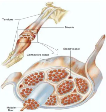
Skeletal muscles represents 40-45% of the body mass and are made of a great quantity of muscle fibers. In adults, the diameter of a muscle fiber ranges between 10 to 100 µm and its length can reach 20 cm. Those muscles are attached to the skeleton by tendons which are connective tissues made of bundles of collagen fibers. Generally, muscle fibers are shorter than the length of a muscle but in some muscles, fibers extend throughout the entire length of the muscle. Figure 2.3 illustrates components of the biceps brachii (BB) with its tendons.

Figure 2.3: Illustration of the biceps brachii with its proximal tendon (at the shoulder level) and its distal one below the elbow joint. Connective tissues are enveloping the muscle as a whole, enveloping groups of muscles called fascicles (as the one shown in front of others) and enveloping each muscle fiber individually within a fascicle (from Vander et al. “Human Physiology: The Mechanism of Body Function”, edition 8th, p.293) [6].

(22)

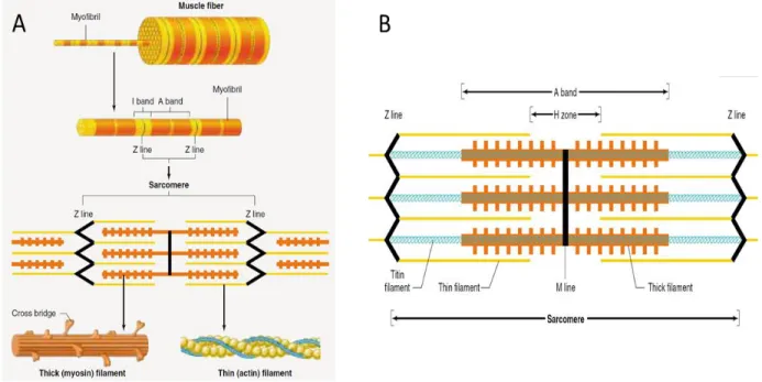
A muscle fiber is made of many cylindrical bundles, named myofibrils, extending all along the fiber length and fused within the tendons of the muscle. Myofibrils present repeating regular zones of black vertical lines separated by pale and darker zones which are shown as yellow and red in Figure 2.4A, The structure between 2 black vertical lines constitutes a sarcomere the length of which is 2-3 µm at rest. A myofibril is thus composed of many sarcomeres in series. The sarcomere pattern is due to 2 kinds of filaments: thick ones called myosin and thin ones called actin. The thick filaments are situated in the centre of every sarcomere with a parallel arrangement which leads to a dark and wide band called A-band. As shown in Figure 2.4B, the thin filaments are located at each end of a sarcomere. One end of the thin filaments is anchored to an interconnecting protein network known as Z-line. The I-band, crossed by the Z-line, includes the thin filaments located at the ends of the A-bands of the two neighbouring sarcomeres. There are also two additional bands: the H-zone is a tiny band located in the middle of the A-band while the M-line is a tiny and dark band located in the middle of the H-zone. Every thick filament is bounded with six thin filaments as a hexagonal array and also every thin filament is bounded with three thick filaments as a triangular shape.

Figure 2.4: A: Structure of a muscle fiber B: Different bands of one sarcomere (from Vander et al. “Human Physiology: The Mechanism of Body Function” edition 8th_{, p. 295).}

(23)

A contraction in a fiber occurs when in each of its sarcomeres, the thick and thin filaments move along each other (Figure 2.5A). This occurs when there is interaction between the many cross-bridges present over the surface of a thick myosin filament interact with a thin myosin filament (Figure 2.5B), each cross-bridge has a tail made of two heads which lengthen out to bind with actin. While an action potential (AP) travels along a muscle fiber, it also penetrates within the fiber through the release of Ca++ ions which are stored in the sarcoplasmic reticulum Figure 2.5C & D). With the presence of Ca++ ions, binding sites on the actin filaments are liberated permitting an interaction between actin and myosin (Figure 2.6). With the energy liberated by the ATP molecules, a sliding movement occurs between actin and myosin and each sarcomere length is reduced. The muscle shortening results from the many individual sarcomere contraction. After the passage of an AP, the Ca++ ions are pumped back in the sarcoplasmic reticulum and the sarcomere length gets back to its relaxed length.

Figure 2.5: A: Sarcomeres in a relaxed condition (upper part) and in a contracted state (lower part). Contraction is associated to a shortening of the H-zone and the I-band occurs while the thick or the thin filaments keep their original length. B: The thick myosin contains many cross-bridges (upper part). The 2 heads of a myosin cross-bridge which can interact with actin (lower part) C: Illustration of the sarcoplasmic reticulum and transverse tubules with myofibrils. D: Perspective view of the transverse tubules and sarcoplasmic reticulum in a single skeletal-muscle fiber (from Vander et al. “Human Physiology: The Mechanism of Body Function” edition 8th_{, p. p. 298, 299,303).}

(24)

Figure 2.6: Contraction of a muscle fiber starts when a cross bridge connects to the actin in thin filament (step 1). As for step 2) the cross bridge moves and produces tension in the thin filament. Step 3) the cross bridge detaches from the thin filament. Step 4) the cross bridge obtains energy so that it can attach to the thin filament to start a new cycle (from Vander et al. “Human Physiology: The Mechanism of Body Function” edition 8th_{, p. 300).}

Types of contraction

There are two main types of contraction: isometric and isotonic. An isometric contraction occurs when the muscle’s length is constant as when the tension generated is not enough to lift a given charge. Isotonic contraction happens when the charge is smaller than the generated force, the muscle’s length shortens but the tension produced is constant. Besides those two main conditions, another one is called “eccentric” (lengthening) which occurs while the muscle length is increasing and the load against the muscle is greater than the generated muscle tension (occurs when going down a flight of stairs) [6] while its opposite is called “concentric” contraction which increases

(25)

tension on the muscle while it shortens. This contraction occurs most frequently in a gym when an athlete lifts a weight [7].

Motor units

A motor unit (MU) is an entity constituted by a motoneuron (MN) and all the muscle fibers it innervates (Figure 2.7A). When an AP is triggered in a MN located in the spinal cord, it propagates along it axon toward the periphery where contact is made at the neuromuscular junction (NMJ) of each of its innervated muscle fibers (Figure 2.7B). NMJs are usually located in the middle of each fiber. Depending on its size, a muscle may contain few or many hundreds MUs. Generally, muscle fibers of a MU are dispersed within the muscle (Figure 2.7C).

Types of Muscle Fibers

Muscle fibers are classified by their maximal velocities of shortening during a contraction and by their energy pathways which is: oxidative or glycolytic. Fibers shortening velocity is associated with myosin isozymes which determines their maximal rate of cross-bridge cycling: fast fibers are those having myosin with high ATPase activity while slow fibers are those with a myosin of low ATPase activity. While the rate of cross-bridges cycling in fast fibers is 4 times faster than in slower ones, the force produced by both types of fibers is roughly the same. As for the machinery used for synthesizing ATP, oxidative fibers are surrounded by numerous blood vessels which give them their dark-red color and their ATP production depends on blood flow. As for the glycolytic fibers which are surrounded by few blood vessels, they contain limited amount of myoglobin which gives them a white pale color. Based on these two criteria there are three types of skeletal muscle fibers (Figure 2.7D) and each of them offers marked difference in their ability to resist to muscular fatigue: while slow-oxidative fibers are fatigue resistant the fast-glycolytic fibers are very easily fatigable while fast-oxydative one stand in the middle of the 2 others. In general, the diameter of the glycolytic fibers are much larger than oxidative fibers. In all types of skeletal muscle fibers, the number of thick and thin filaments per unit in cross-section of a muscle is almost the same.

(26)

Figure 2.7: A: a motor unit is composed of a motor neuron and the muscle fibers it innervates through neuromuscular junctions. B: two motor units with their scattered muscle fibers. C: details of a neuromuscular junction where the motor axon terminal is inserted in grooves at the surface of a muscle fiber. D: various fatigue development rate for the 3 different types of muscle fibers. Each vertical lines is the response to a brief tetanic stimulus (from Vander et al. “Human Physiology: The Mechanism of Body Function” edition 8th_{, p. 305, 316).}

Electromyographic (EMG) signal

Various body organs generate electrical signals as for instances, the electroencephalogram (EEG) which is associated to the brain activity of the brain neurons, the electrocardiogram (ECG) which results from the cardiac cells activity and the electromyogram (EMG) which is generated when many muscle fibers are under contraction. All those signals are associated to the movement of ionic charges and to record them, electrodes are used to transform those ionic currents into electronic ones which can be amplified, filtered, digitized and stored before processing. To record EMG activity, intramuscular electrodes are used when information on a local region of a muscle is searched while surface electrode, i.e. electrodes placed over the skin, are more appropriate when a more global information on a given muscle is needed.

(27)

In 1829, Adrian and Bronk were the first to use an intramuscular needle [8]. Such an electrode is made of a hypodermic needle where recording occurs between the cannula and a conducting core (Figure 2.8A). The outer diameter of the cannula ranges between 0.3 to 0.7 mm while the diameter of the core section is generally 0.1 mm. The cannula is made of stainless steel and the core of silver or platinum [8]. As for surface electrodes which are applied directly on the skin over the muscle to be studied, they are usually made of Ag/AgCl pellets (Figure 2.8B) or from metal such as gold (Figure 2.8C). Surface electrodes are much more frequently used than intramuscular ones since they are not invasive, totally painless and there is no risk of infection. In addition, they can be simply used without special expertise and long term recording is possible.

Figure 2.8: A: intramuscular needle electrode [9]. B: surface Ag/AgCl pallets (from: http://cdn.shopify.com/s/files/1/0150/1454/products/2021_medium.jpg?v=1335040383). C: gold cup surface electrode (from: http: //www.mvapmed.com/Catalog/2014-EEG-Web.pdf). D: Fine wire (from: http:// www. Noraxon .com /wp -content/uploads/2015/01/kinesilogical-fine-wire-emg-booklet.pdf).

Compartments in muscles

Within some animals or human muscles, subdivisions known as neuromuscular compartments can be found. In 1953, Cohen [10] stretched a tiny strip of a cat rectus femoris muscle and observed a contraction in that strip but not in the rest of the muscle. When Weeks and English [11] examined the cat lateral gastrocnemius (LG) muscle to determine behaviour of its anatomical organization, an extensive overlap at the spatial distribution of motoneurons (MNs), that innervate its various primary muscle nerve branches), was found. MNs supplying each PMNB were also of considerably

(28)

different sizes. Those supplying proximal compartments were located in the more rostral portions of the LG and they were among the largest in the pool; small MNs innervated the proximal compartments and their number was small. Neurons that mainly supplied the distal compartments were found in the more caudal parts of the pool and their size was either large or small.

Chanaud et al. [12] studied cat hindlimb to determine the roles of the semitendinosus (ST), the tibialis anterior (TA), the biceps femoris (BF) and the tensor fasciae latae (TFL). Using chronic recording techniques, they collected EMG activity from various sites of every muscle during treadmill locomotion, ear scratch and paw shake. In the BF and TFL, separate neuromuscular compartments were shown to contribute to mechanical movements at the hip and knee joints. For the ST and TA during slow-moderate gait speeds, a region with muscle fibers of type I was active. Increasing speed resulted in additional fibers recruitment. Regions of the muscle with many muscle fibers of type II and III units got active at moderate and high gait speeds. Widmer et al. [13] examined the rabbit’s masseter to determine if its compartments were activated differently during different jaw displacements. Fine wire electrodes were inserted in each of the 9 compartments in the right masseter, in some compartments of the left masseter, at two sites of the right digastric and in one on the left one finally one in each right and left pterygoid muscles. Using principal component analysis (PCA), signals from the 16 recording sites were separated in groups containing 3 to 6 EMG signals. A pair-wise comparison was done to compare activities between the 9 masseter compartments. They demonstrated that during jaw movements similar to those made during rhythmic chewing, the rabbit masseter muscle’s compartments were functional. Such activity in the masseter muscle appears to be related to the unique mechanical actions of the compartments which is required during mastication. As for Lucas-Osma and Collazos-Castro [14] who investigated the triceps brachii of the rat, they found for each of its 3 heads, a region within the spinal cord where their innervating MNs were clustered. The long head had the largest motoneuron pool followed by the medial and lateral heads. While MNs of the medial and lateral heads were mainly located in the rostral part of the spinal motor column, those of the long head occupied mainly its caudal part.

In human lower limb, Wakeling [15] investigated the soleus, the lateral (LG) and medial gastrocnemius (MG) activity during cycling on a stationary bicycle. The LG and MG muscle belly

(29)

was divided in 4 quadrants in which a pair of surface electrodes were put. From low cross-correlation values between every raw EMG signal recorded from a pair of electrodes, it was concluded that the different regions of the gastrocnemius was populated by different MUs. Studying the tensor facia latae of ten normal subjects with inserted fine-wire electrodes, Paré et al. [16] demonstrated a functional different role for its anteromedial and posterolateral fibers. Those findings coupled with anatomical dissections they made on 6 cadavers indicated that TFL activity can be explained by their mechanical advantages on the hip: anteromedial fibers had a superior mechanical advantage for hip flexion comparing to the posterolateral fibers while posterolateral ones have a better mechanical benefit for hip abduction and internal rotation. So, near heel-strike during walking, anteromedial fibers were silent while posterolateral ones were active.

At the trunk level, Paton et al. [17] placed six miniature surface electrodes along each segment (compartment) of pectoralis major (PM) and reported that in an isotonic test, they were independently controlled. The most inferior segments of that muscle were activated when the subjects performed shoulder extension action starting from a flexed position. Inversely, the superior segments of PM were activated in shoulder flexion motion. For horizontal flexion of the shoulder joint, the middle segments of the muscle were activated and this was regardless of the degree of the shoulder flexion. In the back, Holtermann et al. [18] found that each of the 4 anatomical subdivisions (compartments) of the trapezus could be individually activated by voluntary command. At the shoulder level, Wickham and Brown ([19], [20], [21]) investigated the human deltoid and from its 7 compartments, it was found that activity of at least 6 of them could be controlled. The compartment’s activation timing and intensity were dependent upon the muscle compartment’s line of action in a given movement. In a given movement, more active muscle compartments can be functionally considered as principal mover.

When Segal et al. [22] studied the hand flexor carpi radialis (FCR), the extensor carpi radialis longus (ECRL) and the lower limb lateral gastrocnemius (LG), they found that the 3 subdivisions (compartments) of the FCR were individually innervated while 2 nerves innervated at least two different ECRL sections that where not identical to its architecture. In the LG, a single nerve divided into two branches which further subdivide to innervate its 3 heads; thus each head may not be innervated by a private nerve branch.

(30)

In the upper limb, Lee et al. [23], investigated 56 fresh cadaveric arms to determine the spatial location of intramuscular motor nerve endings on the biceps brachii (BB) and brachialis muscles. For the BB (Figure 2.9), they found 3 musculocutaneous nerve branching patterns: type I with one main motor branch which divided into two sub-nerve branches to innervate the LH and SH of the BB; type II with two main motor branches where the proximal branch innervates the SH, and distal one innervates the LH; type III, with one main motor branch that divides into two sub-nerve branches which separately innervate LH and SH (type III is a variation of type I).

Figure 2.9: Three types of nerve branch patterns for BB muscle. In Type I, from a main motor nerve, a branch is separated then it is subdivided into two different parts to innervate SH and LH. In Type II, from a main motor nerve two individual nerve branches innervate SH and LS separately. Type III, which is a variation of type I, from a main motor nerve a branch separates and this branch innervates SH and LH individually (from Figure3 of Lee et al., 2010).

From the BB dissection of cadavers Segal [24] found, on the posterior view of the muscle, signs indicating the presence of up to 6 compartments individually innervated by a nerve branch (Figure 2.10). Being interested in the control of upper-limb myoelectric prostheses, capable of many movements such as some mentioned in the following section which needed many control signals to use them, our attention was focused to this muscle.

(31)

Figure 2.10: A: sketch of the posterior view of biceps brachii illustrating the 6 compartments innervated with an individual nerve branch. B: anterior view of the muscle devoid of any sign the compartments (from Segal, 1992).

Conductivity

1

Many sources are presenting conductivity values of the human body’s tissues. On the web, reference [25] is paricularly interesting because a lot of biological tissues are considered with a frequency range varying from Hz to GHz. The conductivities we used in our simulations (Table 2.1), were gathered from Andreuccetti et al. [26] because this database was established with a collection of many references including the often cited Gabriel et al. [27].

(32)

Table 2.1: Conductivity of different tissues of human body in 100 Hz. *includes cephalic, brachial and basilica veins and the brachial artery (from [26]).

Modern myoelectric prostheses

Following an amputation, the main purpose of an upper arm prosthesis is to restore the many movements needed daily and to have the appearance of the missing part. Besides prostheses used only for cosmetic concern, others are capable of producing a various number of movements. The simplest are body-powered: with a harness and cables, shoulder movements are used to move the forearm and open the hook to grasp and hold an object. Durable, their lack of natural appearance is compensated by their easy operation and low cost. For more versatile prostheses a rechargeable battery is used as the source of power to feed onboard electronics and to activate motors to produce movements as illustrated in Figure 2.11A. The socket is adapted to the anatomy of the amputated person. It includes windows where electrodes make contact with the skin over the muscles used to control the prosthesis: a contracted muscle generates and electric signal (EMG) which is processed by the electronic circuits and used to produce a movement. Depending on the contracted muscle, an electrical motor at the elbow level flex or extend the arm while a second motor can be used to rotate clockwise or contraclockwise the artificial hand and a third one is used to close or open it.

On some prostheses, faster movements and more precise movements can be produced when intensity of the muscles contraction can be achieved by the amputee person. With accurate sensors and modern step-motors, even small objects like coins and keys can be grasped with modern

Tissue Conductivity (S/M) Bone 0.02 Muscle 0.26671 Fat 0.02081 Nerve 0.028042 Blood Vessels* 0.27789 Skin 0.0002

(33)

artificial hand as shown in Figure 2.11B. Since motors, battery and electronics are inside the prosthesis, they are heavier than cosmetic or body-powered prostheses and are more expensive. As modern prostheses offer many degrees of freedom (DOF), more control signals are required to take full benefit of their capabilities. [28, 29]. It is why we are aiming at increasing the number of control sites that could be collected over the biceps by activating each of its compartments.

Figure 2.11: A: Illustration of a myoelectric prosthesis where forearm can be flexed and the hand rotated and close to grasp an object when the thumb and the 2 fingers are moved toward each other (from: http://www.rehab.research.va.gov/jour/98/35/3/bonivento.htm#top). B: Myoelectric prosthesis with several degrees of freedom (from: http:// spectrum.ieee.org /biomedical/ bionics/ dean-kamens-luke-arm-prosthesis-readies-for-clinical-trials).

It should be mentioned that commercially available modern upper limb myoelectric prostheses can have many degrees of freedom and produce many useful hand movements with high accuracy as can be seen in the following web pages:

 www.ottobock.ca  www.touchbionics.com

 www.rslsteeper.com

 www.liberatingtech.com

(34)

Direct and indirect model

In many situations, there is interest to explain an outside observable phenomena in terms of its internal origins. For instance, studying heart electrical behavior, Okada (1956) [30] proposed a theoretical model capable of reproducing the potential fields over the human trunk. To test his model, he conducted experiments where an eccentric z-oriented current dipole, simulating the heart was located in a finite length cylinder filled with a conducting medium (Figure 2.12). As can be seen in the B panel of that figure, the direct model provided a good fit with experiments data but the model did not converge on the border, at the top and at the bottom of the cylinder.

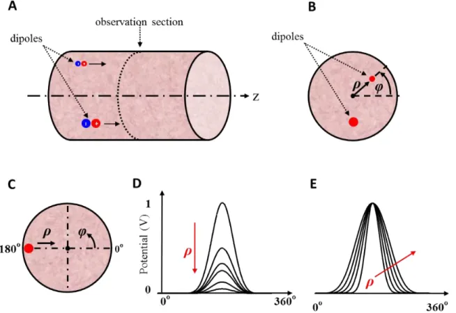
Figure 2.12: A: Cylindrical model of human trunk. The position of the eccentric current dipole was shown as ρ’ and other arbitrary locations can be shown as ρ. B. Comparison of experimental and calculated results. The eccentric z-oriented current dipole is placed along Z-axis at 58.5% of the total height of the cylinder (from: Okada Figs 1 and 2).

This lack of convergence in some conditions for the Okada’s model as well for the model of Frank [31] and the one of Burger et. al [32] was corrected by Lambin and Troquet in 1983 [33]. To get potentials everywhere with a finite cylinder model where the dipole could be oriented everywhere

(35)

in space, they used the Green’s function to solve the Poisson’s equation. Their results for different dipole orientations are shown Figure 2.13.

Figure 2.13: Potentials produced by an eccentric current dipole in a finite length cylinder. The height of cylinder is L= 74.9 cm and its radius is R= 17.8 cm and the dipole is located at 𝝆

′

𝑹 =0.227

and 𝒛 ′

𝑳 = 0.586. The potential unit is arbitrary. A: Curves of potential for 0

◦_{to 180}◦_{(half of the}

surface layer of the cylinder) produced by an eccentric z-orientation current dipole. The small horizontal bars address the zero potential level in each angular curve. B: Curves of equipotential planes for z-oriented dipole C: Curves of equipotential planes for φ-oriented dipole D: Curves of equipotential planes for ρ-oriented dipole (from Lambin and Troquet Figs 2, 3, 5, and 6).

The direct model approach was also used by Saitou et al. in 1999 [34] to calculate over the BB the EMG potentials generated by current sources inside the arm considered as a semi-finite volume conductor. In their experimental results with 3 healthy subjects, 16 pairs of small electrodes were placed over the BB either distally or proximally of the innervation zone (left of Figure 2.14) and low-level isometric contractions were produced in order to be able to record activity of individual MUs. Using the image method and minimizing the differences between experimental results and model data, they estimated the depth and intensity of current sources at the origin of the surface potentials.

(36)

Figure 2.14: Left: 16 pairs of surface electrodes were placed over the BB. Along the fibers direction, electrodes were 5.0 mm apart while across the fibers, the inter-electrode distance was 2.5 mm (Figure3 of Saitou [34]). Right: Illustration of the image method used (from: Figure2 of Saitou [34]).

In their image method (right of Figure 2.14), a dipole represents a current source in the muscular tissue and the dipole is located in the center of the bipolar recording electrodes. In that figure, the Y-axis is perpendicular to the muscle fibers and X-axis is along the muscle fibers direction. Assuming that b ≈ 0, the surface potential is given by their equation 4 which is:

𝛷 = 𝐼 𝑏 2𝜋𝜎[{(𝑋 + 𝑎 2) 2 _{+ 𝑦}2_{+ 𝑑}2_}−3/2_{(𝑋 +}𝑎 2) − {(𝑋 − 𝑎 2) 2_{+ 𝑦}2_{+ 𝑑}2_}−3/2_{(𝑋 −}𝑎 2) ] (1)

where: I (A) = the intensity of the current dipole X (m) =x0 -vt

x0 (m) = the location of the neuromuscular junction in the muscle fiber direction v(m/s) = velocity of the muscle fiber conduction

t(s) = time

σ (S/m) = the conductivity of the medium

a = the distance between the contacts of the bipolar electrode b = the distance between the current sources of a dipole

(37)

X = the coordinate of the direction along the muscle fibers Y = the coordinate of the direction across the muscle fibers

The muscular tissue was considered anisotropic: i.e. 𝜎_𝑥= 0.5 along the fiber and 𝜎_𝑟 = 0.1 perpendicularly to the fiber direction. From Plonsey (1974), the X-axis along the muscle fibers then becomes:

5 X

 

X

(2) The velocity of the muscle fiber conduction was considered to be 4 m/s. The goodness of fit function G to be maximized was:

1 E

G

S

  (3)

where E is the sum of the squared differences between experimental results of surface EMG (𝑀_𝑖𝑗) and calculated results (𝐶_𝑖𝑗) and S is the total power of the experimental records:





16 ₂ 1 1 1 n ij ij j E M C   



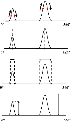
 (4) 𝑆 = ∑16₁₌₁∑𝑛_𝑗=1𝑀_𝑖𝑗2 (5) The numbers of dipoles were increased until G became less than 2% then the number of dipoles at that level was assumed to be optimum. To get more accurate estimation and also to avoid minima, the procedure was repeated 10 times while the initial values of parameters varied randomly. From the 3 subjects, 36 different MUs with different waveforms and distributions were analyzed. Three different types of results are depicted in Figure 2.15 where in each of them, the left-side panels show measured MUAPs while those on the right panels represent calculated MUAPs obtained with the image method. For them, each estimated current source was located at 2.7  1.6 mm deep with 0.5 0.9 nAm in intensity whereas, the total current intensity for a single MU was 2.4  2.9 nAm.

(38)

Figure 2.15: a. MUAP with a single peak and symmetric distribution. b. MUAP with two distinguishable peaks. c: complex MUAP. The dipoles characteristics are shown under each different MUAP (from: Saitou [34] Figs 5, 6, 7).

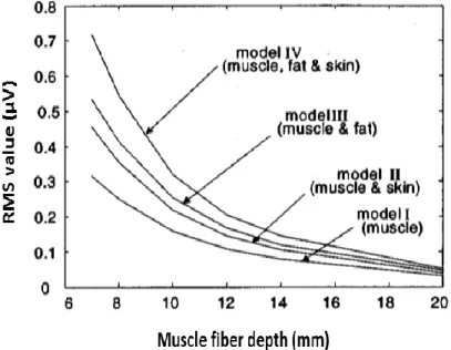
As for Roeleveld et al. [35], they used five different types of volume conductors to investigate the motor unit potentials (MUPs) of the BB. The volume conductor represented by finite/infinite size of cylinders and the number of layers varied as 1, 2 or 3 layers demonstrating muscle, subcutaneous fat and skin. The simulation results of three-layer model was closest to the measured MUPs. The three-layer model is shown in Figure 2.16. The anisotropy condition was taken into account using independent conductivities in radial and axial directions where the radial (𝜌_𝑧) and axial (𝜌_𝑟) conductivity values for muscle tissue were given as 0.1 and 0.5 S/m.

(39)

Figure 2.16: Three-layer model. The radius of muscle, air layer, and thickness of fat and skin were shown by 𝒓_𝒎, 𝒓_𝑨, 𝒅_𝒇 and 𝒅_𝒔 respectively. The MU was positioned as (d) distance inside the model and far from the skin layer. One row of electrodes (A to D) were positioned perpendicular and the other row (1 to 4) was located parallel to the muscle fiber. Inter-electrode distances was set to 12 mm. (from: Roeleveld et al. [35] Figure1).

The fat and skin tissues are considered as isotropic with ρ= 0.05 and 1 S/m respectively. The air medium with zero conductivity and 3 mm thickness surrounded the volume conductor to isolate the model. Based on experimental data the characterization of different models can be found in Table 2.2. The input was given as an arbitrary line source parallel to the skin surface. Two sources were positioned at the ends of the line source to show effects of start and end of the muscle fiber. Two perpendicular rows of electrodes with inter-electrode distances of 12 mm were positioned on the skin surface. One row of the electrodes was located along the muscle fiber and parallel to the skin layer and the second one was situated over the circumference of the model. Potentials were considered relative to a reference electrode (zero potential) located far away from active area. In order to get signals sufficiently higher than noise level during low force contractions, three MUs with different depths (the deepest 15 mm, 7.5 mm and the most superficial 5 mm below the skin layer) were considered. The calculated potentials from these three different depths motor units (Mus) were compared to the experimental recorded potentials which were approximately generated from MUs with the same depth from the skin layer. The results of three MUs along the fiber and perpendicular to the fiber (along the circumference) are shown in Figure 2.17 and Figure 2.18 respectively.

(40)

Table 2.2: Five model configurations (from: Roeleveld et al. [35] Table 1)

Figure 2.17: MUPs along the muscle fibers (1 to 4 refer to electrodes placed along model length in Fig2.16). For the experimental results shown in row 0, 100% of the vertical axis represents the highest value in that condition. Vertical axes in (b) and (c) are relative to the 100% of (a). Simulation results shown in the other rows are from the various models shown in Table 2.2 for a fiber at a specific depth. Amplitude of the maximum simulated result for model III at 5 mm represents 100% on the vertical axis. The % for the other simulated result are relative to that 100% (from: Roeleveld et al. [35] Figure4).

(41)

Figure 2.18: Experimental results (row 0) and simulated ones on the other rows when the electrodes are placed perpendicularly to the muscle fiber (A, B, C, D in Fig. 2.16). The indicated % are relative to the 100% of Fig. 2.17 (from: Roeleveld et al. [35] Figure 5).

As for Chauvet et al. [36], they used an analytical function to localize bioelectric sources from EMG surface recordings. They simulate the generation of 16 surface signals collected at 11 mm intervals over the half cross-section of the upper arm (Figure 2.19). A weak isometric contraction is considered and a single fiber action potential (SFAP) is represented by:

𝑣(𝑡, 𝑟) = 𝑉₂(𝑟) − 𝑏𝑖(𝑟)𝑡2𝑒 −𝑡2

𝜎𝑖(𝑟)

⁄

where t = time, r = electrode to fiber distance, 𝑉2(𝑟)= 2nd phase magnitude, 𝑏𝑖(𝑟) and 𝜎𝑖(𝑟) = shape

coefficients. MUs firing rate depended on the MUAPs duration and ranged between 7 and 33 Hz. To generate a MUAP train (MUAPT), a firing rate was convolved with a MUAP and the resulting EMG signal collected by each electrode represents the summation of the MUAPTs. Signals of 1 s long were generated.

(42)

Figure 2.19: Localisation of emission sources in a muscular cross section. Detection system included 16 surface electrodes over the half part of the upper arm cross section. The (●) symbol is the average geometry of the source found by the proposed program from motor unit action potentials in zone 1, 2 and 4 but in zone 4 it is scattering of micro active area detected on inadequate superimposed SEMGs (from: Chauvet et al. [36] Figure1)

To estimate the electrode-source distance and the sources locations within the model (inverse model), the following equation was used:

𝑉(𝑑, 𝑡) = 𝑘(𝑡)/𝑑𝑎(𝑡)

where 𝑉(𝑑, 𝑡)= amplitude of MUM, 𝑘(𝑡) and 𝑎(𝑡) = middle parameters, 𝑑 = Euclidean distance between the electrode position (𝑥_𝑒, 𝑦_𝑒) and the active source (𝑥_𝑠, 𝑦_𝑠) in the recording system plane. For the optimization method, the gradient method was used where a cost function was minimized:

𝑐 = ∑(𝑌_{𝑖,𝑐𝑎𝑙𝑐𝑢𝑙𝑎𝑡𝑒𝑑}− 𝑌_{𝑖,𝑜𝑏𝑠𝑒𝑟𝑣𝑒𝑑})2 𝑁 𝑖=1 = ∑(𝑎. 𝑋_𝑖+ 𝑏 − 𝑏_{𝑖,𝑜𝑏𝑠𝑒𝑟𝑣𝑒𝑑})2 𝑁 𝑖=𝐼

(43)

and 𝑉_{𝑖,𝑐𝑎𝑙𝑐𝑢𝑙𝑎𝑡𝑒𝑑}, 𝑉_{𝑖,𝑜𝑏𝑠𝑒𝑟𝑣𝑒𝑑} are squares of the calculated and observed amplitude at the ith electrode’s position and at time instant t.

The muscular cross-section is divided in 4 zones (Figure 2.19) and only one active region per zone and per instant is allowed. Two maximum amplitudes for two given distances are initially chosen and the algorithm seeks the electrode with the highest potential value to determine the initial position of the source. With a threshold value for very low amplitude potentials and a stop criteria (< 10% between forward and inverse results), the algorithm iterates along the duration of the signal before displaying the results as in Figure 2.19.

In summary, a model with few simple hypotheses was assumed and simulated signals facilitate the testing of the inverse solution. For zones 1, 2, and 4, the average coordinates of the sources detected were always close to the center where the MUAPs had been placed. As for zone 3, were various MUAPs were superimposed, 3 active regions could be observed but with the algorithm used, their precise location is uncertain. While the arm model appears in Figure 2.19 to be made of 3 concentric layers, there is nothing in the text about them and this model could then be considered as made of a one layer cylinder.

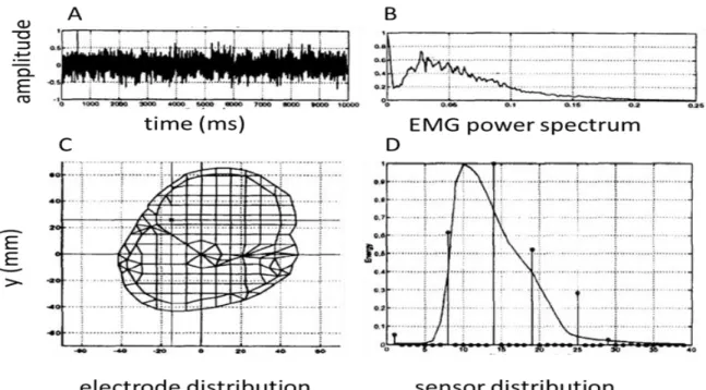
For a more realistic volume conductor, Jessinger et al. [37] used cross-section magnetic resonance images (MRI) of the arm from elbow to shoulder. A finite element model (FEM) was used where bone, muscle and fat tissues with their conductivity was built and Poisson’s equation used for the purpose of identifying a finite number of sources. Experimentally, an array of 4 mm disc electrodes was placed over the bicep and the triceps of the subjects’ left arm. A sample of an EMG signal and its power spectrum are shown in Figure 2.20 A and B. Using a time-frequency distribution for each recorded signal, the frequency of interest was found to be 46 Hz. Assuming a single 46 Hz sinusoidal source, the location of the source was determined with an optimization method. At Figure 2.20 C, the source (small black point) is located within the meshed model. The experimental results and those obtained with the dipole results were compared at Figure 2.20 D.

(44)

Figure 2.20: A: EMG signal; B: power spectrum of the signal C: Estimated source location (small dot) in the upper arm model created from a MRI image. D: Experimental data (vertical lines) compared with simulated results from identified source (from: Jessinger et al. [37] Figure 2).

Figure 2.21 A: The model of volume conductor. Muscle fiber (source) can be situated in the both z and Ө direction of any layers. The detection points can be placed at the boundary of any two layers. Ri (i:1,2) is the radial distance between the source and the center of the volume conductor,

Li (i:1,2) represents the length between the source and the end-plate. Radial distances of different

(45)

A model for surface electromyography (EMG) signal generation in a 4 layers cylindrical volume conductor is proposed by Farina et al. in 2004 [38]. A spatio-temporal function is used to model the generation, spread, and transformation of the axon intracellular action potential (AP) at the end-plate in a muscular (AP) propagating along fibers up to the tendons. The source can be defined either longitudinally (for limb muscles) or radially (for sphincter muscles). Figure 2.21 illustrates geometry of the model in cylindrical coordinates (ρ,Ө,z). The potential distribution over the skin, due to sources in the muscle was obtained with the Poisson equation in the frequency domain where low-pass spatial filters represent the anisotropic muscle tissue and the isotropic fat and skin layers. Results are at the effect that the sub-cutaneous tissue layers increase the detection volume in all directions and reduce its amplitude. To compensate the attenuation and widening of the signal due to the subcutaneous tissue, various recording electrode arrays could be used. The transfer functions of anisotropic muscle tissue and the isotropic layers of fat and skin were proposed.

In 2008, Van den Doel et al. [39] explored the mapping of the activity of individual muscles using surface EMG data from various recording sites which was named computed myography (CMG). The sEMG inverse problem was similar to surface electroencephalogram inverse problem. These sources of potential field are polarization waves know as intracellular action potentials (IAP) initiated at the neuromuscular junction and travelling along the individual muscle fibers. The conduction velocity (~3-5 m/s) is proportional to the radius of the muscle fibers. The motor unit action potential (MUAP) is the signal obtained from a motor unit (MU). The frequency content of surface EMG signals reach up to 500 Hz depending on the electrodes size.

As shown at the left of Figure 2.22, the steps for processing data are:

1) Segmentation of MRI data in order to make a 3D finite element model (FEM).

2) Write 3D volume conduction forward model of muscles to predict the surface voltages. 3) Solve the inverse problem through calculating the most likely current sources that can

(46)

Figure 2.22: Left: The CMG system’s chart. The thick red arrows represent sequential processing steps and the narrow black arrows represent data created or used. The rectangular boxes indicate processes and the skewed boxes indicate data. Right: A 3D domain Ω (including of muscle, fat and bone) with the physical boundary ∂Ω₁ (gray) and the cut boundary ∂Ω₂. (from: Van den Doel et al. [39] Figure1).

The electrostatic potential 𝑢(𝑥) satisfies the generalized Poisson partial differential equation (PDE) on the domain Ω:.

{ −𝛻(𝜎𝛻)𝑢 = 𝐼(𝑥), 𝑖𝑛 Ω, 𝛻𝑛𝑢 = 0, 𝑜𝑛 𝜕𝛺₁, 𝛻𝑛𝑢 = − 𝛴𝑢,𝑜𝑛 𝜕𝛺₁.

Where 𝑛 is the outer-side normal at the boundary and σ(x) is the conductivity tensor which is non-isotropic in the muscles. I(x), the transmembrane current density is assumed to be proportional to the second spatial derivative of the muscle fiber intracellular action potential 𝑉(𝑥, 𝑡).travelling in the muscle fiber direction. At the right of Figure 2.22 (as in the formulas above), there are two types of boundaries: the 𝜕𝛺₁ term is the physical boundary which denotes the skin over the muscle where measurements can be done and the 𝜕𝛺2 term is cut boundary which represents artificial