1 2 3
Characteristics of Mars UV dayglow emissions from atomic oxygen
4
at 130.4 and 135.6 nm:
5
MAVEN/IUVS limb observations and modeling
6 7 8
B. Ritter1,2,*, J.-C. Gérard1, L. Gkouvelis1, B. Hubert1, S. K. Jain3, N. M. Schneider3 9
10
1 LPAP, STAR Institute, Université de Liège, Belgium 11
2 Royal Observatory of Belgium, Brussels, Belgium 12
3 LASP, University of Colorado, USA 13
14
* Corresponding author: Birgit Ritter (b.ritter@uliege.be) 15 16 17 May 2019 18 19 20 21 Keypoints 22
1. Two Martian years of UV dayglow limb observations of oxygen at 130.4 and 135.6 23
nm; first published results at 135.6 nm since Mariner 6/7. 24
2. Solar flux cannot fully explain the brightness variations; strong correlation of the 25
emissions confirms current photochemistry understanding. 26
3. Emissions mainly arise from direct excitation of O; limb brightness and peak altitude 27
are strongly modulated by CO2 absorption. 28
Abstract 30
We present an overview of two Martian years oxygen dayglow limb observations of the 31
ultraviolet (UV) emissions at 130.4 nm and 135.6 nm. The data have been collected with the 32
IUVS instrument on board the MAVEN spacecraft. We use solar flux measurements of EUVM 33
on board MAVEN to remove the solar induced variation and show the variations of the 34
maximum limb brightness and altitude with season, SZA and latitude, which reflects the 35
strong variability of the Martian atmosphere. The 130.4 and 135.6 nm peak brightness and 36
altitudes are strongly correlated and behave similarly. Both emissions are modeled for 37
selected data using Monte Carlo codes to calculate emissions arising from electron impact 38
on O and CO2. Additional radiative transfer calculations are made to analyze the optically 39
thick 130.4 nm emission. Model atmospheres from the Mars Climate Database serve as 40
input. Both simulated limb profiles are in good agreement with the observations despite 41
some deviations. We furthermore show that the observed 130.4 nm brightness is dominated 42
by resonance scattering of the solar multiplet with a contribution (15-20%) by electron 43
impact on O. Over 95% of the excitation at 135.6 nm arises from electron impact on O. 44
Simulations indicate that the limb brightness is dependent on the oxygen and CO2 content, 45
while the peak emission altitude is mainly driven by the CO2 content because of absorption 46
processes. We deduce [O]/[CO2] mixing ratios of 3.1% and 3.0% at 130 km for datasets 47
collected at LS=350° in Martian years 32 and 33. 48 49 50 51 52 53 54 55 56 57 58
1 Introduction
59 60
The lower Martian atmosphere consists mainly of CO2 (e.g. Nier and McElroy, 1977) 61
with minor contributions of argon, N2, O2 and CO. Traces of other species are also present. In 62
the thermosphere, the highly dynamical intermediate region between the lower atmosphere 63
and the induced magnetosphere (Bougher et al., 2000), the composition is also governed by 64
photochemical reactions producing and destroying neutral species and ions. One of them is 65
neutral atomic oxygen that is produced by photodissociation of CO2 (e.g. Barth, 1974) and 66
which supersedes CO2 as the most abundant neutral species above 200 km and up to the 67
lower exosphere. Already since Mariner 4 radio occultation observations in 1965 atomic 68
oxygen is known to be a minor constituent in the lower atmosphere (e.g. Donahue, 1966; 69
McElroy, 1967), where it nevertheless plays a major role in the control of the thermal 70
structure, also in the CO2 dominated region. It contributes to highly efficient cooling of the 71
Martian atmosphere through collisions with CO2 molecules that are hence left in an excited 72
vibrational state and dissipate their energy through the 15-μm thermal emission (Bougher 73
and Roble, 1991, Bougher et al., 2014). 74
75
The first in situ mass spectrometer observations of the Martian atmosphere have 76
been performed by the two Viking landers in 1976 (Nier and McElroy, 1977) that gave insight 77
into the composition of the atmosphere. Quantitative analysis of atomic oxygen could, 78
however, not be performed as oxygen is a highly reactive species and prone to possible 79
recombination with the instrument surfaces. The Neutral Gas and Ion Mass Spectrometer 80
(NGIMS; Mahaffy et al., 2015) onboard the Mars Atmosphere and Volatiles EvolutioN 81
(MAVEN; Jakosky et al., 2015) now performs routine in situ density measurements down to 82
145 km in the atmosphere and even down to about 120 km during ‘Deep Dip’ campaigns of 83
the mission (e.g. Bougher et al., 2017). [O]/[CO2] mixing ratios between 2.2% and 3% at the 84
lowest measured altitudes have been found on the dayside (Stone et al., 2018). Still, the 85
derived oxygen densities have an uncertainty of a factor of 2 due to surface recombination 86
processes (Fox et al., 2017). Oxygen densities have also been derived by photochemical 87
equilibrium calculations using observations of O+ from Viking measurements and electron 88
temperature and density profiles. Hanson et al. (1977) derive an O mixing ratio of 1.5% at 89
130 km. Based on photochemical equilibrium calculations of CO2+, Fox and Dalgarno (1979) 90
find ratios of 1.4% at 120 km and 3% at 130 km. Fox et al. (2017) compare an updated model 91
with NGIMS ‘Deep Dip’ measurements and find model-derived atomic oxygen densities 92
larger by a factor of 4 compared to the mass spectrometer results below 155 km. They use 93
photochemical equilibrium calculations of O2+ and state that their model’s main uncertainty 94
is the electron density. 95
96
In contrast to in situ observations with mass spectrometers, observation of airglow of 97
the respective atmospheric constituents with imaging spectrometers is a powerful tool to 98
probe the atmosphere of a planet with a significant better coverage and down to lower 99
altitudes. Limb observation of airglow emissions is a standard technique to study altitude 100
profiles of the chemical species in the atmosphere and its thermal structures and allow 101
observations at altitudes below the spacecraft periapsis. Emissions from excited O(1S), O(3S) 102
and O(5S) states of atomic oxygen fall into the ultraviolet (UV) range of the dayglow emission 103
spectrum at 297.2, 130.4 and 135.6 nm respectively. While the O(1S) state is largely 104
produced by CO2 dissociation and an exclusive indicator of the CO2 density in the lower 105
thermosphere (~70 km; Gkouvelis et al., 2018), the O(3S) and O(5S) state are expected to be 106
good proxies of the oxygen content in the thermosphere (Strickland et al., 1972; Stewart et 107
al., 1992). Limb profiles from the latter two excited states show peak brightness in the 108
thermosphere between 100 and 150 km. 109
110
The first observations of the 130.4 and 135.6 nm multiplets were performed with UV 111
spectrometers during the Mariner 6 and 7 flybys in 1969 and analyzed by Barth (1971), 112
Thomas (1971), Stewart (1972) and Strickland et al. (1972). They found that resonance 113
scattering of the solar multiplet is the main contributor to the 130.4 nm resonance triplet 114
and that the 135.6 nm line doublet is mainly produced by photodissociation of CO2, while 115
Thomas (1971) concluded that it is mainly produced by photoelectron impact on atomic 116
oxygen. They furthermore indicate that oxygen densities can be directly derived from the 117
130.4 nm data under the assumption of a given exospheric temperature plus a given solar 118
flux at 130.4 nm and derived atomic oxygen mixing ratio of 0.5 to 1% at 135 km. To our 119
knowledge, these are also the only reported results of 135.6 nm observations in the Martian 120
atmosphere up to now. Afterwards, observations at 130.4 nm were reported also from 121
Mariner 9 (Strickland et al., 1973; Barth, 1974) that orbited Mars from November 1971 until 122
October 1972. From these data, Strickland et al. (1973) deduced oxygen mixing ratios 123
between 0.5 and 1% at 135 km. From the comparison of all Mariner data they expect that a 124
variation of the oxygen density by a factor of 3 or more is not unexpected. 125
The UV channel of the SPICAM instrument on board Mars Express observed Mars 126
between 2004 and 2011 and detected the weak signature at 135.6 nm, but no analysis was 127
published. Leblanc et al. (2006) reported a dependence of the 130.4 nm triplet brightness 128
and therefore of the oxygen density on the solar zenith angle (SZA), indicating a drop of 129
oxygen density in the Martian atmosphere by an order of magnitude from SZA interval 14°-130
37° to 37°-60°. Chaufray et al. (2009) reported a decrease in the oxygen density by a factor 131
of 2 between the SZA intervals 20°-55° and 55°-90° from SPICAM observations. Furthermore, 132
they deduced an oxygen mixing ratio between 0.6 and 1.2%. 133
134
With the arrival of the Mars Atmosphere and Volatile EvolutioN (MAVEN) spacecraft 135
at Mars in 2014 a new era of quasi-continuous airglow observations has begun. At the time 136
of writing, two full Martian years of data are available covering a large part of the declining 137
phase of solar cycle 24. The observations encompass various ranges of latitudes and SZA for 138
the different epochs, providing a much more complete picture of the behavior of the 139
planet’s atmosphere than ever before. Among other scientific instruments, MAVEN carries 140
the Imaging Ultraviolet Spectrograph (IUVS, McClintock et al., 2015) that collects spectra in 141
in the range of 120-340 nm, and the Extreme Ultraviolet Monitor (EUVM, Eparvier et al., 142
2015). For the first time, the EUV solar flux is observed while UV dayglow measurements are 143
being taken, which are driven by the solar flux. Chaufray et al. (2015) presented first results 144
of 130.4 nm line limb observations from IUVS and used the data to derive atomic oxygen 145
density in the range of 107–108 cm-3 for temperatures of 200–300 K at an altitude of 200 km 146
using radiative transfer modeling. 147
In the present study, we investigate dayglow limb observations of the oxygen FUV 148
emission multiplets at 130.4 and 135.6 nm by the IUVS instrument and take advantage of 149
the simultaneous observations of the solar input by EUVM. The limb dayside observations 150
range from LS = 217° in Martian Year (MY) 32 to LS = 192° in MY 34. Due to MAVEN’s orbit 151
around Mars and alternating operational modes, there is not continuous coverage of the 152
dayside and neither continuous limb observations, but IUVS still provides an unprecedented 153
and extremely rich dataset. 154
155
1.1 Emissions from the O(
3S) and O(
5S) excited states
156
The OI 3S0–3P transition is an allowed triplet-triplet transition to the ground state 157
emitting at 130.22, 130.49 and 130.60 nm (here referred to as the 130.4 nm line). As it is an 158
allowed transition to the 3P ground state, it is subject to strong resonance scattering, and in 159
particular the solar 130.4 nm triplet radiation is efficiently scattered (Equation (1)). Hence, 160
the Martian atmosphere is optically thick at this wavelength, which requires the use of 161
radiative transfer codes to account for multiple scattering in order to interpret the 162
observations and link its brightness to the O abundance. Apart from solar irradiation, the 163
O(3S) state can be excited by direct electron impact on oxygen atoms (Equation (2)) and by 164
electron dissociation of CO2 (Equation (3)), CO and O2 that leave a neutral oxygen atom in 165
the excited state. Resonance scattering is clearly identified as the major contributor to this 166
emission and other sources play a less important role. Electron impact on CO and especially 167
on O2 can be totally neglected. Even though electron impact on O and CO2 are often 168
neglected as minor sources, these sources now appear to contribute about 15-20% to the 169
total observed emission rate as will be shown in this study. From those two process, electron 170
impact on O is the dominant source above ~110 km. Quenching processes plays no role, as 171
the radiative lifetime of the upper level of the transition is very short, in the order of 10-8 s. 172 hν130.4 + O -> O(3S) (1) 173 e- + O -> O(3S) + e- (2) 174 e- + CO2 -> CO + O(3S) + e- (3) 175 176
The OI 5S0–3P transition is a forbidden quintet-triplet transition to the ground state at 177
135.56 and 135.85 nm (referred to as 135.6 nm line) and features no resonance scattering. It 178
can be considered optically thin at Mars. The transition is weakly metastable (185 μs, Mason 179
1990) and therefore does not experience significant quenching at the low pressure levels of 180
the Martian thermosphere. Possible sources are the same as at 130.4 nm, except for 181
resonance scattering of the solar radiation: electron impact on O (Equation (4)) and electron 182
dissociation of CO2 (Equation (5)), CO and O2. We will show that – following an update of 183
excitation cross sections and modeling – the major source for this emission is indeed 184
photoelectron impact on O while dissociative excitation of CO2 by electron impact remains a 185
minor source. Electron impact on CO and O2 are neglected. Therefore, the produced 135.6 186
nm emission should be a direct indicator of the oxygen density in the Martian 187 thermosphere. 188 e- + O -> O(5S) + e- (4) 189 e- + CO2 -> CO + O(5S) + e- (5) 190 191
Photodissociation of CO2 and CO by EUV solar radiation can lead to the production of 192
oxygen atoms in the O(3S) and O(5S) excited states, but their contribution are expected to be 193
negligible. Only upper limits of cross sections for the production of O(3S) are known that are 194
in the order of 10-20 cm2 at short wavelengths (Gentieu and Mentall, 1973). 195
Figure 1(a) shows a spectrum of the FUV channel of IUVS featuring the oxygen 196
emissions. Other prominent features in the figure are for example the dominant Lyman-α 197
line at 121.6 nm, atomic carbon lines at 127.8, 156.1 and 165.7 nm, a CII line at 133.5 nm 198
and several lines of the CO 4th Positive bands. A more complete list can be found e.g. in 199
Ajello et al. (2019). Figure 1(b) displays the corresponding limb profiles of the 130.4 nm 200
(blue) and 135.6 nm (red) emissions. The dots indicate the maximum brightness of each 201 profile. 202 203
2 Observations
204The MAVEN spacecraft (Jakosky et al., 2015) orbits Mars on a highly elliptic trajectory 205
in a 4.5-hour near-polar orbit with an inclination of 75°. The apoapsis altitude is 6250 km and 206
the periapsis altitude flybys ~160 km. IUVS is one of the eight scientific instruments on board 207 the spacecraft. 208 209
2.1 IUVS observations
210IUVS on board MAVEN is capable of observing the Martian upper atmosphere within 211
a total spectral range of 115–340 nm. This spectral range is divided into a far- and a mid-212
ultraviolet (FUV and MUV) channel. The oxygen emissions at 130.4 and 135.5 nm fall into the 213
range of the FUV channel. The uncertainty of the absolute calibration in the FUV channel is 214
currently estimated to ±25% (Jain et al., 2015). The spectral resolution of the FUV channel is 215
a0.6 nm, therefore the two oxygen multiplets are not resolved in this instrument mode. The 216
echelle channel of IUVS is in principle able to separate the components in the two multiplets 217
and the study of the individual line components will be exciting future work. 218
IUVS operates in limb, coronal scan, and disc modes, depending on the orbital phase. 219
Here, we consider limb observations that cover tangent point (TP) altitudes between 70 and 220
200 km. The instrument is located on a two-axes gimbal and is equipped with a pivoting 221
plane mirror that allows scanning and mapping as well as to chose between two different 222
fields of regard (‘limb’ and ‘nadir’). The combination of those allows the instrument to 223
observe with a duty cycle of 50-100%, even though the respective spacecraft pointing 224
requirements of the other instruments onboard MAVEN are normally not compatible with 225
each other. The entrance slit of the instrument is 11° × 0.06° providing thereby the 226
instrument field of view. The IUVS array detectors record images that contain spatial 227
information in one and spectral information in the other dimension. In limb mode, the 228
entrance slit is parallel to the orbit plane and to the direction of the spacecraft motion. The 229
mirror reflects the incoming UV light onto the detectors before it rotates to point the field of 230
regard to a different tangent point altitude in order to record the next spectral-spatial 231
image. One periapsis limb scan is normally built up of 21 of these images and up to 12 232
individual limb scans can be taken per orbit. The cadence of the observations in limb mode is 233
4.8 seconds, with the integration and read-out time being of 4.2 and 0.6 seconds, 234
respectively. 235
The IUVS instrumental team provides different levels of data products on the NASA 236
Planetary Data System (PDS): Level 1A (raw data), level 1B (calibrated data), and level 1C 237
(processed data). The processed data provides calibrated brightness of individual emission 238
lines that are obtained through multiple linear regression fits of individual spectral 239
components that had been identified in laboratory spectra and taking into account the 240
reflected solar spectrum background (Stevens et al., 2011). The level 1C radiances are 241
binned onto a defined TP altitude grid with a vertical resolution of 5 km. The IUVS FUV 242
spectrum shown in Figure 1(a) is the average of 19 individual limb observations, recorded 243
with tangent point altitudes between 120-140 km above the Martian surface. 244
2.2 EUVM observations
246
EUVM on board MAVEN continuously measures the solar EUV flux at Mars using 247
three different wavelength channels: 0-7 nm, 17-22 nm, and 117-125 nm. From this data the 248
full solar EUV spectrum is reconstructed (Thiemann et al., 2017) and 1 nm resolution spectra 249
from 0-190 nm are available on the NASA PDS, for each minute as well as daily averaged 250
spectra. The total solar 130.4 nm triplet radiance can be extracted from these spectra under 251
some assumptions and can be employed for modeling (Section 4). We use EUVM model data 252
Version 11. 253
254
2.3 Description of IUVS dataset
255
At the time of writing, the observations cover almost two full Martian years and 256
provide an unprecedented dataset, covering various latitude ranges per epoch. The 257
observations cover the time period from October 2014 till June 2018 corresponding to 258
Southern summer in MY 32 till Southern summer of MY 34. The data used in this study is 259
level 1C version 07 and 13. In Figure 1(b) several limb profiles at 130.4 nm (blue) and 135.6 260
nm (red) are plotted. A dot indicates the peak intensity between 100 and 170 km of each 261
profile. In the following, mostly this peak intensity and the corresponding TP altitude (in the 262
following only referred to as altitude) are used for analysis. 263
Note that for the optically thin 135.6 nm profile, the brightness peak altitude is a 264
good approximation for the peak of the actual emission rate, the profile resembles a 265
Chapman layer and the scale heights are relatively small. On the other hand, at 130.4 nm, 266
the atmosphere is optically thick, meaning that the instrument observes the optically thick 267
source function, which is attenuated exponentially by the scattering of the oxygen atoms 268
and also by the absorption of CO2. The observer does not see much farther than a distance 269
corresponding to unity optical depth (τ = 1), hence the observed brightness peak and its 270
altitudes are more spread than at 135.6 nm. Also the topside scale height is significantly 271
larger. The brightness at 135.6 nm is generally lower than at 130.4 nm, but the altitude of 272
the peak emissions is comparable. 273
274
Figure 2 gives an overview of the available periapsis limb dataset observed on the 275
dayside with SZA ≤ 75° and with the condition that at least 6 data points have been recorded 276
within an altitude range of 115-155 km. Additionally, only limb profiles are considered that 277
show an intensity larger than 0.1 kR in both emissions in the peak altitude region. The plot is 278
divided into three different latitude ranges, each covering 60°, for which the maximum 279
intensity of each 130.4 nm limb scan is plotted versus the orbit number. The upper x-axis 280
gives the Martian season in solar longitude LS and the MY. The color code indicates the local 281
time (LT) of the respective scan, binned in 2 hours intervals during daytime and 6 hours 282
intervals for nighttime. Nighttime observations have SZAs below 75° only close to the 283
respective summer pole. Note that not all individual data points are visible due to 284
overlapping. 285
286
The brightness varies significantly throughout the observational period, especially in 287
the first phase of the mission when observed intensities were higher on average than later. 288
The observed variations depend on the season, solar flux, SZA and latitude. We attempt to 289
remove these dependencies in first order in the next paragraph by limiting the SZA range 290
and normalizing the brightness by the solar flux. We will furthermore show the dependence 291
on the SZA for different latitude intervals. The brightness distribution at 135.6 nm looks 292
similar to that of Figure 2 (see supplementary material, Figure S1). 293
294
The peak altitude of the individual scans at 130.4 nm is shown in Figure 3(a). The data 295
are displayed as a histogram due to the altitude resolution of 5 km, which would make it 296
difficult to observe trends in a simple scatter plot. The data is binned into a grid of 5 km 297
altitude versus 100 orbits per pixel. It should be noted that in this figure, all local times and 298
latitudes are included. Nevertheless, a clear variation of the peak altitude with time is seen 299
with altitude minima around Mars apoapsis and maxima around periapsis. The majority of 300
the peak intensity altitudes fall into the range between 115-150 km. The altitude variation at 301
135.6 nm (Figure 3(b)) is very similar, but the 135.6 nm peak emission altitude appears more 302
confined in its distribution. 303
3 Data analysis
305
3.1 Normalization by solar flux
306
Interpretation of previous Martian airglow observations had to rely on solar 307
measurements made close to Earth that required taking into account the relative positions 308
of Mars, Earth and the Sun, the distance of Mars to the Sun and the solar rotation. These 309
factors naturally introduce a varying and possibly large uncertainty. Hence, direct 310
dependences on proxies such as the F10.7 index or using the solar 130.4 nm flux observed 311
from Earth orbit for modeling of the 130.4 nm oxygen line in the Martian atmosphere were 312
possible only to some extent. With the availability of the EUVM instrument in Mars orbit, 313
providing solar flux measurements and extrapolated solar, these uncertainties reduce to 314
instrument calibration uncertainties. In the following, we investigate the direct dependence 315
of the 130.4 and 135.6 nm lines on the solar flux by normalizing the brightness of both 316
emissions by their respective solar forcing. 317
The brightness at 135.6 nm are normalized by the measured EUV flux in the following 318
way: the energy per spectral bin given by the EUVM data is converted to the total number of 319
photons that is able to produce photoelectrons and to furthermore excite the upper state of 320
the O(5S) emission. This includes all wavelengths between 10 nm and 55 nm, which 321
corresponds approximately to the ionization energy of CO2 (13.7 eV) and O (13.6 eV), plus 322
the energy needed to leave the oxygen atom in the O(5S) excited state of 9.14 eV (=135.6 323
nm). The EUV flux below 10 nm has been excluded, as these photons deposit their energy 324
deep in the atmosphere and hence do not have a significant effect on the peak intensities. 325
The 135.6 nm brightness is divided by the resulting number of photons. Additionally, the 326
number of photons in the solar 130.4 nm triplet is calculated from the EUVM measurements. 327
The brightness at 130.4 nm is divided by a weighted combination of the EUV photons (15%) 328
and the solar 130.4 nm photons (85%). The amount of the contribution from each part 329
comes from the model results that are discussed in Section 5. 330
Figure 4(a) shows the maximum brightness of each profile versus the orbit number 331
for all data with SZA < 40°. Blue corresponds to the brightness at 130.4 nm and red to the 332
brightness at 135.6 nm. In Figure 4(b), the brightness is normalized by the solar flux as 333
described above and Figure 4(c) shows the solar 130.4 nm triplet flux in blue, the integrated 334
EUV flux up to 55 nm in red and the distance from Mars to the Sun in black. EUVM 335
observations are continuous, but only data that corresponds to the full IUVS dataset 336
discussed here is plotted. 337
The observational period covers almost the complete descending phase of solar cycle 338
24, as can be seen in the downward trend of the solar flux intensity. This trend is overlaid by 339
the yearly variation due to the changing Mars-Sun distance and, on a smaller scale, the solar 340
rotation. It should be noted that the ratio between the EUV flux shown in the figure and the 341
solar 130.4 nm line flux is not a constant, as the solar spectrum is more variable throughout 342
the solar cycle at shorter wavelength and more constant towards longer wavelengths 343
(Woods et al., 2015). 344
345
The normalization by the solar flux removes some of the variation, for example the 346
highest observed intensities at the beginning of the mission are rather average after 347
normalization. Nevertheless, the resulting intensity distribution is far from being constant 348
and is still surprisingly complex. Strickland et al. (1973) already noted that they could not see 349
a direct correlation between the F10.7 solar activity index and their derived oxygen intensity. 350
Obviously, the atmosphere itself changes significantly with time. Correlation of the 351
brightness at 135.6 nm with the EUV flux shows that 79% of the variation in the brightness 352
can be explained by variation in the solar flux. At 130.4 nm, taking into account 15% of the 353
EUV flux and 85% of the solar 130.4 nm flux, it is 73%. Also interesting is the intensity 354
increase around orbit 5000. It is (i) stronger at 130.4 nm than at 135.6 nm and (ii) even more 355
pronounced after the division by the solar flux. This feature is not related to an SZA 356
dependence or observational bias towards the SZA and coincides with the ending phase of 357
the dust storm period. The approximate same period one MY before, however, does not 358
seem to reproduce this behavior. 359
360
3.2 Correlation of peak intensities and altitudes of 130.4 and 135.6 nm lines
361
As discussed, the excitation of the O(3S) and O(5S) excited states of oxygen are, apart 362
from solar forcing, mainly dependent on the oxygen content in the atmosphere and to some 363
extend on CO2. Hence, a correlation between the intensities of the two corresponding 364
emissions at 130.4 and 135.6 nm can be expected. Figure 5(a) shows the maximum 365
brightness at 135.6 nm versus the brightness at 130.4 nm. A clear correlation is visible, 366
which appears even more confined in Figure 5(b), where the brightness is normalized by the 367
solar flux in the way described above. The corresponding correlation coefficients are 0.8 for 368
the original and 0.75 for the flux-normalized distribution, while the reduced χ2 for a linear fit 369
are 112.7 and 5.5, respectively. The slope of the linear regression curve in panel (a) indicates 370
that the brightness at 130.4 nm is on average more than twice as large as brightness at 135.6 371
nm. 372
When binning the data into 90° LS intervals, this ratio ranges from 0.3 to 0.47 with 373
correlation coefficients between 0.7 and 0.85 (compare Figure S2). The ratio trend follows 374
well the changes in the solar flux at EUV wavelengths below 55 nm and the solar oxygen 375
130.4 nm line. There is no clear dependence on any other parameter like the solar longitude 376
or latitude. A trend with respect to the SZA can be seen in the sense that lower intensity 377
values of both lines are related to higher SZA, as it is expected and shown later. 378
The yellow triangles and blue filled circles represent the datasets that will be 379
discussed in Section 3.4. The triangles are part of the population that is spread-out above 380
the regression curve in Figure 5(a) and move almost exactly onto the curve after flux 381
normalization (Figure 5(b)). During the time of observation of this specific dataset (LS = 350, 382
MY 32), the solar EUV flux was larger compared to the solar 130.4 nm flux than for the blue 383
dataset (LS = 350, MY 33). Hence, the 135.6 nm brightness is enhanced in the MY 32 dataset 384
compared to the later one. 385
Figure 5(c) shows the peak brightness altitude of the two oxygen emissions plotted 386
versus each other in a 5 km binning. The solar flux has no direct influence on the altitude of 387
the peak emission. The peak altitudes at 135.6 nm and at 130.4 nm coincide almost 388
perfectly, the 135.6 nm limb profiles peak appears on average slightly (but less than 5 km) 389
lower than the ones at 130.4 nm. The brightness peaks at about 120 to 125 km. The peak 390
altitude variation at 130.4 nm is larger than the variation at 135.6 nm. No clear correlation is 391
observed between the intensity (non- as well as flux-normalized) and the altitude. 392
393
3.3 Dependence of the peak brightness on the SZA
394
Figure 6 shows the dependence of the solar flux normalized peak brightness at 130.4 395
nm with respect to SZA for three Martian years, MY 32 (blue), MY 33 (black) and MY 34 396
(green). The panels of the figure show in each row latitude intervals of 30° each, going from 397
North to South, and in each column LS intervals of 90°. The plotted data do not distinguish 398
specifically between local times. For a Chapman-like layer like the 135.6 nm emission, a 399
dependence proportional to cos(SZA) is expected, since the photoelectron production 400
decreases linearly with decreasing solar flux. Also, at 130.4 nm a decrease of the brightness 401
with SZA is expected, as because of the optical thickness solar photons can be scattered 402
before reaching large SZA due to the slant atomic oxygen density. Any deviation from this in 403
the flux-normalized data is then due to atmospheric changes. 404
Towards higher latitudes, the drop in intensity with SZA is strongly pronounced. The 405
trend is still visible at lower latitudes, but the distributions are not as confined. This might be 406
an observational bias, as there are more data points within the low latitude datasets. In the 407
following we briefly compare the data taken during the same Martian season but in different 408
Martian years. 409
LS 180°-270°, Northern hemisphere autumn equinox to Northern hemisphere winter 410
solstice: This period includes perihelion at LS = 251° and usually marks the beginning of the 411
dust storm season. There are very few data points for MY 32, but they coincide well with the 412
data from MY 33 in the Northern hemisphere, as well as the MY 33 data coincides well with 413
the data from MY 34 in the Southern hemisphere. In MY 33 at Southern latitudes (30°-60°) 414
two populations are visible that correspond to different local time. The fewer data points 415
with lower intensity that cover a larger SZA range were recorded in the morning, while the 416
other data were taken in the afternoon. This hints to a morning-afternoon asymmetry that 417
was observed by Stewart et al. (1992) in Mariner 9 nadir observations and will be 418
investigated in more detail in a follow-up study. 419
LS 270°-360°, Northern winter solstice to Northern Spring equinox: The flux-420
normalized peak brightness in MY 32 is strongly enhanced compared to their counterparts in 421
MY 33 at equatorial latitudes and SZA around 60°. At the moment, we cannot explain this 422
feature, but it is likely not a true SZA dependence, but rather a localized seasonal effect. This 423
feature is much more pronounced in the non flux-normalized data and corresponds to the 424
Southern summer in MY 32 in the Southern hemisphere close to the equator. While for MY 425
32 the explicit data coverage for this LS interval is from 310° to 350° – and therefore 426
coinciding with observed dust in the atmosphere (Montabone et al., 2015) – the data from 427
MY 33 has been recorded between 340° and 360° solar longitude and does therefore not 428
capture the peak of the dust season, but only parts of its end. Hence, it is likely that this 429
enhancement around SZA = 60° is caused by dust in the atmosphere. It requires, however, 430
further analysis. 431
LS 0°-90°, Northern spring equinox to Northern summer solstice: Again, the earlier 432
dataset (now MY 33) shows higher brightness compared to the following year (MY 34), even 433
though the enhancement is not as strong as for the precedent datasets. Also the increased 434
feature at SZA = 60° is still visible. Intensities within this period are on average slightly higher 435
than in other epochs. 436
LS 90°-180°, Northern summer solstice to Northern autumn equinox: For MY 33 437
mainly the Northern hemisphere is covered by the observations, while for MY 34 more 438
observations have been done in the Southern hemisphere. In the overlapping region close to 439
the equator in the Northern hemisphere, the intensities overlap well, even though the MY 440
34 brightness are slightly lower. 441
442
Note that caution has to be taken when drawing conclusions from this comparison. 443
The LS interval separation might be the same, but the observational coverage within every LS 444
interval is different for different MYs, as has been partly discussed above. 445
446
The behavior of the brightness of the two oxygen lines is very similar, but the 447
dependence on the SZA seems to be less pronounced at 135.6 nm (Figures S3, S4, and S5). 448
Additionally, in certain time periods differences are visible: LS 0°-90° in MY 33: in Southern 449
latitudes, the 130.4 nm intensity decreases strictly and confined with increasing SZA. For the 450
135.6 nm line this behavior can be seen as well, but the scatter is much larger. The same is 451
true for LS 270°-360°, MY 33, where the 130.4 nm brightness shows a strongly confined 452
decrease at high SZAs at the Southern pole region. In contrast, at the same Southern latitude 453
interval, the situation is reversed for the two lines in dataset 180°-270°, MY 33, just before 454
the observations of the previously described dataset. Here, the brightness at 130.4 nm 455
shows a widespread and almost constant behavior towards high SZAs, while the 135.6 nm 456
line follows the expected trends. 457
3.4 Mean profiles
459
The individual limb profiles are quite variable and clearly represent a snapshot of the 460
atmospheric conditions at the time of the observation. In order to provide a more qualitative 461
analysis of the data and to investigate how the atmosphere changes with varying 462
observational parameters, we create mean profiles from several individual limb profiles. A 463
narrow range of observational parameters (LS, SZA, latitude) is selected and all limb profiles 464
corresponding to these conditions are bundled. In the following, we present two example 465
datasets falling into the end of MY 32 (triangles, Figure 5) and MY 33 (filled circles), both at 466
LS = 350° and in the Southern hemisphere at about -16° latitude. They each contain scans 467
with similar SZAs, but cover different local times: in MY 32 the morning is observed while in 468
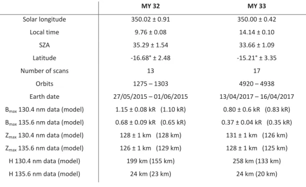
MY 33 the early afternoon is captured. Table 1 gives the overview of the parameters of the 469
two samples. The samples reflect interesting Southern summer conditions, just in the 470
declining phase of the dust storms of the respective year. They have been chosen, as they 471
are one of the few ‘observational condition sets’ that could be found to be very similar for 472
two different MYs. Even though MAVEN/IUVS provides an unprecedented quasi-continuous 473
dataset, and keeps filling in gaps in LS, latitude and SZA, the combination of these three 474
parameters is naturally complex and the same conditions have rarely been caught yet twice 475
throughout the mission. 476
Figure 7 shows the sets of limb profiles for the two MYs, blue lines representing 477
130.4 nm limb profiles, while 135.6 nm limb scans are plotted in red. Top panels refer to MY 478
32, bottom panels to MY 33. The mean of all brightness profiles and the corresponding 479
standard deviation are calculated in every 5 km altitude bin and shown by the black dots and 480
±1-σ horizontal bars. Again, the topside scale heights of the two emissions are notably 481
different and conspicuously larger for the optically thick 130.4 nm triplet (199 km for MY 32 482
and 258 km for MY 33) and small for the optically thin 135.6 nm doublet (24 km for both 483
datasets). The vertical profiles of both lines change significantly from one year to the other, 484
in peak brightness as well as in peak altitude. However, within each dataset the profiles 485
clearly represent a homogeneous group allowing the creation of meaningful average 486
profiles, which will be compared to the corresponding modeling results in Section 5. In order 487
to obtain the peak brightness and altitude with a resolution of 1 km, we fit the vertical 488
profile with a polynomial near the peak altitude following Gkouvelis et al. (2018). The fit 489
results are also listed in Table 1. 490
The 130.4 nm brightness dropped by 30% from MY 32 to MY 33 for the given 491
conditions, while the 135.6 nm brightness decreased by about 45%. As for the peak altitude, 492
the 130.4 nm emission in MY 33 deviates to higher altitudes compared to the previous year, 493
while it remains almost unchanged at 135.6 nm. 494 495
4 Model description
4964.1 Model inputs
497 4.1.1 Model atmospheres 498We use the Mars Climate Database (MCD) Version 5.3 (Millour et al., 2009, 2017) 499
which is based on the LMD model (Forget et al., 1999; Gonzalez-Galindo et al., 2009, 2015) 500
to extract model atmospheres providing the respective altitude distribution of the main 501
neutral constituents, depending on season, local time, latitude and solar activity. At the time 502
of writing, the MCD covers climate conditions for the individual MYs 24–33 accounting for 503
the respective EUV and dust scenarios. The dust scenario properties are based on 504
measurements and modeling (Montabone et al., 2015). 505
Figure 8 shows the density profiles for the atmospheric species related to the oxygen 506
photochemistry (CO2, O, CO and O2) that were extracted from the MCD. The solid lines refer 507
to the conditions of the previously introduced dataset for MY 32 at LS = 350° and the dashed 508
lines to one MY later (second dataset). It is clearly visible that density and temperature 509
profiles, and therefore the density profile scale heights, have decreased as a result of the 510
declining solar cycle. 511
512
4.1.2 Solar flux from EUVM 513
We generate average solar flux EUV spectra from the daily averaged data provided 514
on the NASA PDS. Only dates that correspond to the selected limb profiles are used as input 515
for the models. The solar 130.4 nm line intensity serving as one of the inputs for the 516
radiative transfer code is produced following the same averaging procedure. Since the EUVM 517
data are provided in 1 nm intervals, only a fraction of the solar flux in the interval from 129.5 518
nm to 131.5 nm corresponds to the 130.4 nm multiplet. This fraction is calculated to 0.77 of 519
the full interval, after an estimate based on the high-resolution solar spectrum by the SOHO-520
SUMER instrument (Curdt et al., 2001). We have no knowledge how this fraction might 521
change with time and assume it therefore to be constant. 522
523
4.1.3 Excitation and absorption cross sections 524
Compared to previous studies, some cross sections for the reactions of 525
photoelectrons with atmospheric constituents have been updated. We discuss here briefly 526
which cross sections are used for the calculations. 527
e + O The cross sections for electron impact on oxygen are derived from the 528
analytical formula and parameters given in Green and Stolarski (1972) and Jackman et al. 529
(1977) using the GLOW code (https://www2.hao.ucar.edu/modeling/glow/code). For the 530
130.4 nm triplet, the maximum of the cross section is 17.2 × 10⁻¹⁸ cm2 at an electron energy 531
of 20 eV and in good agreement (within ±10%) with the values from Zipf and Erdman (1985) 532
and Johnson et al. (2003). For the 135.6 nm doublet, we scale the cross section by a factor 533
of 0.78 in order to make it comparable to values from Zipf and Erdman (1985). The 534
maximum cross section at 16 eV results then in 8.9 × 10⁻¹⁸ cm2. 535
e + CO2 For the electron impact on CO2 resulting in 130.4 nm emission, the cross 536
section from Mumma et al. (1972) is adapted with a scaling factor of 0.61 as suggested by 537
Itikawa (2002), resulting in a maximum value of 6.1 × 10⁻¹⁹ cm2 at 115 eV. This value is then 538
in very good agreement with the latest measurements by Ajello et al. (2019), that provide 539
new results at 30 eV and at 100 eV, even though the value at 30 eV is about 30% higher in 540
the Ajello measurement than in the scaled Mumma cross section. The shape of the cross 541
section at 135.6 nm has been measured by Ajello (1971b) and is now rescaled by a factor of 542
0.18, taking into account the measurements by Ajello et al. (2019). The electron impact 543
excitation cross section reaches a maximum value of 1.9 × 10⁻¹⁹ cm2 at 115 eV. 544
e + CO Electron impact on CO resulting in the O(3S) and O(5S) exited states is 545
neglected in the current study as cross sections (Ajello, 1971a) and CO densities are small. 546
The peak cross section for the 130.4 nm triplet at 110 eV amounts to 8.0 × 10⁻¹⁹ cm2 and the 547
cross section for the 135.6 nm doublet is estimated to be smaller by a factor of 0.85 (6.8 × 548
10-19 cm2 at 100 eV). According to Ajello et al. (2019) the cross section for the O(3S) 549
production (130.4 nm) is slightly higher (8.8 × 10⁻¹⁹ cm2 at 100 eV), but even significantly 550
lower for the O(5S) state (135.6 nm): 1.8 × 10⁻¹⁹ cm2 at 100 eV. The values are therefore 551
comparable with the cross sections for electron impact on CO2, but at the respective 552
altitudes between 100 and 150 km, the CO density is at least an order of magnitude smaller 553
than the CO2 density. Also, the contribution by electron impact on CO2 is already a minor 554
source for both oxygen lines, so that the CO-impact source can safely be ignored. 555
e + O2 The cross section for electron impact on O2 is 11.4 times less than the one for 556
electron impact on oxygen for the 130.4 nm line (Stone and Zipf, 1974). The cross section for 557
the 135.6 nm emission is not known, but is most likely even smaller. Furthermore, the O2 558
density is about two orders of magnitude lower than the CO2 density; hence, we neglect this 559
process here for both emissions. 560
Absorption by CO2 During the modeling process, absorption processes due to CO2 561
must be considered. Firstly, the solar flux is accordingly attenuated as it penetrates the 562
Martian atmosphere and secondly, when integrating the emissions from the O(3S) and O(5S) 563
excited states, the CO2 content along the line of sight is taken into account. The CO2 564
absorption cross section is rather large at EUV wavelengths below 100 nm that produce the 565
photoelectrons (in the order of a few 10-17 cm2, Huebner et al., 1992) and the solar flux at 566
these wavelengths is normally fully absorbed at altitudes below 70 km. On the other hand, 567
the CO2 absorption cross section values at 130.4 and 135.6 nm are small. Still, they 568
contribute significantly to the characteristics of the observed limb profile (Section 5.1). At 569
these wavelengths, the high resolution cross sections from Venot et al. (2018) at 150 K are 570
being used: 1.14 × 10⁻¹⁸ cm2 (130.22 nm), 6.77 × 10⁻¹⁹ cm2 (130.49 nm), 5.93 × 10⁻¹⁹ cm2 571
(130.60 nm), 5.3 × 10⁻¹⁹ cm2 (135.56 nm), 8.85 × 10⁻¹⁹ cm2 (135.85 nm). For a cross section of 572
1 × 10-18 cm2 the vertical optical depth for absorption by CO2 becomes unity at 105 km. 573
574
4.2 Models
575
4.2.1 Monte Carlo code 576
Monte Carlo simulation for the calculation of the photoelectron production by the 577
solar EUV flux penetrating the model atmosphere are used in this study. The resulting 578
photoelectron spectrum is a function of altitude between 400 and 60 km above the surface 579
with a spatial resolution of 2 km between 60 and 190 km and 5 km between 190 and 400 580
km. Calculations of the collisional sources are based on the Direct Simulation Monte Carlo 581
(DSMC) method that has been developed to calculate the brightness profiles of emissions of 582
the Earth, Jupiter, Saturn, Venus and Mars atmospheres (Shematovich et al. 2008; Gérard et 583
al., 2008). Collisional excitation rates including photoelectron impact and photodissociation 584
in combination with the respective atmospheric densities are calculated. Finally, the total 585
volume production rates are obtained as a function of altitude, which is integrated along the 586
line of sight to simulate limb observations in the optically thin case. 587
588
4.2.2 Radiative transfer code 589
For the 130.4 nm triplet we combine the photoelectron volume excitation rates of 590
the O(3S) state from the Monte Carlo code with calculations for the production rate from the 591
solar 130.4 nm line. The line shape of the solar triplet is taken from Gladstone (1992) and is 592
normalized using on the reconstructed solar spectra based on the EUVM measurements as 593
described before. For these two sources we employ the REDISTER radiative transfer code 594
from Gladstone (1985) and calculate the effects of multiple scattering including angle-595
averaged partial frequency redistribution. This allows photons to escape an optically thick 596
atmosphere by scattering in frequency from the core of the line into the optically thin line 597
wings. The cascading contribution from upper levels is taken into account by using the 598
‘optically thick’ cross sections from Zipf and Erdman (1985). The population of the ground 599
state sublevels is assumed to be proportional to the degeneracy of the sublevels, i.e. to 2J+1, 600
with J = 2, 1 and 0 for 130.2, 130.5 and 130.6 nm, respectively. This is equivalent to a 601
thermal distribution as shown by Hubert et al. (2015) for the Earth. Furthermore Rayleigh 602
scattering is included with its cross section is derived from the polarizability of the CO2 603
molecule. Instead of using g-factors in the calculations, the scattering of the solar radiation is 604
explicitly taken into account by the radiative transfer code, thus giving internally the primary 605
source of photons due to scattering of the solar flux. The modeling methodology that we use 606
is indeed similar to the one followed by Hubert et al. (2010) for the upper atmosphere of 607
planet Venus, except that we can take advantage of the direct measurement of the solar 608
EUV flux. The resulting optically thick source function, again, is integrated along the line of 609
sight applying the formal solution of radiative transfer in order to obtain limb profiles. The 610
atmosphere becomes optically thick (τ > 1) at the respective line centers (130.2, 130.5 and 611
130.6 nm) below approximately 270, 255 and 215 km (MY 32) and below 240, 225 and 195 612
km (MY 33). At 130 km altitude it reaches an optical depth of τ = 89, 53 and 18 for the 613
atmosphere of MY 32. The corresponding values for MY 33 are τ = 52, 31 and 10. 614
615
5 Modeling the observations
616
In order to better understand how the two oxygen emissions respond to changes in the 617
atmospheric density profiles, the temperature profiles and the solar flux, we perform 618
sensitivity tests. It is understood that the density profiles of the atmospheric constituents 619
and the temperature profile are strongly linked and not independent of each other. Hence, 620
the results of the sensitivity tests should not be interpreted in absolute values, but rather 621
tendencies in the behavior of the observed peak brightness and altitude of the two oxygen 622
multiplets can be derived. 623
624
5.1 Sensitivity to atmospheric constituents
625
For the sensitivity tests, the atmosphere of MY 32 (Figure 8, solid lines) is used and 626
oxygen and CO2 densities are scaled individually, while the densities of all other atmospheric 627
constituents are being kept. These two species are considered to be the dominant 628
contributors to emission and/or absorption of the two lines. Additionally, all atmospheric 629
constituents are scaled with the same factor. The changes in the peak brightness and its 630
altitude are investigated. Figure 9 shows the results. Top panels display the respective peak 631
brightness in kR as a function of the atmospheric scaling factor, while bottom panels show 632
the corresponding dependence of the peak brightness altitude. The red solid line represents 633
the total brightness at 135.6 nm, which is the sum of the electron-impact contribution on O 634
and CO2. The blue dashed-dotted line is the contribution of electron impact on O and CO2 to 635
the 130.4 nm brightness and the dashed line the contribution resulting from the resonance 636
scattering of the solar 130.4 nm flux and subsequent radiative transfer. The solid blue line 637
shows the sum of both contributions. For comparison, the peak brightness and peak 638
brightness altitude of the corresponding mean profile (Figure 7(a,b), Table 1) is added to the 639
plots as data points at scaling factor unity. Note that the ‘steps’ in the altitude dependence 640
of the emission is due to the spatial resolution of the model atmosphere, which is 641
approximately 2 km at these altitudes. 642
643
Oxygen density (Figure 9(a,f)): As expected for an optically thin emission, the 644
brightness at 135.6 nm rises almost linearly with increasing oxygen content. At 130.4 nm, 645
this dependence is much less linear, but it is not as flat as expected for an optically thick 646
emission. This is contrary to the assumption that the 130.4 nm triplet brightness is rather 647
insensitive to the oxygen abundance (e.g. Strickland et al, 1973). The extended optically thin 648
wings of the line triplet are likely to contribute significantly to the brightness at the peak, as 649
has been suggested by Gladstone (1988) for the Earth and by Chaufray et al. (2015) for Mars. 650
At higher altitudes, where the contribution of the optically thick line core is more dominant 651
compared to the wings, the brightness increase with O density increase should be smaller. 652
Notable is also that with increasing oxygen density the photoelectron-impact contribution 653
becomes more important compared to resonance scattering. For the shown example 654
atmosphere, the contribution rises from 18% for no scaling to 33% for a scaling factor of 4. 655
Our understanding is that the solar contribution remains largely determined by the solar flux 656
and is therefore less sensitive to the oxygen density, while the electron-impact excitation 657
rate is proportional to the number of electron-oxygen collisions that occur per second. 658
Hence, increasing the oxygen density increases the primary input of emitted photons into 659
the system, resulting in a near linear dependence. 660
The altitude dependence of both lines is rather flat indicating that the oxygen 661
abundance has almost no influence on the observed peak altitude. This can be also seen 662
implicitly in the 130.4 nm study by Chaufray et al. (2015, Figure 3). Again, the extended 663
optically thin line wings at 130.4 nm could explain the extremely weak dependence on the 664
peak brightness altitude. The slight decrease in altitude at 130.4 nm is most likely owed by 665
the changing importance of the two contributions (resonance scattering and electron 666
impact) whose primary source functions peak at slightly different altitudes, and also by the 667
different scale height of these source functions. This is then smeared out by the radiative 668
transfer, which allows the observer only to penetrate the atmosphere to distances that 669
correspond approximately to where the optical depth becomes unity. These results show 670
also the difficulty and complexity of interpreting optically thick emissions, especially so close 671
to the homopause of the atmosphere. 672
673
CO2 density (Figure 9(b,g)): With increasing CO2 density, the peak brightness of both 674
oxygen emissions decreases. This is (i) due to absorption of the penetrating solar light at EUV 675
and 130.4 nm wavelengths, which results in lower production rates and (ii) because of the 676
absorption at 130.4 and 135.6 nm along the line of sight of the observer. 677
This effect also strongly influences the observed altitude of the peak intensity that 678
increases significantly with increasing CO2 density, since photons produced deep inside of 679
the atmosphere are unable to reach any instrument located at high altitude. The solar flux 680
cannot penetrate as deep into the atmosphere, so that the photoelectrons are produced at 681
higher altitude. The emission is additionally cut on the lower end by the absorption of the 682
denser CO2 atmosphere below. Hence, the altitude of the observed brightness peak can be 683
used as an indicator for the CO2 density rather than the oxygen density. The observed range 684
of peak altitudes (Figure 3) indicates that the CO2 density changes by factors larger than 5 685
within a MY. 686
687
All atmospheric constituents (Figure 9(c,h)): At first glance the combined 688
effects of the changes in the oxygen and CO2 density appear as a superposition of the effects 689
to the peak intensity and altitude as described before. The brightness increases with 690
increasing atmosphere density, but the attenuation by CO2 diminishes the magnitude. The 691
altitude behaves like for the CO2 scaling, as the oxygen density has almost no influence. 692
Caution should be taken when interpreting these results though, as the simple scaling of the 693
atmospheric constituents leads to different changes in the atmosphere, due to the different 694
scale height of O and CO2: both species do not experience the same temperature profile 695
with the same scaling factor. Tests with isothermal temperature profiles show, however, 696
that this effect is not very strong. 697
698
5.2 Dependence on the temperature profile
699
The temperature profile of the atmosphere defines the scale height of the vertical O 700
and CO2 density profiles. It is assumed to be isothermal in the exosphere (above ~200 km) 701
and influences the Doppler width in the radiative transfer model that grows with increasing 702
temperature. Chaufray et al. (2009) found an increase in brightness at 130.4 nm with 703
increasing exospheric temperature at high altitudes (above 250 km) and at the same time a 704
decrease at lower altitudes. The temperature profiles below the exobase are rather complex 705
and rapidly changing in the region of the observed peak emission (Figure 8(b)). In order to 706
simplify, we apply isothermal temperature profiles between 150 and 350 K for the sensitivity 707
study. This means running the simulations without changing the density profiles of the 708
atmospheric components, but only modifying the temperature profile to a constant profile 709
of one temperature at a time. This is obviously not ‘physical’ and a change of the 710
temperature profile influences the scale height of the atmospheric constituents (see also 711
discussion on scale height in Section 5.4), but this approach shall only demonstrate general 712
dependencies. The results are shown in Figure 9(d). As reported by Chaufray et al. (2009), 713
the peak brightness at 130.4 nm decreases slightly with increasing temperature, but not at 714
135.6 nm. The peak brightness altitude, however, does not show any change within the 715
tested parameter range and is therefore not displayed. The changes in brightness can be 716
almost neglected compared to the effects of changing atmospheric constituents and also 717
compared to the changes induced by the solar flux variability. 718
719
5.3 Dependence on the solar flux
720
The solar flux at Mars varies over the course of the collected dataset by ±60% for the 721
EUV and a bit less for the solar 130.4 nm line due to the solar cycle and the varying Sun-Mars 722
distance. The dependence of both lines on the solar flux is strictly linear as seen in Figure 723
9(e). The solar flux here is scaled the same for all wavelengths even though we know that 724
the changes in the solar spectrum are wavelength-dependent to some extent. For the 725
example atmosphere, the variations in the solar flux can infer brightness changes as large as 726
±0.4 kR at 135.6 nm and ±0.65 kR at 130.4 nm. This order of magnitude roughly covers the 727
brightness changes observed during the mission up to now. Note, however, that this is 728
without taking into account the effect of the SZA meaning that the changes in the solar flux 729
cannot fully explain the changes in the observed oxygen dayglow brightness. As seen before, 730
it explains about 70-80% of the changes. The resulting variations then, indeed, reflect 731
changes in the atmospheric structure and composition. 732
The solar energy injected into the Martian atmosphere modulates the atmospheric 733
structure (Bougher et al., 2017), but other than that it has no direct influence on the altitude 734
of the observed peak, at least within a reasonable range of variation. A significant 735
modification of the balance between electron-impact sources and the resonance scattering 736
of the solar line source of photons could lead to a modification of the peak altitude at 130.4 737
nm. This, however, would be more likely to happen if the flux scaling were made 738
wavelength-dependent. 739
740
5.4 Modeling individual cases
741
The results of modeling the two datasets shown in Figure 7 are displayed in Figure 742
10. Panel (a) shows the results for the dataset taken in MY 32 and panel (b) for the dataset 743
taken in MY 33. As before, results at 130.4 nm are shown in blue and at 135.6 nm in red. The 744
data is given as filled circles with the 1-σ variation of the respective dataset as horizontal 745
bars. The model result of the total brightness is represented by the solid lines, which is the 746
sum of a main contribution (dashed line) and a minor contribution (dashed-dotted line). At 747
130.4 nm, the major contribution arises from resonance scattering of the 130.4 nm solar flux 748
and the minor contribution results from electron impact on O and CO2. Electron impact on 749
oxygen is by far the dominant source at 135.6 nm with only very little contribution of 750
electron impact on CO2. The modeled and observed peak brightness and altitude results of 751
the model are given in Table 1. 752
753
Peak brightness: At the peak altitude of the model simulations, the contribution of 754
solar flux to the 130.4 nm triplet brightness is 80% for the first dataset (a) and the remaining 755
20% result from photoelectron impact. For the second dataset (b), this ratio is 84% to 16%. 756
The latter ratio has been used for the flux normalization that was discussed earlier. For the 757
peak brightness of the 135.6 nm doublet, electron impact on O contributes 96% for MY 32 758
and 94% for MY 33 of the total emission for both datasets, making the contribution of 759
electron impact on CO2 rather negligible. Except for the 130.4 nm brightness in MY 33 (+4%), 760
the model results seem to slightly underestimate (-5%) the observed brightness. However, 761
given the excitation cross section uncertainties and the combined uncertainty of the 762
absolute calibration of the IUVS detector and the EUVM instrument as well as in the model 763
atmospheres, these results are in excellent agreement and well within the variability of the 764
dataset. 765
Comparing the two datasets, the brightness at 130.4 nm decreases by 30% from MY 766
32 to MY 33 for the given dataset, while at 135.6 nm it drops by about 45%. The ratio of the 767
peak brightness of the two oxygen lines changes from 0.59 to 0.46. The model atmospheres 768
show a 34% decrease in the CO2 density and a 43% decrease in the atomic oxygen density at 769
130 km, which is in good agreement with the calculated intensity changes. Regarding the 770
solar input, the average solar flux between 0–55 nm drops by 39% and the flux in the solar 771
130.4 nm line by 6% with respect to the MY before. 772
773
Peak altitude: For the definition of the altitude grid, IUVS uses the IAU reference 774
ellipsoid with equatorial radius = 3396.19 km and average polar radius = 3376.20 km (NASA 775
PDS) and the MCD was run with a reference radius of 3396 km. The altitudes were then 776
converted to the IAU ellipsoid. For the MY 32 dataset, the observed limb peak altitude at 777
130.4 nm is extremely well reproduced by the model within the uncertainties. The offset is 778
larger for the dataset of MY 33, in which the fitted observed limb profile reaches its 779
maximum about 5 km above the model maximum. The brightness at 135.6 nm peaks in the 780
IUVS observations about 3 km below the model for the first and 3 km above the model for 781
the second dataset. The vertical resolution of the MCD at these altitudes is 2 km. 782
In contrast to the peak brightness, the observed peak altitude is not dependent on 783
the absolute calibration of IUVS and EUVM. It depends on the atmospheric densities and the 784
CO2 absorption cross sections. The cross sections are the same for both model runs. As the 785
optically thin emission at 135.6 nm is easier to interpret, we rely on the oxygen doublet 786
results for a tentative scaling of the atmospheric components in order to match the model to 787
the observations. Note that for this scaling and the derived results, we do not modify the 788
temperature profile of the MCD atmospheres, which would be beyond the scope of this 789
study. The atmospheric densities of the MCD are scaled by a factor of 0.7 in order to match 790
the altitude, and the oxygen density is afterwards increased by a factor of 1.1 in order to 791
match the intensity. These changes lead to a good agreement of the 130.4 nm brightness as 792
well, while the model limb profile will peak 2 km below the IUVS observations. In order to 793
match the peak altitudes for MY 33, an increase in the atmospheric density by 1.5 would be 794
required, with a subsequent increase of the oxygen density by 20%. This will, however, 795
overestimate the brightness at 130.4 to outside the variability of the dataset. 796