Spatially Resolved M-band Emission from Io's Loki Patera-Fizeau Imaging at the 22.8 m LBT

SPATIALLY RESOLVED M-BAND EMISSION FROM IO’S LOKI

PATERA–FIZEAU IMAGING AT THE 22.8 m LBT

Albert Conrad1, Katherine de Kleer2, Jarron Leisenring3, Andrea La Camera4, Carmelo Arcidiacono5, Mario Bertero4, Patrizia Boccacci4, Denis Defrère3, Imke de Pater2, Philip Hinz3, Karl-Heinz Hofmann6,

Martin Kürster7, Julie Rathbun8, Dieter Schertl6, Andy Skemer3, Michael Skrutskie9, John Spencer10, Christian Veillet1, Gerd Weigelt6, and Charles E. Woodward11

1

LBT Observatory, University of Arizona, 933 N. Cherry Ave., Tucson, AZ 85721, USA;aconrad@lbto.org

2

University of California at Berkeley, Berkeley, CA 94720, USA 3

University of Arizona, 1428 E. University Blvd., Tucson, AZ 85721, USA 4

DIBRIS, University of Genoa, Via Dodecaneso 35, I-16146 Genova, Italy 5

INAF-Osservatorio Astronomico di Bologna, via Ranzani 1, I-40127 Bologna, Italy 6

Max Planck Institute for Radio Astronomy, Auf dem Hügel 69, D-53121 Bonn, Germany 7

Max Planck Institute for Astronomy, Königstuhl 17, D-69117 Heidelberg, Germany 8

Planetary Science Institute, 1700 E. Fort Lowell, Tucson, AZ 85719, USA 9

University of Virginia, 530 McCormick Road, Charlottesville, VA 22904, USA 10

Southwest Research Institute, 1050 Walnut Ste. Suite 300, Boulder, CO 80302, USA 11

Minnesota Institute for Astrophysics, 116 Church St., Minneapolis, MN 55455, USA Received 2014 December 8; accepted 2015 March 17; published 2015 April 30

ABSTRACT

The Large Binocular Telescope Interferometer mid-infrared camera, LMIRcam, imaged Io on the night of 2013 December 24 UT and detected strong M-band(4.8 μm) thermal emission arising from Loki Patera. The 22.8 m baseline of the Large Binocular Telescope provides an angular resolution of∼32 mas (∼100 km at Io) resolving the Loki Patera emission into two distinct maxima originating from different regions within Loki’s horseshoe lava lake. This observation is consistent with the presence of a high-temperature source observed in previous studies combined with an independent peak arising from cooling crust from recent resurfacing. The deconvolved images also reveal 15 other emission sites on the visible hemisphere of Io including two previously unidentified hot spots. Key words: instrumentation: adaptive optics – planets and satellites: individual (Io) – planets and satellites: surfaces

1. INTRODUCTION

Io is the most volcanically active body in our solar system owing to the satellite’s small orbital eccentricity driven by the 4:2:1 Laplace resonance with Europa and Ganymede. The resulting tidal heating powers Io’s global volcanism. Despite decades of observation, including spacecraft encounters by Voyager, Galileo, Cassini, and New Horizons, the details of the energyflow from deposition by tidal heating to release through the surface layers remains elusive, including whether the total rate of energy release is stochastic or steady state. The main driving forces for eruptions at different volcanic sites are unknown as is the time variability of the nature of the activity and energy flow at each of these individual sites. Frequent spatially resolved observations of Io’s volcanism at a variety of wavelengths provide the key to better understanding these processes.

This paper presents M-band (4.8 μm) observations of Io obtained with the full aperture of the Large Binocular Telescope and represents the highest angular resolution yet obtained for ground based observations at this mid-infrared wavelength (∼32 mas FWHM)—similar to the resolution obtained at K′-band (2.2 μm) with the 10 m Keck telescopes (de Pater et al.2014a,2014b). While K¢-band observations are

sensitive to blackbody emission with temperatures ∼1000 K, M-band observations probe emission from lower temperature regions(∼500 K) where K′-band has poor response. Combin-ing the two wavelengths, conveniently now at the same spatial resolution, provides a distinction between active high-tempera-ture lavaflows and cooling emplaced flows. Loki Patera is the

only region resolved in the current study and is the focus of this paper. We present here the first published observations of a spatially resolved Loki Patera since the satellite mutual event occultation timing observations of Spencer et al.(1994) as well

as thefirst thermal emission from a single active site on Io that has been directly resolved by an Earth-based telescope. As such, these observations form the start of a new era promising great strides in understanding the thermal emission, style of volcanic eruptions, and driving force(e.g., sulfur, basaltic, or ultramafic volcanism) at individual volcanic sites.

2. FIZEAU IMAGING

The Large Binocular Telescope(Hill et al.2006) represents

the vanguard of a new generation of extremely large telescopes, with two 8.4 m diameter mirrors separated by 14.4 m center-to-center on a common alt-az mount. Adaptive secondary mirrors (Gallieni et al. 2003) on each of the LBT 8.4 m primaries

provide high-order adaptive optics correction yielding >90% Strehl at wavelengths beyond 3μm. The Large Binocular Telescope Interferometer (LBTI; Hinz et al. 2012) collects

light from both primaries and enables the overlap of the diffraction-limited images of the common target of the two 8.4 m mirrors of the LBT. The LBTI also provides pathlength correction between the two primaries to enable interferometric imaging. LBTI thus yields an image with the Young’s double-slit modulation characteristic of the 14.4 m separation of the two primaries across the overlapped 8.4 m diffraction limited point-spread functions (PSFs). Given the common mount of © 2015. The American Astronomical Society. All rights reserved.

the two LBT primaries, this interference occurs across the image plane (Fizeau imaging).

The resulting inteferometric PSF has excellent spatial resolution in the azimuth direction, exploiting the 22.8 m baseline of the complete LBT, while the PSF in the altitude direction is characteristic of the Airy pattern of a single 8.4 m primary. In the altitude direction, the best resolution is determined by this 8.4 m baseline, while best resolution in the azimuth direction is derived from the structure of the sinusoidal Youngʼs double slit pattern and is therefore determined by the 22.8 m baseline. Thus there is about three times better spatial resolution in the telescope’s azimuth direction as compared to elevation. Note that 0″.032, the M-band spatial resolution in the azimuth direction, corresponds to approximately 100 km on the surface of Io at the time of our observation. Parallactic angle rotation places this high resolu-tion fringe direcresolu-tion across different posiresolu-tion angles of an astronomical target ultimately permitting reconstruction of the target with the effective resolution of the full LBT baseline of 22.8 m. From the perspective of classical aperture synthesis, the u–v plane coverage of the LBT aperture is elongated 3:1 in one direction. Parallactic angle rotation rotates this coverage in the u–v plane ultimately filling in most of the spatial frequencies characteristic of a full 22.8 m aperture. In many practical experiments, observational realities limit parallactic angle rotation during an observation (Conrad et al. 2011) and u–v

coverage is incomplete yielding asymmetric synthesized beams. In the case of the observations discussed herein, the parallactic angle range was 60 degrees, whereas∼120 degrees of rotation would provide maximal u–v coverage for the LBT.

3. OBSERVATIONS AND DATA REDUCTION We observed Io for approximately 1 hr on 2013 December 24th, between 07:53 and 08:51 UT with LBTI-LMIRcam (Leisenring et al. 2014). The geocentric distance, heliocentric

distance, and diameter of Io were 4.23, 5.19 AU, and 1″.19, respectively.12Observations of Io were separated into a total of seven nod sequences (Table 1), consisting of 3000 science

frames per nod interleaved with 1000 off-nod background frames. A wide range of parallactic angles(60°) was acquired in order to maximize u–v coverage necessary for reconstructing an image of Io at the full 32 mas spatial resolution. For a measurement of the PSF, we observed a nearby star (see Table2).

Because phase stabilization was not fully operational, coherent combination was accomplished by manually adjusting the path-length difference in open loop while observing the PSF fringes. Due to the short timescales of the phase variations, the science detector frame size was reduced to a 256 × 256 subarray, accommodating a shorter readout time of 17 ms for capturing“lucky Fizeau” fringes.

Science frames were individually sky and dark subtracted using the median combination of corresponding background frames. Reference pixels located at the top and bottom of each frame provided a means of removing the relative offsets between detector output channels caused by time-dependent voltage drifts. A master bad pixel mask was generated by median combining background-subtracted frames for each nod sequence thenflagging locally deviant pixels. Bad pixels were subsequentlyfixed in each frame using the median of adjacent pixels.

Due to the nature of lucky-Fizeau imaging, a limited fraction of frames captured within an observing sequence show well-phased fringes. Between 2% and 5% of the frames at each of the 7 nod positions were well-phased(see columns 7 and 8 of Table1). These frames were combined to produce the seven

cleaned, but otherwise unprocessed, images(see Figure1) that

were used as input for the data analysis steps described in the following sections.

4. LOKI PATERA 4.1. Morphology

In the following sections we describe the image processing steps used to determine the size, shape, and location of the M-band emission features at Loki Patera. We begin in Section

4.1.1with our shape determination from 1D modeling. Then in

Sections 4.1.2, 4.1.3, and4.1.4 we present the deconvolution techniques that were applied to the full disk to precisely locate 16 volcanoes. As described in Section4.1.6, the results of these steps are required later to place our observed features in relation to the lava lake previously observed at visible wavelengths by Voyager. In Section4.1.5we describe the local deconvolution method that we performed specific to Loki Patera. Finally, in Section 4.1.6, results from the local deconvolution, together with the full disk mapping, are combined to produce thefinal result.

4.1.1. Loki Patera’s Shape from 1D Modeling

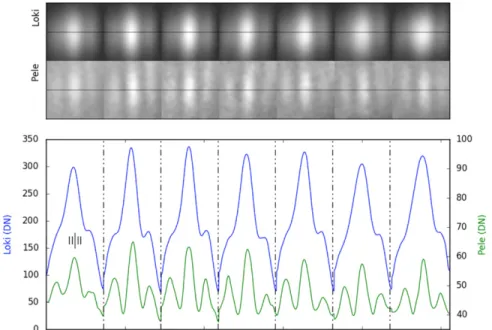
Flux distribution profiles of Loki Patera in each nod are shown in Figure 2. To indicate the achieved resolution, distribution profiles for Pele are also shown in the figure. Because Pele is unresolved, and free of overlapping fringes from nearby emission features, the Pele profiles provide an indication of the contemporaneous PSF. Direct inspection of this unprocessed data clearly demonstrates that the M-band emission at Loki Patera is spatially resolved. The emission is

1 07:53 −0.47 1.022 286.59 −30.0 150 5.0% 2 07:59 −0.37 1.020 287.44 −22.2 138 4.6% 3 08:06 −0.25 1.018 288.43 −15.9 70 2.3% 4 08:13 −0.13 1.016 289.42 −07.5 79 2.6% 5 08:24 +0.05 1.016 290.97 +04.1 94 3.1% 6 08:35 +0.23 1.017 292.53 +16.3 104 3.5% 7 08:47 +0.43 1.021 294.22 +29.1 108 3.6%

Note. Frames were taken with the M-band filter and 17 ms exposure time. 500 frames were taken for a total exposure time of 8.5 s.

12

Ephemeris obtained from JPL’s HORIZONS system: ssd.jpl.nasa.gov/ horizons.cgi.

approximately 3 times the width of the diffraction limited profile seen at Pele and the Loki profile is asymmetrical; i.e., spatially resolved variation in theflux distribution is detectable in these unprocessed data.

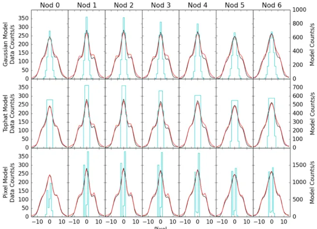
In order to determine the shape of the thermal emission from Loki Patera by an independent method, we fit the 1D cuts through the high-resolution axis of the Loki Patera PSF shown in Figure2with simple 1D models. We tested three models for the shape of Loki Patera’s emission.

(a) Gaussian Model: the brightness distribution is assumed to be Gaussian, centered on Loki Patera. The height and width of the Gaussian are free parameters.

(b) Top Hat Model: the brightness distribution is a pair of top hats both centered on Loki Patera. The widths and brightnesses of both top hats are left as free parameters in the fit, with the restriction that the inner top hat is required to be brighter than the outer.

(c) Pixel Model: the brightness distribution is given a width of six pixels based on the results of the previous models, and each pixel is allowed to vary independently. Each of these models is convolved with the stellar PSF observed on the same night, and the convolved model isfit to the data by a chi-squared minimization routine. We note that the PSF is likely to vary between nods, and we would ideally like to use a simultaneous PSF from a different hot spot in each

image. However, we found that the low signal-to-noise ratio (S/N) of the only other isolated hot spot on the disk introduced significant error into our convolved models, and chose to use the stellar PSF instead.

The results of these model fits are shown in Figure 3. We find that for all seven telescope nods, the best-fit profile is obtained for a model with two emission peaks separated by two pixels with negligible emission from these inner pixels, consistent with the results of the deconvolution discussed below(and shown in Figure5(a)).

4.1.2. Global Deconvolution with Multiple Richardson–Lucy We applied the multiple-image Richardson–Lucy (MRL) algorithm(Bertero & Boccacci2000) to recover a 2D, spatially

resolved flux distribution over the entire disk which is consistent with the measured PSF and the 7 LBTI images. If we denote by g g1, 2,...,gp the detected images (in our case p= 7), by K K1, 2,...,Kpthe corresponding PSFs, and by f the target to be reconstructed, then the iterative algorithm is as follows:

å

where b= 2 is the small background added to the images. The iteration is initialized with a constant array and is stopped after

Figure 1. Unprocessed data (i.e., only “cleaned” as described in Section3) are shown. The first seven images in this panel are of Io; the right-most eighth image is of the PSF star HD-78141. The predominant bright spot is Loki. The Loki image is not saturated and within the linear range of the detector. Several other hotspots are evident even in these raw frames. The images have been stretched to make these evident.

Figure 2. Flux distribution profiles that were used as input for the 1D model fits are shown. The profiles indicated by the blue lines (corresponding to Loki images given in thefirst row of the top panel) are along the higher spatial resolution azimuthal dimension (see Section2) of images. The profiles indicated by the green lines (corresponding to the Pele images given in the second row of the top panel) are similarly along the direction of the high resolution baseline. The width of each panel is 20 pixels(∼215 mas given the detector plate scale of 10.71 ± 0.01 mas per pixel). The width of 4 pixels (∼43 mas) is indicated by the tick mark scale given in the middle of the left hand panel. The two vertical axes give pixel values in data numbers(DN) for Loki on the left, and for Pele on the right.

a suitable number of iterations. The suitable number is determined by visual inspection. In this case, we selected 600 iterations since it provided a reconstruction with the best compromise between blur reduction and noise control. Going beyond this value gives a degraded reconstruction typical of what can occur from over-processing with the RL algorithm. For example, at higher iterations detailed structure appears in the region of Loki that can only be interpreted as an artifact.

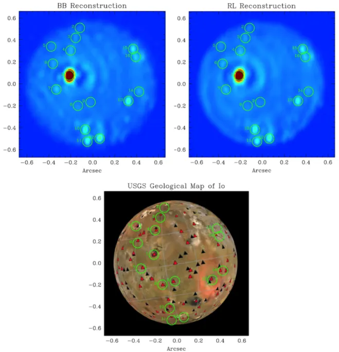
From the reconstruction obtained with 600 iterations it is possible to identify a number of bright spots. In the top right-hand panel of Figure 4 we show the diffraction-limited result where the bright spots identified as volcanoes are indicated with green circles. In the bottom panel of the same figure we show the USGS Geological Map of Io where the identified volcanoes are also indicated (Williams et al.2011).

4.1.3. Global Deconvolution with the BB Method

The Building-Block(BB) method is an iterative multi-frame deconvolution method (Hofmann & Weigelt 1993; Hofmann et al.2005). As a first step, the reduced science images are

de-rotated to correct the parallactic angle changes, centered, and co-added. The result is an image that is the convolution of the target intensity distribution with a co-added sum PSF. Because the LBTI PSFs are also rotated against each other, the coadded PSF is dominated by a bright, almost diffraction-limited core, which appears where the central fringes of all individual rotated point source interferograms cross each other. In an iterative process, delta functions or clusters of delta functions(BBs) are iteratively added to the instantaneous reconstruction in such a

way that the distance between the reconstruction and the observations is minimized. The top left-hand panel presented in Figure 4 shows the diffraction-limited reconstruction of Io using the BB method with a resolution equal to that of a telescope with a circular diameter of 22.8 m. The brightest volcano Loki is surrounded by a patchy dark ring and a bright diffraction ring, which are most likely deconvolution artifacts.

4.1.4. Global Deconvolution with Single Richardson–Lucy (SRL) Both the MRL and the BB methods, described in the previous sections, are effective at producing a single image with S/N at the best possible level for identifying hotspots. However, because the combination process used in these methods does not take into account either deprojection or disk rotation, specific location information is lost in the process. So, for the purposes of mapping we applied traditional SRL (Richardson 1972; Lucy1974) on each of the single epochs.

The SRL iteration uses a simplified version of Equation (1) to

produce seven individual deconvolutions f1,f2,...,f7:

= * * + + f f K g K f b. (2) i k i k iT i i i k ( 1) ( ) ( )

In these images spatial information is preserved. For the mapping step (see Section 4.1.6 below), it is these seven individual deconvolution results that are used. The results described in Sections4.1.2and4.1.3above were used only to confirm that the 16 detections seen in the seven individual SRL results can be trusted. These detections are more easily seen in

Figure 3. The three different 1D models of Loki convolved with the stellar PSF and fit to 1D cuts through the unprocessed emission are shown. The data are shown in black, and the models before and after convolution are shown in cyan and red.

the high S/N results given by those MRL and BB methods. The list of volcanoes and their mapped coordinates are given in Table3.

4.1.5. Local Deconvolution with Multiple Richardson–Lucy and BB In all of the data, both processed and unprocessed, we see a strong emitting region corresponding to Loki. The size of this region is, as seen in the line profiles provided in Figure1, on the order of 3–5 pixels. Given a plate scale of 10.71 ± 0.01 mas per pixel (Leisenring et al.2014), the region is just above the

resolution limit of 32 mas (see Section 2). In situations like

this, deconvolution algorithms can be used to achieve moderate super-resolution (Bertero & Boccacci 2003) and to detect

intensity variations inside the bright region that are only hinted at in the unprocessed data. However, to apply this technique, it

is necessary to remove the strong ringing artifacts surrounding Loki. These artifacts appear in any deconvolved image whenever a strong emitting source is superimposed on an unknown background and the algorithm is asked to reconstruct both the source and the background.

A way for circumventing this difficulty is to extract from the detected images a domain sufficiently broad to contain Loki and sufficiently small to assume that the background, namely the emission of the region around Loki, is approximately constant so that it can be estimated. Thus we extracted from each one of the seven images a square centered on Loki that is 32 pixels wide. As for the MRL case (see Section 4.1.2

Equation (1)), we estimate a background. In this case, from

inspection of the region surrounding Loki, we use b= 48. Moreover, since Loki is not surrounded by empty space we must also correct for possible boundary artifacts. To this

Figure 4. Results from two independent deconvolution methods, BB and RL, shown (top) together with a USGS map of Io (Williams et al.2011) for comparison (bottom). These high S/N results were used primarily to identify the 16 hotspots (see Table3). The apparent difference in the disk flux level that is seen here, as compared to that seen in the individual epochs(see Figure1), is due to the use of a different scale in the two figures: a linear scale in Figure1vs. square root for this figure. The individual epochs from Figure1were used for both the photometry and deprojection steps described in the text.

purpose we use a very simple approach proposed in Anconelli et al.(2006) for multiple image deconvolution. Since the PSFs

are 256 × 256 wide, this step consists of extending by zero padding the local images to 256 × 256 arrays and to apply MRL to these extended images by taking into account the modification of MRL required by the fact that the extended images are zero outside the extracted domains.

The multiple-image MRL algorithm with boundary effect correction is as follows:

å

where the g_j are the 256 × 256 images obtained from the sub-images by zero padding, b is the constant array with all entries equal to 48 as described above, and a is defined as

å

M being the mask which is 1 over the 32 × 32 sub-domains of the 256 × 256 arrays and 0 elsewhere. Since a can take very small values in pixels that are distant from the injected sub-image, a suitable thresholding must be introduced. Details are described in Anconelli et al. (2006).

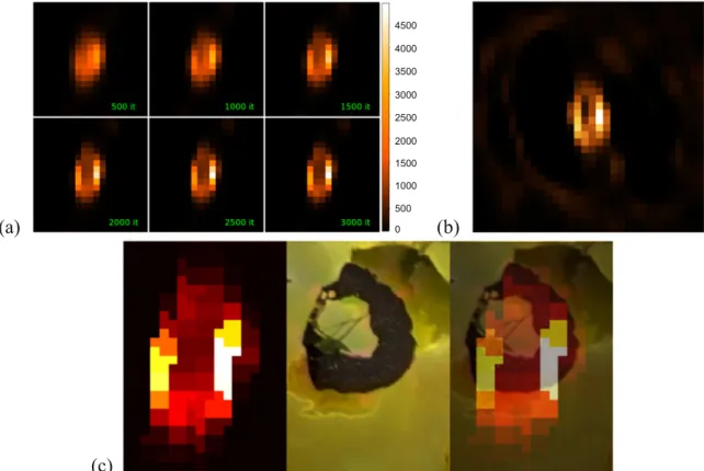
We initialize the algorithm with a constant array and we push the iterations up to 3000. We know that the limit of the iterations consists of a small number of bright spots over a zero background; but we also know that the algorithm is very slow so that this limit is not easily reached. In Figure5panel(a) we show the local Loki reconstruction at six different iteration levels starting with 500 iterations and stepping up in increments of 500–3000 iterations. Some structure appears after 500 iterations and this structure becomes more and more evident with increasing number of iterations.

In Figure5panel(b) we show the Loki image (inner 32 × 32 pixels) reconstructed with the BB method (Hofmann & Weigelt 1993; Hofmann et al. 2005). The applied

preproces-sing of the data was the same as described above, except that we first multiplied the raw images with a circular Gaussian apodization mask (FWHM = 54 pixels) centered on Loki in the first preprocessing step. The BB reconstruction is very

telescope interferometer is a dominant central fringe and two fainter off-axis fringes (side lobes), and not a double peak. If the deconvolution is not perfect (i.e., partial deconvolution), we would also expect to see a central fringe with two fainter side-lobe fringes (fainter than in the unconvolved PSF). Indeed, we see this effect in reconstructions of many of the fainter (low S/N), unresolved volcanoes. In case of a single-peak object, deconvolution artifacts would not lead to a double-peak reconstruction structure, but to a dominant single-double-peak with faint off-axis peaks.

4.1.6. Deprojection and Stitching

We determined the latitude and longitude of the individual hot spots by projecting the SRL deconvolutions of the seven nods onto a rectangular map. Io’s limb is clearly visible in the observations, and the position of the center of the planet in each nod is determined byfitting a circle the size of Io to the limb by eye. Using the sub-observer latitude and longitude of each nod, we projected the image of Io in each nod onto a rectangular latitude-longitude grid at a sampling of two pixels per degree of latitude or longitude.

The maps derived from the seven nods are combined via median-averaging to increase the S/N of the hot spots; the averaged map is shown in Figure6(b). Projecting the data prior

to averaging observations together removes the effects of Io’s rotation, which is necessary to avoid smearing out the hot spots in the averaged images. Latitudes and longitudes for the hot spots were then read off the map and are reported in Table3. Uncertainties are estimated from the brightness distribution of each hot spot in the median-averaged map; smearing in this map is the result of differences in the apparent hot spot position between frames, any inaccuracies in the determination of Io’s center, and the effects of limb viewing. The uncertainties therefore reflect the extent of these three effects. Two of these sources, located in the Colchis Regio, are newly discovered in these data. Given the location of the 2013 August outburst(de Kleer et al.2014a) and the distance of the December sources

from that location, these are possibly hotspots remaining in the aftermath of that event. Figure6(c) shows the surface features

nearest the detected emission that may be the source of the activity.

This technique also gives a crude estimate of the brightness distribution within the Loki Patera feature; a much better estimate is obtained from the local reconstruction, a recon-struction which combines all seven epochs of Loki imaging, discussed in Section 4.1.5, which does not suffer from disk rotation effects because it relies on images centered on Loki Patera. In order to project the local reconstruction of Loki Patera onto a latitude-longitude map, we replaced the central 32 × 32 pixels of the middle nod (#4), which are centered on Loki Patera, with the local reconstruction. This process amounts to placing the pixels in the local reconstruction in their appropriate location on Io’s disk in an unprocessed image, so that we can project this reconstruction onto the same latitude-longitude grid as the other hot spots via limb-fitting. The resultant brightness map of Loki Patera, together with a

(3) Dazhbog +55.0 ± 2.0 302.0 ± 2.0 (4) Amaterasa +42.5 ± 5.0 309.0 ± 3.0 (5) Surt +47.0 ± 2.0 339.0 ± 2.0 (6) Fuchi +26.0 ± 3.0 326.5 ± 3.0 (7) Tol-Ava +00.5 ± 1.5 323.0 ± 4.0 (8) Mihr −18.0 ± 2.0 304.0 ± 2.0 (9) Gibil −16.0 ± 1.5 293.5 ± 1.5 (10) Rarog −40.0 ± 2.0 304.0 ± 2.0 (11) Heno −58.0 ± 2.0 309.0 ± 4.0 (12) Lerna Regio −57.0 ± 3.0 288.0 ± 2.0 (13) Pele −19.5 ± 3.0 245.5 ± 1.5 (14) Pillan −11.0 ± 2.0 242.0 ± 2.0 (15) Colchis Regio 1 +15.5 ± 1.5 229.0 ± 4.0 (16) Colchis Regio 2 +29.5 ± 1.5 230.0 ± 3.0

visible light image of the same region obtained during a Voyager encounter, is shown in Figure 5panel(b).

4.2. Photometry

We measure the radiant flux from Loki Patera by two different methods: by calibrating to a standard star and by calibrating to Io’s disk brightness.

We observed the star HD 78141, which is a K0 star with a WISE Band 2 (4.6 μm) of 5.62 ± 0.05 mag and a WISE Band 1 (3.4 μm) magnitude well-matched to the L-band photometry from Heinze et al.(2010). The WISE fluxes therefore provide an

accurate representation of LMIRcam’s L and M bands, especially given that K0 stars have relatively flat spectra across these wavelengths. Using the values from WISE yields a measured absolute flux for HD 78141 of 1.37 × 10−13W m-2mm−1. We then extract theflux density of Loki Patera by measuring the flux ratio between Loki and the star based on aperture photometry. Background emission from Io’s disk was estimated and removed in two separate ways:(1) estimating the background from regions on Io free of hotspots; (2) taking the median from an annulus placed around Loki Patera. Multiple circular apertures with different radii were generated around Loki with matching aperture placed on the reference star to measure theflux ratio. To account for its extended nature, apertures around Loki Patera were 10% larger than those around the reference star. Wefind a ratio of 1.13± 0.06 between the two, yielding an observed flux for Loki of 1.6 × 10−13W m-2mm−1. Propagating the ratio

uncertainty with that of the stellarflux yields a value of 62 ± 4 GWμm−1str−1for the radiantflux of Loki Patera.

We independently flux-calibrate the Io observations using the brightness of Io’s disk in regions without hot spots. This calibration is not affected by the observing conditions, and relies on the fact that the average reflected sunlight from Io’s disk is stable in time, once solar distance is corrected for. We use a large area of Io’s disk free of hot spots to measure the average background counts per pixel, and scale the entire image so that the flux density per square arcsecond matches that of previous well-calibrated observations.

We then use theflux-calibrated raw (not deconvolved) images to extract theflux density of Loki Patera. We perform aperture photometry on Loki Patera using apertures small enough that they do not overlap with other hot spots on the disk. Such apertures are too small to include the full wings of the PSF, and we estimate and correct for this effect using the PSF from the star observations. Based on applying this extraction to each of the seven nods using a variety of apertures, wefind an M-band flux density of 53± 4 GW μm−1str−1.

If we conservatively estimate that photometric uncertainty is 10%, averaging these two results yields afinal radiant flux of 57.5± 6 GW μm−1str−1.

4.3. Scientific Interpretation

Loki Patera is the most powerful volcano in the solar system, with a total radiated power output of ∼1013 W (Rathbun et al.2004; Veeder et al.2011), 25% of the power output of the

4500 4000 3500 3000 2500 2000 1500 1000 500 0

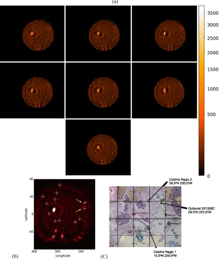
Figure 5. In panel (a), the local Loki reconstructions corresponding to increasing numbers of iterations of the MRL method with boundary effect correction and in panel(b) the BB reconstruction are shown. The apparent shape of Loki is elongated due to the beam shape (i.e., three times better spatial resolution in azimuth vs. elevation). In panel (c) we show three views of the lava lake at Loki Patera: the deconvolution result re-mapped as described in Section4.1.6, the Voyager image, then the two overlaid with one another in thefinal image on the right. The scale on the right side of panel (a) is given in data numbers (DN) and applies to all three panels. The position of the emission feature relative to the lava lake(imaged by Voyager) shown in panel (c) is the best fit to our measurement using the techniques described in the text, however a shift that would put its postion at a point that better matches the dark patera is within the error of our measurement.

Figure 6. Three views of Io. In panel (a) the SRL deconvolutions at each of the seven individual epochs that were used to compute latitudes and longitudes are shown. In panel(b), the global map that was formed by stacking the deprojections of these seven deconvolutions is shown. This is the projection of the observations onto a latitude-longitude grid: the map shown is a median-average of a the projected maps for each nod. The white plus signs indicate the locations of the hot spots tabulated in Table3based on the positions of the associated surface features as observed by spacecraft. Finally, in panel(c), the locations of two hot spots in the Colchis Regio (indicated by yellow arrows in panel (b)), that do not correspond to known hot spots, are shown with respect to other features given on a USGS map of Io (Williams et al.2011). The 2013 outburst location (de Kleer et al.2014a) is also show in panel (c).

Earth. The horseshoe-shaped patera is most likely a crusted-over lava lake (Rathbun et al.2002; Matson et al. 2006). It

exhibits periods of greatly increased near-infrared brightness lasting several months, which were roughly periodic during the 1990s, with a periodicity of about 540 days (Rathbun et al. 2002). However this periodicity did not persist into the

2000s(Rathbun & Spencer2006). The brightenings have been

attributed to waves of resurfacing, in which the lava lake crust is disrupted along a front propagating around the patera, exposing magma which then cools, regenerating the crust (Rathbun et al.2002). The resurfacing waves seem to originate

from the southwest corner of the patera, which has persistently higher temperatures (Howell & Lopes 2007), and propagate

counter-clockwise. An image at 2.2μm taken on UT 2013 August 22 with the Keck telescope (de Pater et al. 2014b)

shows that the brightest high-temperature emission at that time was indeed in the southwest corner of Loki Patera.

Keck and Gemini AO observations in 2013 August and September show that Loki had a 3.8μm brightness of 100–120 GWμm−1str−1at that time, typical of its bright phase(de Kleer et al. 2014a; de Pater et al. 2014a, 2014b). However, it had

faded to <12 GWμm−1str−1by 2013 December 15 (de Kleer et al. 2014b). IRTF Jupiter eclipse/occultation data show that

much of this fading had occurred by 2013 November 1 (Rathbun et al. 2014). Likely the 2013 December 24 LBTI

image was taken shortly after the end of a typical Loki brightening, at a time when the resurfacing wave had completed its counter-clockwise journey from the southwest to the eastern side of the patera. The brightness of Loki Patera at this time was approximately 60 GWμm−1 str−1 (see Section 4.2). A plausible interpretation of the LBTI Loki

image is that we are primarily seeing emission from two sources, the persistent high-temperature source in the southwest corner of the patera, and radiation from the cooling crust generated by the recently ended resurfacing wave, which is brightest on the eastern side of the patera where the wave has most recently passed, and the crust is youngest and warmest. This hypothesis can be tested further with more quantitative analysis of the observations, which is beyond the scope of this paper.

5. CONCLUSION

The resolved views of Loki that we have shown here, the first from ground-based direct imaging, indicate emission from two locations within the patera’s lava lake. The feature seen in the southwest corner is likely a persistent high temperature source, while the one seen in the southeast is likely radiation from nearby cooling crust.

We have shown that the existence of two distinct sources can be seen, not only in the results of 2D image deconvolution via two independent methods, but also from the unprocessed data via simple one-dimensional model fitting techniques. To accurately place the two features with respect to the lava lake, a complete mapping of the full disk was performed and the locations of 15 other eruption sites were located via deprojec-tion. Two of these, in Colchis Regio, are newly discovered

eruption sites that are likely associated with a recent outburst in that area.

The research was partially supported by the National Science Foundation, NSF Grant AST-1313485 to UC Berkeley, and by the National Science Foundation Graduate Research Fellow-ship under Grant DGE-1106400. Development of LMIRCam was supported by NSF grant AST-0705296.

1. The LBTI is funded by the National Aeronautics and Space Administration as part of its Exoplanet Exploration program.

2. The LBT is an international collaboration among institutions in the United States, Italy, and Germany. LBT Corporation partners are: The University of Arizona on behalf of the Arizona university system; Istituto Nazionale di Astrofisica, Italy, LBT Beteiligungsge-sellschaft, Germany, representing the Max-Planck Society, the Astrophysical Institute Potsdam, and Heidel-berg University; The Ohio State University; and The Research Corporation, on behalf of The University of Notre Dame, University of Minnesota, and University of Virginia.

REFERENCES

Anconelli, B., Bertero, M., Boccacci, P., Carbillet, M., & Lantéri, H. 2006, A&A,448, 1217

Bertero, M., & Boccacci, P. 2000,A&AS,147, 323 Bertero, M., & Boccacci, P. 2003,Micron,34, 265

Conrad, A., de Pater, I., Kürster, M., et al. 2011, in Proc. EPSC-DPS, Observing Io at High Resolution from the Ground with LBT,795 de Kleer, K., de Pater, I., Davies, A. G., & Adamkovics, M. 2014a,Icar,

242, 352

de Kleer, K., de Pater, I., & Fitzpatrick, T. 2014b, in AAS/DPS 46, Volcanic Activity on Io: Timelines and Surface Maps,418.13

de Pater, I., Davies, A. G., de Kleer, K., & Adamkovics, M. 2014a, in ESLAB Symp. on Volcanism, ESTEC, Time Evolution of Individual Volcanoes on Io: Janus Patera, Kanehekili Fluctus and Loki Pater

de Pater, I., Davies, A. G., Adamkovics, M., & Ciardi, D. R. 2014b,Icar, 242, 365

Gallieni, D., Anaclerio, E., Lazzarini, P. G., et al. 2003, Proc. SPIE,4839, 765 Heinze, A. N., Hinz, P. M., Sivanandam, S., et al. 2010,ApJ,714, 1551 Hill, J. M., Green, R. F., & Slagle, J. H. 2006, Proc. SPIE,6267 10Y, Hinz, P., Arbo, P., Bailey, V., et al. 2012, Proc. SPIE,8445, 0U

Hofmann, K. H., Driebe, T., Heininger, M., Schertl, D., & Weigelt, G. 2005, A&A,444, 983

Hofmann, K. H., & Weigelt, G. 1993, A&A,444, 328 Howell, R. R., & Lopes, R. M. C. 2007,Icar,186, 448

Leisenring, J. M., Hinz, P. M., Skrutskie, M., et al. 2014, Proc. SPIE,9148, 2S Lucy, L. B. 1974,AJ,79, 745

Matson, D. L., Davies, A. G., Veeder, G. J., et al. 2006,JGRE,111, 9002 Rathbun, J. A., McGrath, C. D., & Spencer, J. R. 2014, LPI,45, 1108 Rathbun, J. A., Spencer, J. R., Davies, A. G., Howel, R. R., & Wilson, L. 2002,

GeoRL,29, 1443

Rathbun, J. A., Spencer, J. R., Tamppari, L. K., et al. 2004,Icar,169, 127 Rathbun, J. A., & Spencer, J. R. 2006,GeoRL,33, 17201

Richardson, W. H. 1972,JOSA,62, 55

Spencer, J. R., Clark, B. E., Toomey, D., Woodney, L. M., & Sinton, W. M. 1994,Icar,107, 195

Veeder, G. J., Davies, A. G., Williams, D. A., et al. 2011,Icar,212, 236 Williams, D. A., Keszthelyi, L. P., Crown, D. A., et al. 2011, Geologic map of

Io: US Geological Survey Scientific Investigations Map 3168, Scale 1:15,000,00025,http://pubs.usgs.gov/sim/3168/