Analytical procedure to derive P-I diagram of a beam under explosion
Lotfi HAMRA Phd candidate University of Liège Liège, BELGIUM [email protected] Jean-François DEMONCEAU Assistant professor University of Liège Liège, BELGIUM [email protected] Vincent DENOEL Associate professor University of Liège Liège, BELGIUM [email protected]Summary
The aim of this paper is to study a beam extracted from a frame and subjected to blast loading. The demand of ductility depends on six dimensionless parameters: two related to the blast loading, two referring to the bending behaviour of the beam and two corresponding to the dynamic behaviour of the rest of the structure. We develop a full analytical procedure that provides the ductility demand as a function of these six dimensionless parameters.
Keywords: analytical procedure; blast loading; membrane force; p-I diagram.
1. Introduction
Recent standards or norms are concerned about the need to confer robustness to structures subjected to exceptional events such as natural catastrophes, explosions or impacts, in order to avoid their progressive collapse.
An accurate finite element modelling of frame structures under explosion is expensive and simpler analysis tools are welcome. A simple model of the system is developed with a condensation of the rest of the structure usually referred to as the Indirectly Affected Part (I.A.P.). In this perspective, this paper focuses on the determination of the required ductility of frame beams subjected to a blast loading considering the effects of lateral inertia and restraint.
In the literature, the conversion of a continuous beam to an equivalent elastic perfectly-plastic single-degree-of-freedom (SDOF) system is suggested in order to develop its corresponding p-I diagram [1]. Some full analytical formulae are proposed to derive the p-I diagram curves [2]. However, the development of internal forces is assumed to be elastic perfectly plastic curve, neglecting any hardening effect such as the development of the membrane action.
Langdon and Schleyer presented a model of a beam subjected to blast loading, including some lateral and rotation restraints at the ends as well as the action of the membrane force [3]. Fallah and Louca proposed to derive a p-I diagram for an equivalent softening or hardening SDOF models substituting the structural behaviour of a corrugated wall by an equivalent bi-linear resistance vs. displacement curve [4].
The aim of this paper is to establish the p-I diagram of a frame beam subjected to a close-field local internal blast loading including the effect of nonlinear membrane action, the bending moment-axial plastic resistance interaction curve of the beam as well as the dynamic interaction with the reduced model of the I.A.P. of the structure. A full analytical iterative procedure is provided depending on six
dimensionless parameters. Fig. 1: (a) Sketch of the considered problem, (b) Idealized
blast loading, (c) Axial force-bending moment interaction law.
2. Problem formulation
2.1 Description of the problemThe main challenge is to develop a full analytical procedure to design a beam extracted from a frame and subjected to blast loading. We considered that the I.A.P. of the structure provides a lateral restraint and inertia to the beam. Moreover, the beam is studied in large displacements and small rotations.
The beam is assumed to be under a uniformly distributed blast loading p(x,t), see Fig. 1. The beam has a length 2l and is characterized by a lineic mass ms, and an equivalent elastic bending stiffness
ks.
Specific to this problem is the lateral restrain K* and the mass M* that materializes a horizontal restraint as well as a participating mass; they model the passive interaction of this beam with the I.A.P. of the structure. The loading is assumed to develop synchronously along the beam and is idealized as a triangular pulse, see Fig. 1, so that
0 1 d t p t p t (1)where t represents the time variable, p0 is the peak blast pressure and td is the positive phase
duration. The momentum I associated with this pressure field is thus given by
0d .
I p t l (2)
This problem has been studied numerically by performing the (p0,I) diagram [5] which gives the
maximum response of the beam for various blast durations and intensities.
Further to the explosion, the bending plastic mechanism is formed and the membrane force rises while the mid-span displacement becomes larger. A general M-N plastic interaction between the bending moment M and the axial force N is introduced in the model
1 pl pl N M M N β α γ (3)
where Mpl and Npl are the plastic bending and axial resistances. Symbols α, β and γ depend on the
shape of the cross-section properties [6]-[7].
Several assumptions are adopted: (i) the lateral restraint remains elastic; (ii) the beam-to-column joints are perfectly rigid; (iii) the axial elongation of the beam is neglected; (iv) the material is elastic-perfectly plastic; (v) the strain rate effect is not considered; (vi) the travelling hinges as well as the shear mode failure are not included in our study; (vii) the analysis is performed in large displacements/small rotations.
2.2 Equations of motion
The equation of motion is obtained by differentiating the energy conservation law with respect to time and dividing by the velocity
2 2 * * , ,K 2 2 4 4 , , s X int b X X X int X l l X XX M M M F F pl (4)where Ms=2msl/3 is the generalized mass corresponding to the assumed kinematics. The equivalent
internal force in the beam, the lateral restraint and the membrane force are respectively given by
int,b ) , , (for 4 (for and 0) s y y X X X F X X X k M N X X X l (5)3 * int,K 2 2 F K X l (6)
2 * * 2 2 2 pl . X X N K M M X X l l X (7)where Xy is the displacement of the beam when the plastic mechanism is formed.
2.3 Scaling and dimensionless formulation
Introducing reference scales, in length Xy and in time T M /s ks (which corresponds to the characteristic period of the elastic beam without lateral restraint and inertia), the dimensionless equation of motion of the structure can be written as
2 2
,b , 2 2 K 1 M M y int , , i tn 1 d y X X XX F X X X F X p τ ψ θ ψ θ τ (8)where X X X / y is the dimensionless displacement, τ=t/T is the dimensionless time, τd=td/T is the
dimensionless loading duration, ψM=4M*/Ms is the ratio of the lateral mass to the mass of the beam,
ψK=K*/ks is the ratio of the lateral restraint to the stiffness of the beam, θy=Xy/l is the yield rotation, 0 / s
p p p is the dimensionless peak overpressure of the blast loading, ps=4Mpl/l² is the static
pressure at which the plastic beam mechanism is formed and,
,b ,b for 1 for 1a , , nd 0 int int s X X m n X X X X X F F p l (9) ,K 2 3 ,K 2 int int K y s F F pl ψ θ X (10)The dimensionless axial force n=N/Npl and its interaction with the dimensionless bending moment
m=M/Mpl are given by:
2 2 4 y X 2 KX M n ξθ ψ ψ X XX (11) 1 mβ γnα (12)where ξ=(Mpl/2l)/Npl is the ratio of bending to axial strengths.
The set of Equations (8), (11) and (12) is solved by using the nonlinear Newmark algorithm in order to obtain the maximum response of the beam , i.e. the demand of ductility of the beam.
In our model, the demand of ductility μ is only ruled out by these dimensionless numbers , , , , ,y
K M p d
ψ ψ ξ θ τ .
US Army Standards [8] provide guidelines regarding the targeted ductility demand μ for steel beam that should not exceed 10 to ensure the protection of staff and equipment (category 1) and 20 for the protection of structural elements themselves (category 2).
The dimensionless parameters ψK and
ψM depend on the stiffness and the
inertia offered by the I.A.P. of the structure and can be determined by carrying out a static condensation of Fig. 2: Steel structure configurations with IPE 270 beams
(5,4 m), HEA240 columns (4,5 m), CHS 175x5 braces and a linear mass of the floor equal to 2500 kg/m.
Table 1: Orders of magnitude of the parameters ψK and
ψM for the example structures in Fig. 2.
the mass and stiffness matrices of the structure.
In Fig. 2 (a), the structure present a low lateral restraint and inertia. At the opposite, the braced frame in Fig. 2 (c) offers a large stiffness to the relative chord elongation of the beam. The values of the parameters ψK and ψM are
given in Table 1.
The dimensionless parameters ξ and θy depend only on the properties of the profile and its span.
shows the orders of magnitude of these parameters according to the ratio of the span-to-depth ratio 2l/h of the beam. These figures are obtained by considering class-1 S355
steel-grade steel profile (such as I, H-shaped or tubular profiles).
Three regimes exist depending on the parameter τd, which is the ratio of the
duration of the blast loading to the natural period of the beam. If τd is very low (τd<<1) or very high
(τd>>1), the regime is quasi-static or impulsive respectively and these asymptotic solutions can be
obtained explicitly by writing the energy conservation. If τd is close to the unity, the beam has an
intermediate dynamic behavior and the set of Equations (18), (21) and (22) must be solved numeri-cally.
3.
Numerical solution
The dynamic structural behaviour of the substructure has been studied in [8] and will not be analyzed again in this paper.
P-I diagrams are illustrated for ψK=0
and ψK=1 in Fig. 3 (a) and (b)
respectively, while other parameters are chosen as follows ψM=10, ξ=2%,
θy=13 mrad. Each curve represents the
required ductility of the beam. The asymptotes of the curves are obtained from the analytical equations described in the section 4.
The case ψK=0 does not develop any membrane force (the effect of the lateral inertia is indeed
much less influent when ψK is low) contrary to the other case. As a result, the maximum allowable
blast loading to reach a given ductility is lower for the first case.
4.
Analytical solution
4.1 Quasi-static asymptotic solution
The quasi-static asymptote (τd<<1) is obtained by equating the work done by external forces to the
strain energy stored in the structure as it deforms. In the quasi-static (Q.-S.) regime, the dimensionless work done by the blast loading at maximum displacement Xm is
0 2 1 . 2 m y m s y W X p k X X lX W U (13) Structure ψK ψM (a) 0.3 6.2 (b) 0.64 14.8 (c) 1.17 24.5Table 2: Minimum and maximum values of the dimen-sionless parameters ξ and θy [mrad] for steel beams
with S355 steel grade according to span-to-depth ratio.
Ratio 2l/h [-] 15 20 30
min(ξ) [%] 2.2 1.7 1.1
max(ξ) [%] 2.8 2.1 1.4
min(θy) [mrad] 9.3 12.4 18.7
max(θy) [mrad] 11 14.6 22
Table 2: Minimum and maximum values of the dimensionless parameters ξ and θy [mrad] for steel
beams with S355 steel grade according to span-to-depth ratio.
Fig. 3: Normalized p-I diagrams in logarithmic axes for
(a) ψK =0 and (b) ψK=1 (ψM=10, ξ=2%, θy=13 mrad,
α=2, β=1, γ=1).
where U1(Xy)=1/2ksXy² and W(Xm)=p0lXm are respectively the strain energy dissipated in the beam
at yielding and the work done by the blast loading.
Assuming β=1, the total strain energy at maximum displacement for Q.-S. loading can be written as below
1 4 2 , , 1 1 Φ Φ (1) 2 2 2 y m p y K p p y X U X U U α α ψ μ θ γ μ μ θ (14)
2
* 4 2 1 4 1 , , 2 2 m y X s m y m X X U X k X M N d K l χ χ χ χ l
(15)
1 1 , 2 2 1 2 1 Φ , , ,0,0 . ,1 ;2 ; (1 ) p A n d n d A F A
α
α α α α χ χ χ χ χ χ χ χ α α α χ α (16)where U(Xm) is the total energy dissipated in the beam and stored in the lateral restraint, A1=4ξθy,
A2=8ψKξθy and 2F1
α,1α; 2 α;
A A1/ 2
χ is the hypergeometric function.
In particular cases such as α=1 or 2, the function Φp,α (χ) can be simplified as:
2 3 1 2
22 5 12 3 2 1 4 ,1 ,2 Φ ; 3 2 Φ 5 3 2 . p p A A A A A A χ χ χ χ χ χ χ (17)Equating now the external work to the strain energy gives
0 2 , , , . m K s p y y U p X k l X μ ψ ξ θ (18)Knowing that psl=ksXy, the quasi-static asymptote can be derived
0 1 , , , . p K y s p p U p μ μ ψ ξ θ (19)4.2 Impulsive asymptotic solution
When an impulse is delivered to a structure, it produces an instantaneous velocity change; momentum is acquired and the structure gains kinetic energy which is converted to strain energy [1]. The initial dimensionless kinetic energy is given by
2 2 0 0 2 2 0 1 1 1 2 2 2 y s s s y s k k K M X I K U X M X (20)
where K0 and X0 I M/ s are the initial kinetic energy and the initial velocity at mid-span. Thus, equating the dimensionless kinetic energy to the dimensionless strain energy gives:
2 , 2 2 , K, M , , , s s I y y U I M X k μ ψ ψ ξ θ α γ (21)where the dimensionless total strain energy at maximum displacement for impulsive loading can be written as below (assuming β=1)
4 2 I, 1 I, 1 1 Φ Φ (1) 2 2 2 y m I y y K X U U U X α α ψ μ θ γ μ μ θ (22)
2
I, 2 8 Φ α χ
n χ χ χ, , αdχ
4ξθyχ ξθyψKχ 4ψ θMξ y χ χχ αdχ. (23)The impulsive asymptote can be derived
, , ,
2 , , , 2 , d K M s s y I y p I I U kM X I τ μ ψ ψ ξ θ α γ (24)where I is the dimensionless impulse delivered to the beam.
However, the function ΦI,α does not present analytical solution and should therefore be simplified.
The transverse velocity varies from I to 0 while the displacement rises from 0 to μ. In order to compute the above integral, it is assumed that the velocity evolves as a linear law of the displacement 1 . X I X μ (25)
Moreover, it is assumed that XX X , so that function Φ2 I,α simplifies in
2 2 I, 1 2 3 Φ n , , d A A A 1 d
α α α χ χ χ χ χ χ χ χ χ μ (26) where A3 4ψ ξθM yI2.In particular cases such as α=1 or 2, the function ΦI,α further simplifies in
2 3 2 3 3 3 2 2 1 I,1 3 Φ 3 2 3 A A A A A χ χ χ χ χ χ μ μ (27)
3 2 2 2 2 4 2 1 1 3 2 3 3 I,2 1 3 2 3 2 3 2 5 2 2 2 3 3 3 1 2 3 4 Φ 3 4 2 6 2 2 5 2 . A AA A A A A A A A A A A A A A χ μ μ μ χ μ μ χ μ μ χ μ χ μ χ μ μ (28)which is an explicit solution for the right-hand side of (24). Finally, the impulsive solution can be determined as
2 2
2 I , K, M , , y, , .
I U μ ψ ψ I ξ θ α γ (29)
An iterative procedure should be used to obtain the impulsive solution. A first approximation of the solution can be assessed by neglecting the effects of the lateral inertia in (29), imposing therefore that ψM=0. Then, iterations may be carried out with a fixed-point algorithm and (29).
4.3 Accuracy of the impulsive asymptotic solution
The impulsive solution can be approximated by using (29) and the corresponding error is computed in this section.
The first step is to target a given level of damage such as the threshold values corresponding to the two levels of protection described in Section 2.3. Then, the impulsive loading I is computed for one level of protection and introduced in our numerical model by considering a sharp blast loading, Fig. 4: Relative error on ductility obtained by the
ap-proximate impulsive solution for the second category of protection (a) ξ=1 %, θy=22 mrad; (b) ξ=2 %, θy=13
mrad and (c) ξ=2.8 %, θy=9 mrad. (ψM=20, ψK variable,
α=2, β=1, γ=1).
(b)
i.e. a short load duration (τd=1/40) at which a high overpressure is applied on the beam
(p 2 I/τd). Finally, the required ductility of the beam can be computed numerically and compared with the corresponding level of protection by writing the relative error defined as
μ μtarget
/μtargetε (30)
where μ and μtarget are respectively the ductility under the impulsive load I and the target level of
ductility.
For the second level of protection (μtarget =20), the maximum relative error stands at 5 % (Fig. 4)
when a M-N parabolic plastic interaction is taken into account in the model (α=2, β=1, γ=1), the span-to-depth ratio varies from 15 to 30, the variable ψM takes its maximum value of 20 and the
parameter ψK fluctuates within its practical range. It should be noted that if ψM=0, there is not any
approximation in the assessment of the impulsive solution. Moreover, if an M-N linear plastic interaction is selected, α=1, β=1, γ=1, the relative error is below 5.5 %.
4.4 Intermediate dynamic regime
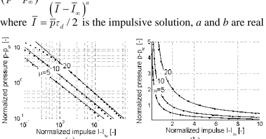
The general formulae proposed to fit the numerical results is written in a traditional interaction way
a b p p I I (31)where I pτd / 2 is the impulsive solution, a and b are real coefficients.
The two coefficients a and b are determined by using the least mean square, with a focus on the dynamic part of the iso-damage curves.
Fig. 5 (a) and (b) illustrate the iso-damage curves in both logarithmic and cartesian axes for ξ=2%, θy=13
mrad, ψM=20, ψK=1. The lines fit
well the iso-damage curves (Fig. 5 (a)) although there is an increasing error for extreme behaviour.
An extensive simulation study covering the practical ranges of the dimensionless parameters has resulted in these analytical expressions of the coefficients a and b:
3 2
1 2 3
6, 7.10 0, 7332 ;
a μ b B μ B μB (32)
where B1, B2 and B3 are coefficients depending on ψK, ξ and α (assumption that β=1 and γ=1).
This analytical procedure is valid for 5≤ μ≤ 20; 15≤ 2l/h≤ 30; 0.5≤ ψK≤ 2; 5≤ ψM≤ 20 and 0.4≤ τd ≤ 40.
If τd<0.4 or τd>40, the asymptotic solutions should be preferred since they give accurate results.
4.5 Accuracy of the dynamic regime solution
We proceed in the same way to assess the error of the solution (31) in the dynamic regime. First, the iso-damage curve corresponding to a level of protection is computed numerically. Then, this curve is read from the impulsive case (τd =0.4) to the Q.-S.
Fig. 5:Iso-damage curves for ξ=2%, θy=13 mrad, ψM=20,
ψK=1, α=2, β=1, γ=1 (a) in logarithmic and (b) cartesian
axes. Numerical result: •; Linear fitting of curves: — .
(a) (b)
limit (τd =40) in order to collect a series of blast loadings
p I, .Finally, for each couple
p I, , the demand of ductility is computed by using the analytical procedure (31).Fig. 6 illustrates the relative error on the ductility for variable parameters ψK (ψM=20), ξ and a parabolic M-N plastic interaction,
α=2, β=1, γ=1. Only the second level of protection is considered since the relative error increases with ductility. The relative error is higher at extreme behaviour, it peaks at 4 %. The coefficients a and b are fitted by considering that ψM is
equal to 20. If this parameter is decreased to 5, the relative error is still bounded to 5 %. Moreover, if an M-N linear plastic interaction is selected, α=1, β=1, γ=1, the relative error remains below 5 %.
5.
Conclusions
In this paper, we have derived analytical solutions for the response of a beam subjected blast loading taking into account the lateral restraint and inertia offered by the rest of the structure. The main goal was to propose a full analytical method depending on the six dimensionless parameters of this well-posed problem. We came up with an analytical formulation for the quasi-static assumption (τd>40), an iterative analytical procedure for the impulsive asymptote (τd<0.4), and an
analytical solution in the intermediate dynamic regime. In all cases, the relative error on ductility is shown not to exceed 6 % for realistic ranges of values of the dimensionless parameters.
Acknowledgment
The authors thank “Fonds de la Recherche Fondamentale Collective (FRFC)” for its financial support through the project N°6839853.
References
[1] MAYS G.C. and SMITH P.D., Blast effects on buildings: Design of buildings to optimize resistance to blast loading. Thomas Telford, pp. 59-61, 1995.
[2] LI Q.M. and MENG H., “Pulse loading shape effects on pressure – impulse diagram of an elastic – plastic single-degree-of-freedom structural model”, International journal of mechanical sciences, 44(9), pp. 1985–1998, 2002.
[3] LANGDON G.S. and SCHLEYER G.K., “Inelastic deformation and failure of profiled stainless steel blast wall panels. Part II: analytical modelling considerations”, Int. J. Impact Eng., vol. 31, no. 4, pp. 371–399, Apr. 2005.
[4] FALLAH A.S. and LOUCA L.A., “Pressure–impulse diagrams for elastic-plastic-hardening and softening single-degree-of-freedom models subjected to blast loading”, Int. J. Impact Eng., vol. 34, no. 4, pp. 823–842, Apr. 2007.
[5] HAMRA L., DEMONCEAU J.-F., DENOEL V., “Pressure-impulse of a beam under explosion – Influence of the indirectly affected part”, Proceedings of the 7th European Conference on Steel and Composite Structures, September 2014.
[6] VILETTE M., Critical analysis of the treatment of members subjected to compression and bending and propositions of new formulations (in French), Phd Thesis. Liege University, 2004.
[7] EUROPEAN COMMITTEE for standardization, “EN 1993-1-1. Eurocode 3: Design of steel structures - Part 1-1: General rules and rules for buildings,” 2005.
[8] US Army, “Structures to resist the effects of accidental explosions.” TM5-1300, pp. 1400, Fig. 6: Relative error on ductility obtained by the
approx-imate dynamic solution for the second category of protec-tion (a) ξ=1 %, θy=15 mrad and (b) ξ=2 %, θy=10 mrad
(c) ξ=2.8 %, θy=9 mrad. (ψM=20, ψK variable, α=2, β=1,
γ=1)