www.atmos-meas-tech.net/3/1457/2010/ doi:10.5194/amt-3-1457-2010
© Author(s) 2010. CC Attribution 3.0 License.
Measurement
Techniques
Validation of five years (2003–2007) of SCIAMACHY CO total
column measurements using ground-based spectrometer
observations
A. T. J. de Laat1,2, A. M. S. Gloudemans2,†, H. Schrijver2, I. Aben2, Y. Nagahama3, K. Suzuki4, E. Mahieu5, N. B. Jones6, C. Paton-Walsh6, N. M. Deutscher6, D. W. T. Griffith6, M. De Mazi`ere7, R. L. Mittermeier8, H. Fast8, J. Notholt9, M. Palm9, T. Hawat10, T. Blumenstock11, F. Hase11, M. Schneider11, C. Rinsland12, A. V. Dzhola13, E. I. Grechko13, A. M. Poberovskii14, M. V. Makarova14, J. Mellqvist15, A. Strandberg15, R. Sussmann16, T. Borsdorff16, and M. Rettinger16
1KNMI Royal Netherlands Meteorology Institute, de Bilt, The Netherlands 2SRON Netherlands Institute for Space Research, Utrecht, The Netherlands
3Graduate School of Environment and Information Sciences, Yokohama National University, Japan 4Yokohama University, Yokohama, Japan
5Institute of Astrophysics and Geophysics, University of Li`ege, Belgium 6School of Chemistry, University of Wollongong, Wollongong, NSW, Australia 7Belgian Institute for Space Aeronomy (BIRA-IASB), Brussels, Belgium 8Air Quality Research Division, Environment Canada, Toronto, ON, Canada 9Institute of Environmental Physics, University of Bremen, Germany
10Department of Physics and Astronomy, Denver University, Denver, CO, USA 11IMK-ASF, Karlsruhe Institute of Technology, Karlsruhe, Germany
12NASA Langley Research Center, Hampton, VA, USA
13Physial Faculty, St. Petersburg State University, St. Petersburg, Russia 14Institute of Atmospheric Physics, RAS, Moscow, Russia
15Radio and Space Science, Chalmers University of Technology, G¨oteborg, Sweden 16Karlsruhe Institute of Technology, IMK-IFU, Garmisch-Partenkirchen, Germany †sadly passed away 11 October 2010
Received: 16 April 2010 – Published in Atmos. Meas. Tech. Discuss.: 9 July 2010 Revised: 5 October 2010 – Accepted: 7 October 2010 – Published: 20 October 2010
Abstract. This paper presents a validation study of SCan-ning Imaging Absorption spectroMeter for Atmospheric CHartographY (SCIAMACHY) carbon monoxide (CO) to-tal column measurements from the Iterative Maximum Like-lihood Method (IMLM) algorithm using ground-based spec-trometer observations from twenty surface stations for the five year time period of 2003–2007.
Overall we find a good agreement between SCIAMACHY and ground-based observations for both mean values as well as seasonal variations.
Correspondence to: A. T. J. de Laat
For high-latitude Northern Hemisphere stations absolute differences between SCIAMACHY and ground-based mea-surements are close to or fall within the SCIAMACHY CO 2σ precision of 0.2 × 10¹⁸molecules/cm2 (∼10%) indicat-ing that SCIAMACHY can observe CO accurately at high Northern Hemisphere latitudes.
For Northern Hemisphere mid-latitude stations the valida-tion is complicated due to the vicinity of emission sources for almost all stations, leading to higher ground-based mea-surements compared to SCIAMACHY CO within its typical sampling area of 8◦×8◦.
Comparisons with Northern Hemisphere mountain sta-tions are hampered by elevation effects. After accounting for these effects, the validation provides satisfactory results.
At Southern Hemisphere mid- to high latitudes SCIA-MACHY is systematically lower than the ground-based mea-surements for 2003 and 2004, but for 2005 and later years the differences between SCIAMACHY and ground-based measurements fall within the SCIAMACHY precision. The 2003–2004 bias is consistent with previously reported results although its origin remains under investigation.
No other systematic spatial or temporal biases could be identified based on the validation presented in this paper.
Validation results are robust with regard to the choices of the instrument-noise error filter, sampling area, and time av-eraging required for the validation of SCIAMACHY CO total column measurements.
Finally, our results show that the spatial coverage of the ground-based measurements available for the validation of the 2003–2007 SCIAMACHY CO columns is sub-optimal for validation purposes, and that the recent and ongoing ex-pansion of the ground-based network by carefully selecting new locations may be very beneficial for SCIAMACHY CO and other satellite trace gas measurements validation efforts.
1 Introduction
The SCIAMACHY instrument (SCanning Imaging Absorp-tion spectroMeter for Atmospheric CHartographY; launched March 2002) onboard of the ENVISAT satellite (Bovens-mann et al., 1999) has provided over five years of carbon monoxide (CO) data based on reflected sunlight measure-ments in the short-wave infrared around 2.3 µm.
Validation of SCIAMACHY CO with Ground Based Spec-trometer (GBS) observations is complicated by the need for spatio-temporal averaging to obtain an acceptable precision of the SCIAMACHY CO columns. Furthermore, for most geolocations SCIAMACHY measures only once every six days. The irregular temporal sampling of the ground-based measurements and the occurrence of clouds significantly re-duces the number of truly collocated measurements. Com-bined with the sparse GBS network, validation of SCIA-MACHY CO observations with ground-based measurements has been quite limited so far.
Dils et al. (2006) presented a first validation using 11 GBS stations for one year (2003) of SCIAMACHY CO columns. Their results clearly showed that validation with GBS observations was difficult. They concluded that the data set used was too small to make an honest assess-ment of whether monthly mean values over their colloca-tion grid of 2.5◦×10◦ or 5◦×10◦ latitude-longitude do reach the target precision of 10% for CO. Furthermore, they found that the SCIAMACHY measurements for 2003 “exhibited clear flaws”.
Other validation studies used GBS observations at a single location on a mountain top (Sussmann and Buchwitz, 2005) or GBS measurements from a measurement campaign on board of a ship (Warneke et al., 2005).
Results from the Iterative Maximum Likelihood Method (IMLM) retrieval algorithm – developed at the Netherlands Institute for Space Research (SRON) – were also used in the Dils et al. (2006) study. However, this algorithm has been improved since and the length of the observational record now covers five years (2003–2007) including observations over both land and oceans (Gloudemans et al., 2009). The ocean observations greatly improve the spatial coverage of SCIAMACHY CO observations considerably and enhance the possibilities for validation of SCIAMACHY CO total col-umn measurements with GBS measurements as a number of GBS stations are located on islands or close to sea.
In this paper we present a validation of five years (2003–2007) of SCIAMACHY CO observations from the IMLM algorithm using twenty GBS stations. In previous studies we used the TM4 chemistry-transport model to quan-tify various effects that hamper the validation (de Laat et al., 2007, 2010; Gloudemans et al., 2009). This approach is also used in this study. SCIAMACHY measurements do not pro-vide any information about the vertical distribution of CO, making the GBS CO total column measurements the obvi-ous observational data for validation rather than aircraft data and vertical CO profiles used for the validation of infrared satellite measurements of CO.
This paper is organized as follows: Sect. 2 briefly de-scribes the IMLM retrieval algorithm, GBS measurements and the TM4 model. Section 3 shows the GBS observations and describes the choice of the sampling area. Section 4 presents the validation of the SCIAMACHY CO measure-ments using the GBS observations, and in Sect. 5 we inves-tigate the sensitivity of the validation results to the sampling area size, instrument-noise error filter, and the target preci-sion. Section 6 ends the paper with a summary and conclu-sions.
2 Datasets
2.1 SCIAMACHY CO
For this study we use SCIAMACHY CO total columns re-trieved with the IMLM algorithm version 7.4 in the short-wave infrared short-wavelength range between 2324.5–2337.9 nm (Gloudemans et al., 2008, 2009). This spectral region is sen-sitive to the whole column, with almost uniform sensitivity from 200 hPa down to the surface (Gloudemans et al., 2008). In this paper, we assume that the SCIAMACHY CO total column is the real total column. De Laat et al. (2010) esti-mated that the effects of the SCIAMACHY CO a priori and averaging kernel were of the order of only a few percent.
Single SCIAMACHY CO measurements have large instrument-noise errors – typically of the order of 10–100% of the total CO column value (de Laat et al., 2007). Hence, obtaining valuable information about CO from SCIA-MACHY requires averaging multiple measurements and
Fig. 1. Location of GBS stations listed in Table 1. The color coding of the stations is the same as in Fig. 2.
weighing them with their corresponding instrument-noise errors. Several studies have shown that reducing the instrument-noise error by averaging multiple measurements yields useful information about CO (de Laat et al., 2006, 2007, 2010; Gloudemans et al., 2006, 2009). De Laat et al. (2007) estimated the SCIAMACHY CO precision is ap-proximately 1 × 10¹⁷molecules/cm2.
In this study we use the averaging method introduced in Gloudemans et al. (2009) where observations for a selected area are averaged in time until a given threshold noise error is reached. The standard threshold instrument-noise error used in this paper is 1 × 10¹⁷molecules/cm2. We thus construct a time series of time-area average SCIA-MACHY observations for which the time intervals vary in length, but the averages all have the same instrument-noise error (rather than having averages for constant time intervals but with varying instrument-noise errors). This time series then is compared to the GBS observations. If multiple GBS observations fall within a SCIAMACHY CO time-interval, they are averaged arithmetically. We vary neither the area size nor the threshold instrument-noise error during the av-eraging procedure. However, we will test the sensitivity of our results to choices in area size and instrument-noise er-rors later on. Finally, we use SCIAMACHY CO observations over both land as well as ocean measurements over low alti-tude clouds between the surface and 800 hPa using the same selection criteria as in Gloudemans et al. (2009) and de Laat et al. (2010). This greatly improves spatio-temporal cover-age as discussed in these papers. However, using measure-ments over low altitude clouds means that only the partial CO column above the cloud is observed. The effect this has on the validation is quantified by estimating the below-cloud CO partial column from TM4 model results.
Table 1. Geographical information of the GBS stations used in this study. Stations are ordered from South to North according to their respective latitudes. Indicated in the second column are the databases where the measurements were obtained (N = NDACC; C = NILU CalVal; R = Research Institutes). Note that all stations, except Darwin, Garmisch-Partenkirchen, Zvenigorod and St. Pe-tersburg, are associated with NDACC.
Station Lat N Lon E Altitude (m) Available years Arrival Heights C −77.8 166.6 200 3/4/5/6/7 Lauder N −45.0 169.7 370 3/4/5/6/7 Wollongong N −34.5 150.9 30 3/4/5/6 R´eunion N −20.9 55.5 50 4/7 Darwin R −14.2 130.9 0 5/6/7 Mauna Loa N 19.5 −155.6 3397 3/4/7 Iza˜na N 28.3 −16.5 2367 3/4/5/6/7 Kitt Peak N 31.9 −111.2 2090 3/4/5 Rikubetsu R 43.5 −143.8 280 3/4/5/6/7 Egbert C 44.2 −79.8 280 3/4 Moshiri R 44.4 −142.3 370 3/4/5/6/7 Jungfraujoch R 46.5 8.0 3580 3/4/5/6/7 Zugspitze N 47.4 11.0 2964 3/4/5/6/7 Garmisch- R 47.4 11.1 734 4/5/6/7 Partenkirchen Bremen N 53.1 8.9 27 3/4/5/6/7 Zvenigorod C 55.7 36.8 200 4/5/6/7 St. Petersburg C 59.9 29.8 30 4/5/6/7 Harestua N 60.2 10.8 596 3/4/5/6/7 Kiruna N 67.8 20.4 419 3/4/5/6/7 Ny Alesund N 78.9 11.9 20 3/4/5/6/7 2.2 Ground-based data
The ground-based CO observations used in this study are col-lected at twenty locations worldwide, mainly from Fourier Transform Spectrometers (Fig. 1). The locations and alti-tudes of the stations are summarized in Table 1. The GBS ob-servations represent daytime solar absorption measurements under clear sky conditions. For most stations CO columns from thermal infrared spectra around 4.7 µm have been used, except for Darwin for which the short-wave infrared CO spectral features around 2.3 µm are used – the same spectral window as used for the SCIAMACHY CO retrievals. For the two Russian stations Zvenigorod and St-Petersburg CO total column amount are derived based on direct solar IR spectra in the 4.7 µm CO absorption band using grating spectrom-eters (spectral resolution ∼0.2–0.4 cm−1)equipped with a sun-tracking system (Dianov-Klokov, 1984; Dianov-Klokov et al., 1989; Mironenkov et al., 1996; Makarova et al., 2004). For ten of the stations data has been obtained from the public database from the Network for the Detection of Atmo-spheric Composition Change (NDACC; http://www.ndacc. org) (cf. Table 1). Additionally, measurements for five sta-tions were taken from the CalVal ENVISAT ground-based measurement and campaign database at the NADIR data centre of the Norwegian Institute for Atmosphere Research (NILU) (http://nadir.nilu.no/calval/). For the Jungfraujoch
station the measurement data used here were obtained di-rectly from the University of Li`ege. Data from the R´eunion station were provided by the Belgian Institute for Space Aeronomy (BIRA) (Senten et al., 2008; Duflot et al., 2010), and observations for Darwin have been kindly provided by the University of Wollongong (Paton-Walsh et al., 2010; Deutscher et al., 2010). Observations from Garmisch-Partenkirchen were provided by the Karlsruhe Institute of Technology (IMK-IFU) in Garmisch-Partenkirchen (Bors-dorff and Sussmann, 2009). Both Darwin and Garmisch-Partenkirchen are official TCONN sites (Total Carbon Col-umn Observing Network Toon et al., 2009). Measurements from two Japanese stations, Rikubetsu and Moshiri, were provided by the Solar-Terrestrial Environment Laboratory (STEL) of Nagoya University in Japan. A description of both Japanese sites and analysis of the measured CO columns for the period 1997–2005 can be found in Nagahama and Suzuki (2007).
Typical reported errors for GBS columns are 5% or less, although this varies from station to station. Nevertheless, these errors are considerably smaller than the single SCIA-MACHY CO column measurements and also smaller than the estimated SCIAMACHY precision, hence we ignore GBS errors for the remainder of the paper.
The effect of the GBS averaging kernels – also referred to as “smoothing error” – is small. Barret et al (2003) reports a smoothing error of 0.6% for the Jungfraujoch measurements while Senten et al. (2008) reports a smoothing error of 0.3% for La R´eunion. Both studies use infrared measurements. Paton-Walsh et al. (2005) reports a smoothing error of 5.8% for Darwin for near-infrared measurements around 2.3 µm, similar to the smoothing error reported for SCIAMACHY (de Laat et al., 2010) which also observes at the same wave-lengths.
2.3 Global chemistry-transport model TM4
We use the TM4 chemistry-transport model for the years 2003 to 2007 to quantify various effects that are important for the comparison of SCIAMACHY and GBS measurements. This model was also used in de Laat et al. (2007, 2010) and Gloudemans et al. (2009) and is described in more de-tail in Meirink et al. (2006). The horizontal resolution of TM4 is 3◦×2◦ longitude-latitude, and vertically 25 levels are used for years prior to 2006 and 34 levels from 2006 onwards because of a change in the number vertical lay-ers – from 60 to 91 – used by the European Centre for Medium-Range Weather Forecasts (ECMWF) for their op-erational data. Meteorological ECMWF analysis input fields used in TM4 are pre-processed as described in Bregman et al. (2003). Actual biomass burning emission estimates are taken from the Global Fire Emission Database (GFED), ver-sion 2 (van der Werf et al., 2006). Anthropogenic emisver-sions are based on the EDGAR v3 emission database (van Aar-denne et al., 2001) and are modified to be representative of
the year 2000 with a total of 331 Tg CO/year for fossil fuels (Dentener et al., 2003). Oceanic and natural emissions are 40 and 75 Tg CO/year, respectively, as described in Houwel-ing et al. (1998). Total biogenic emissions are 94 Tg CO/year (Dentener et al., 2003).
De Laat et al. (2007, 2009) presented validation of this model simulation for two years of observations using in situ surface CO measurements from the Global Monitoring Di-vision (GMD) database. The results showed that in the Southern Hemisphere (SH) average CO surface concentra-tions agree very well, whereas in the Northern Hemisphere (NH) the model underestimates surface CO by 10–20% for nearly all stations. The agreement was better for background stations than for stations close to large emission sources and the seasonal cycle of remote locations was closely matched by the model. These results suggest that the observed spatio-temporal CO variability is well reproduced by the model but that the model results contain a widespread Northern Hemisphere bias. This finding is consistent with Shindell et al. (2006) who drew similar conclusions based on a multi-model analysis of CO using both satellite and in situ mea-surements, and who attributed this bias to underestimated East Asian emissions in the TM4 model.
3 Comparisons with GBS measurements 3.1 GBS columns and seasonal cycles
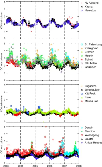
Figure 2 shows the variations of the GBS CO total columns available for the 2003–2007 time period. In the Northern Hemisphere (Fig. 2a–c) seasonal variations dominate CO variability for most stations, with a wintertime maximum and summertime minimum related to photochemical destruction by OH, which is strong during boreal summer and weak dur-ing boreal winter. This leads to accumulation of CO in the Northern Hemisphere during autumn and winter and a strong decrease of CO during spring. A detailed discussion of the CO seasonality as seen in GBS observations can be found in Yurganov et al. (2005).
The largest amplitudes occur for the Russian locations in Zvenigorod and St. Petersburg and the Japanese stations Moshiri and Rikubetsu (Fig. 2b). The Russian stations can be affected by nearby forest and peat fires and are close to isolated major industrial areas (Yurganov et al., 2008). The Japanese stations are located under the outflow of East Asian pollution (Koike et al., 2006) and can also be influenced by Siberian fires (Nagahama and Suzuki, 2007). The Bre-men, Garmisch-Partenkirchen and Egbert stations show sea-sonal cycles more similar to the Northern Hemisphere high-latitude stations in Fig. 2b where the variability is dominated by photochemical destruction of OH.
Figure 2c shows seasonal cycles of Northern Hemisphere mountain stations. The CO columns and amplitudes of the seasonal cycles are smaller than the Northern Hemisphere
Fig. 2. Time series of the twenty GBS stations measuring CO to-tal columns (1018molecules/cm2; individual measurements) for the period 2003–2007. Stations are ordered from North to South ac-cording to their latitude (Table 1).
high-latitude stations which is related to the missing lowest 2–3 km of the troposphere where large emissions and photo-chemical destruction occur. Note that for Kitt Peak no obser-vations are available beyond 2005 (Fig. 2c).
Figure 2d shows the Southern Hemisphere stations, where the seasonal cycle is shifted by 6 months compared to the Northern Hemisphere stations. Both Arrival Heights and Lauder are remote from CO sources and show little varia-tion on short timescales. On the other hand, Wollongong and Darwin, Australia, are located close to emission sources and show large increases in CO related to near-by forest fires (Paton-Walsh et al., 2005, 2009). For R´eunion limited ob-servations are available but nevertheless the increase in CO during the tropical biomass burning season in the southern half of Africa is present, when R´eunion is located under out-flow of African biomass burning plumes (Duflot et al., 2010; Senten et al., 2008).
3.2 The area for comparison
Because of the large SCIAMACHY CO instrument-noise er-rors a direct comparison of individual SCIAMACHY mea-surements with GBS CO total columns is not valuable. As a result, spatial and/or temporal averaging of the SCIA-MACHY CO columns is required to reduce the instrument-noise error. As explained in Sect. 2.1, we use spatio-temporal averaging where for a selected area around the ground-based station – the so-called sampling area, we av-erage in time until a threshold instrument-noise error of 1 × 10¹⁷molecules/cm2is reached. A weighted average is computed using the SCIAMACHY instrument-noise errors as the scaling factor (cf. de Laat et al., 2007).
Two considerations are important for deciding on an opti-mal sampling area. The larger the sampling area, the more SCIAMACHY CO measurements are available, and thus the smaller the temporal resolution of the average. However, the larger the sampling area, the less representative the corre-sponding SCIAMACHY CO column may be of the true lo-cal CO column derived from ground based GBS measure-ments. There thus is a trade-off between the sampling area size and the time resolution. We calculated three statis-tics of the SCIAMACHY-GBS comparison for sampling square area sizes ranging from 1◦×1◦ to 20◦×20◦ lati-tude and longilati-tude: the mean bias, root-mean-square (rms) difference – which is a measure for the representativeness of the selected area and the scatter in the measurements – and the total number of SCIAMACHY measurements used for the comparison.
Figure 3a shows the mean SCIAMACHY-GBS difference as a function of sampling area size for each GBS location and Fig. 3b shows that the root-mean-square of the differ-ences between SCIAMACHY and GBS CO total columns. The largest change in the absolute and rms difference oc-curs for small sampling area sizes. Beyond a sampling area size of 8◦×8◦ degrees differences remain nearly constant. This indicates that with increasing sampling area size the SCIAMACHY CO columns become less representative of the GBS locations. Figure 3c shows that the number of SCIAMACHY measurements used in the comparison in-creases with increasing sampling area size – as expected. For the best SCIAMACHY-GBS comparison one would like the rms differences to be as small as possible – i.e. a small sam-pling area (Fig. 3b) – yet the number of observations as large as possible – i.e. a large sampling area (Fig. 3c). Hence, the deciding factor is the change of the mean difference as func-tion of the sampling area (Fig. 3a). Since beyond a sampling area of 8◦×8◦ the mean differences do not change much, we start by investigating results for the smallest area size be-yond which the differences are more or less constant, which is a square area of 8◦×8◦degrees around the GBS location. However, because of the weak dependence of rms differences on sampling area size we will later on also discuss validation results for larger sampling area sizes.
Fig. 3. Average (A) and root-mean-square (B) differences between SCIAMACHY and GBS CO total columns as function of the sam-pling area size in which SCIAMACHY observations are used. Panel (C) shows the number of SCIAMACHY observations available for comparison for each area size. The area is defined as a square box with dimensions varying from 1◦×1◦to 20◦×20◦degrees.
Figure 4 shows a scatter plot of all GBS CO total columns and corresponding SCIAMACHY CO total columns for the 8◦×8◦degree areas, using the method described above. The scatter plot shows that the observations are close to the 1:1 line, but there is a considerable scatter and there are clear dif-ferences between locations. In the next section the difference for each station are discussed in detail.
Fig. 4. Scatter plot of SCIAMACHY and GBS CO total columns for all GBS stations for the period 2003–2007. The sampling area size is 8◦×8◦. The dashed lines denote the 1:1 line and the zero level. In case of SCIAMACHY observations over low-altitude ocean clouds no correction is added for the missing below-cloud partial columns.
4 Validation results
4.1 Southern Hemisphere locations
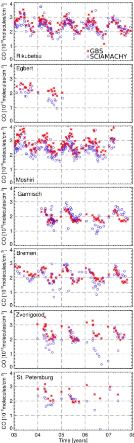
Figure 5a shows the time series of GBS and SCIAMACHY CO total columns for the Southern Hemisphere locations Ar-rival Heights, Lauder, Wollongong, Darwin, and R´eunion. The corresponding statistics can be found in Table 2. For these stations the 8◦×8◦sampling area includes many mea-surements over clouded ocean scenes. For these measure-ments the part of the column below the cloud is estimated based on TM4 model results and is added to the mea-sured SCIAMACHY column above the cloud (cf. Sect. 2.1; Gloudemans et al., 2009; de Laat et al., 2010). For Ar-rival Heights we only took SCIAMACHY observations over oceans because over land SCIAMACHY observes mainly over the high altitude interior of Antarctica causing an al-titude difference. The SCIAMACHY and GBS observa-tions show similar seasonal cycles, but SCIAMACHY un-derestimates the CO total columns on average by 0.1– 0.49 × 10¹⁸molecules/cm2 (Table 2). As noted in de Laat et al. (2010), south of 45◦S the SCIAMACHY CO to-tal columns are approximately 0.15 × 10¹⁸molecules/cm2 smaller than TM4 model results for the period 2004–2005, in line with the average differences between SCIAMACHY and GBS for Arrival Heights and Lauder (Table 2) for these two years. Note that for the remote Southern Hemisphere TM4 results showed hardly any bias compared to in situ sur-face observations (de Laat et al., 2007).
For R´eunion, despite limited data, both GBS and SCIA-MACHY measurements show a similar seasonal increase in CO related to the Southern Africa biomass-burning season. For Darwin, seasonal cycles agree although SCIAMACHY
Fig. 5a. Time series of the SCIAMACHY-GBS comparison for five Southern Hemisphere stations for the results presented in Fig. 4. For SCIAMACHY ocean measurements the estimated TM4 column below the cloud has been added to the SCIAMACHY CO partial column.
appears to slightly underestimate CO in 2006. Neverthe-less, Table 2 shows that the average differences for both R´eunion and Darwin are small and close to the estimated SCIAMACHY precision.
Differences for Wollongong are larger than for the other stations, but Wollongong is affected by local forest fires and orography that increase local CO amounts. As a result, Wol-longong GBS CO total columns are less representative of the surrounding areas as measured by SCIAMACHY than the Arrival Heights and Lauder CO total columns.
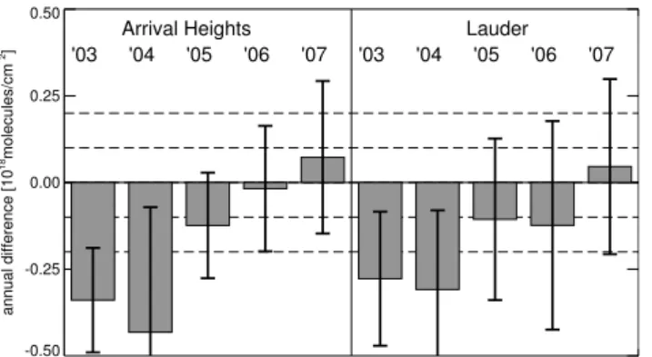
For year to year changes, the comparison at Arrival Heights and Lauder shows that the bias is not constant over time (Fig. 5e). Annual mean differences between SCIA-MACHY and GBS for 2003 and 2004 are −0.34 × 10¹⁸ and −0.43 × 10¹⁸molecules/cm2 for Arrival Heights and
−0.28 × 10¹⁸ and −0.31 ×1 018molecules/cm2 for Lauder, respectively. For 2005, 2006 and 2007 the differences are
−0.12 × 10¹⁸, −0.02 × 10¹⁸and 0.07 × 10¹⁸molecules/cm2 for Arrival Heights and −0.11 × 10¹⁸, −0.12 × 10¹⁸ and 0.05 × 10¹⁸ for Lauder, respectively. These differences are considerably smaller than the differences for the years 2003 and 2004 and are close to or within the estimated SCIAMACHY precision. A similar behavior is not found for other locations. The origin of the SCIAMACHY Southern Hemisphere middle and high latitude bias is currently under investigation.
The rms differences are larger than what is expected based on the instrument-noise error. This may to some extent be related to representation differences, i.e. SCIAMACHY av-erages are representative for a larger area than the GBS aver-ages. As a result, it can be expected that for larger compar-ison areas the rms differences increase, and that larger rms differences occur for GBS locations that are more affected by local emissions. Stations affected by local emissions like the European continental stations or the Australian stations Dar-win and Wollongong have larger rms differences than more remote high latitude European and Southern Hemisphere sta-tions like Lauder and Arrival Heights (Fig. 3b and Table 2). 4.2 Northern Hemisphere mountain stations
Figure 5b and Table 2 show the results for the high-altitude locations Iza˜na (Canary Islands), Mauna Loa, Jungfraujoch, Zugspitze and Kitt Peak. For Iza˜na and Mauna Loa we com-pare the GBS data with SCIAMACHY observations over cloudy ocean scenes with a cloud top height (CTH) corre-sponding to the altitude of the GBS stations. For Iza˜na we use clouds with a CTH between 800 and 700 hPa (2000– 3000 m), and for Mauna Loa we use clouds with a CTH be-tween 700 and 600 hPa (3000–4000 m).
For Iza˜na, Zugspitze, and Jungfraujoch seasonalities of SCIAMACHY and GBS are similar. The limited number of observations at Kitt Peak and Mauna Loa prohibits drawing conclusions about seasonal cycles.
For the mountain stations Jungfraujoch and Zugspitze SCIAMACHY columns are on average 0.76 × 10¹⁸ and 0.62 × 10¹⁸molecules/cm2 larger than GBS CO columns. However, the comparison for Garmisch-Partenkirchen (see also Table 2, Fig. 5c) – located at 745 m above sea level at the foot of the Zugspitze mountain – shows no signif-icant bias. The Jungfraujoch and Zugspitze measurement sites are located at approximately 3600 and 3000 m alti-tude, respectively. The SCIAMACHY measurements are more representative for the low altitude area north of the Alps as the average elevation within the 8◦×8◦ sampling
Fig. 5b. As Fig. 5a but for five Northern Hemisphere mountain stations. For Iza˜na and Mauna Loa SCIAMACHY CO columns with cloud top heights comparable to the station altitude were used (see text).
area around Zugspitze and Jungfraujoch which is only about 500 m which is comparable to the altitude of Garmisch-Partenkirchen. The mean difference in CO total columns between collocated Garmisch-Partenkirchen en Zugspitze measurements is 0.64 × 10¹⁸molecules/cm2, which is nearly similar to the SCIAMACHY-Zugspitze differences. The larger bias for Jungfraujoch compared to Zugspitze is related to the higher altitude of Jungfraujoch compared to Zugspitze: the CO columns for Jungfraujoch are clearly lower than those for Zugspitze (cf. Fig. 2c) whereas the SCIAMACHY measurements within the comparison areas round both sta-tions are comparable. Note that only taking SCIAMACHY
Fig. 5c. As Fig. 5a but for seven Northern Hemisphere mid-latitude stations.
observations over the Alps with ground scene altitudes simi-lar to that of Zugspitze or Jungfraujoch results is not possible due to insufficient SCIAMACHY collocations.
Kitt Peak (Arizona, USA) is located at 2100 m altitude sur-rounded by a high dry plateau remote from large CO sources. The SCIAMACHY 8◦×8◦ sampling area has an average altitude of 1000 m, but since the SCIAMACHY observa-tions are weighted with the instrument-noise error which is smaller for dry locations because of the higher surface re-flectance, and since dry locations have more cloud-free servations, the effective altitude of the SCIAMACHY ob-servations within the sampling area is about 1500 m, close to that of the Kitt Peak station. Hence, the mean SCIA-MACHY CO column should be representative for the Kitt Peak measurements. Indeed for Kitt Peak the differences be-tween SCIAMACHY and GBS (0.02 × 10¹⁸molecules/cm2; 1%) are well within the precision of the SCIAMACHY data. For Iza˜na differences also fall within the precision of the SCIAMACHY data: 0.09 × 10¹⁸molecules/cm2 (6%) because only SCIAMACHY observations over clouds with cloud top heights comparable to the Iza˜na station heights have been taken into account, and the location is remote of any large CO emission regions.
Mauna Loa shows a larger difference of 0.21 × 10¹⁸molecules/cm2 (20%) between SCIAMACHY and GBS, but this is still relatively small (twice the estimated SCIAMACHY precision). Given the limited number of correlative observations available for Mauna Loa (5) this larger difference may be a spurious result.
4.3 Northern Hemisphere mid-latitude low altitude stations
In this section we analyze observations from the low altitude stations Zvenigorod (near Moscow), St. Petersburg, Egbert (Canada), Garmisch-Partenkirchen and Bremen (Germany), Moshiri and Rikubetsu (Japan).
For Zvenigorod, St. Petersburg, and Egbert GBS columns are larger than SCIAMACHY columns by 0.53 × 10¹⁸, 0.44 × 10¹⁸ and 0.43 × 10¹⁸molecules/cm2, respectively (∼20%). All three stations are located close to large indus-trial areas or cities, which in case of the Russian locations are rather isolated CO sources. Furthermore, GBS measure-ments at Zvenigorod may also have been affected by local peat fires (Yurganov et al., 2009). The corresponding GBS measurements are thus likely affected by local emissions and therefore less representative for a larger SCIAMACHY sam-pling area around these locations. Note that for Zvenigorod the SCIAMACHY CO columns are unrealistically low in 2006. To a lesser extent this is also seen for St Petersburg and Bremen as well as for Jungfraujoch and Iza˜na. At the moment an explanation for this behavior is lacking.
The difference for Moshiri is −0.26 × 10¹⁸ molecules/cm2. However, approximately 150 km fur-ther south east at the location of Rikubetsu the difference
1
Figure 5D. As Figure 5A but for three Northern Hemisphere high latitude stations.
2
3
Figure 5E. Annual mean SCIAMACHY-GBS CO total column differences for the years
4
2003-2007 for Arrival Heights and Lauder in 10
18molecules/cm
2based on the results
5
presented in Fig. 5A. The dashed lines indicate the ± 1-σ or 2-σ SCIAMACHY precision
6
(0.1×10
18molecules/cm
2). The error bars indicate the 1-σ rms differences.
7
Fig. 5d. As Fig. 5a but for three Northern Hemisphere high latitude stations.
is only −0.10 × 10¹⁸molecules/cm2. Given the sampling area size of 8◦×8◦ there is considerable overlap in the SCIAMACHY measurements used for the comparisons for these stations, hence the variation in differences is unexpected. For both stations many ocean measurements are used in the comparison, but a check with clouds between the surface and 900 hPa rather than 800 hPa indicates that the differences between SCIAMACHY and GBS columns – including the filling of the SCIAMACHY columns with the TM4 values below the cloud – do not change significantly. Also, the differences hardly depend on the sampling area size (see Fig. 2), the bias difference is relatively small compared to the seasonal cycles, and there is an excellent agreement between SCIAMACHY and GBS seasonalities. This all suggests that the differences between Rikubetsu and Moshiri are robust. One possible explanation could be that Moshiri is slightly affected by local pollution, but this requires further investigation.
For Bremen and Garmisch-Partenkirchen differences are small at −0.11 × 10¹⁸ and 0.04 × 10¹⁸molecules/cm2, re-spectively, and very close to or smaller than the estimated SCIAMACHY precision. The seasonal cycles of SCIA-MACHY and GBS observations are comparable.
Fig. 5e. Annual mean SCIAMACHY-GBS CO total column dif-ferences for the years 2003–2007 for Arrival Heights and Lauder in 1018molecules/cm2 based on the results presented in Fig. 5a. The dashed lines indicate the ±1-σ or 2-σ SCIAMACHY precision (0.1 × 10¹⁸molecules/cm2). The error bars indicate the 1-σ rms differences.
4.4 Northern Hemisphere high latitude stations Harestua, Kiruna and Ny Alesund all show similar GBS-SCIAMACHY differences and seasonal cycles (Fig. 5d and Table 2). All three stations are located close to or within oceans, hence mostly ocean measurements are used in the comparisons. After addition of the partial CO col-umn below the cloud using TM4 results the differences be-come small compared to the 2-σ SCIAMACHY noise error:
−0.11 × 10¹⁸molecules/cm2for Harestua, −0.02 × 10¹⁸for Kiruna and −0.03 × 10¹⁸molecules/cm2 for Ny Alesund. For the latter two stations part of the seasonal cycle can-not be observed for these locations as there are little or no SCIAMACHY observations available during Northern Hemispheric winter because of the high solar zenith angles. Nevertheless, the results show that the large springtime de-crease in CO in the Northern Hemisphere due to photochem-ical destruction is well captured in the SCIAMACHY obser-vations. Note that the 8◦×8◦sampling area for Harestua has a considerable overlap with the 8◦×8◦sampling area of Bre-men, hence it is not surprising that the SCIAMACHY-GBS differences between both stations are comparable (Table 2). The sampling areas for both these stations include a signif-icant amount of clouded ocean measurements for which the modeled column below the cloud may be slightly underes-timated (de Laat et al., 2010). Kiruna and Ny Alesund are located further north and remote from large Northern Hemi-sphere emission regions. The reported Northern HemiHemi-sphere model biases are smaller at high Northern latitudes (Shindell et al, 2006). Thus, the model bias can explain why the differ-ences between SCIAMACHY and GBS are less negative for Kiruna and Ny Alesund compared to Harestua and Bremen.
Fig. 6. Average differences between SCIAMACHY and GBS CO column measurements over the 2003–2007 period for an 8◦×8◦ sampling area (Table 2). The dashed bars indicate the average dif-ferences around the mean, the error bars indicate the root-mean-square of the differences and the solid red bars indicate the dif-ferences after adding the estimated TM4 column below the cloud for SCIAMACHY ocean measurements (not applied for Northern Hemisphere mountain stations).
4.5 Global validation results
Figure 6 summarizes the results for all stations. It can be seen that in case of SCIAMACHY clouded ocean measure-ments a substantial part of the total column can be located be-low the cloud and that the difference between SCIAMACHY and GBS is significantly reduced when including an esti-mate of the column below the cloud based on TM4 results. The SCIAMACHY CO bias south of 45◦S reported by de
Laat et al. (2010) is significant in 2003 and 2004 but is close to or within the SCIAMACHY precision for later years (Fig. 5e). Stations with strong local influences on GBS mea-surements such as Wollongong, Egbert, Moshiri, Zvenig-orod, and St. Petersburg clearly show a significantly lower SCIAMACHY columns compared to the GBS measurements and thus are not representative for the sampling area used for validating the SCIAMACHY CO columns. The moun-tain stations Zugspitze and Jungfraujoch are surrounded by
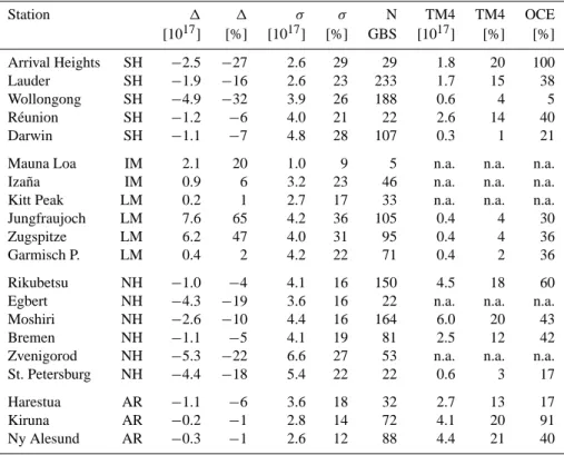
Table 2. Absolute (1) and root-mean-square (σ ) differences – in 1017molecules/cm2and percentage of the average measured total column – between SCIAMACHY and GBS 2003–2007 average CO total columns, the number of GBS observations used (N), the contribution of the TM4 filling below ocean cloud pixels (TM4) and the relative contribution of ocean pixels to the mean (OCE). The second column indicates the type of location: Southern Hemisphere (SH), island mountain (IM), land mountain (LM), Northern Hemisphere (NH and Arctic (AR). “n.a.” stands for “Not Available.” SCIAMACHY observations are sampled within 8◦×8◦degrees surrounding the GBS grid location and averaged, weighted by their respective noise errors. For the averaging one day at a time is added until the threshold instrument-noise error of 1 × 10¹⁷molecules/cm2is reached. If multiple GBS observations fall within the time range of the average SCIAMACHY CO total column then the GBS observations are averaged as well. If the sampling area includes clouded ocean measurements the results presented here include the SCIAMACHY below low-altitude cloud filling based on TM4 results, except for Iza˜na and Mauna Loa. As a result, for these locations no estimate is required for the missing ocean below-cloud partial column. In addition, Kitt Peak, Egbert and Zvenigorod are located too far away from oceans to have any ocean pixels contribute to the mean for an 8◦×8◦sampling area.
Station 1 1 σ σ N TM4 TM4 OCE [1017] [%] [1017] [%] GBS [1017] [%] [%] Arrival Heights SH −2.5 −27 2.6 29 29 1.8 20 100 Lauder SH −1.9 −16 2.6 23 233 1.7 15 38 Wollongong SH −4.9 −32 3.9 26 188 0.6 4 5 R´eunion SH −1.2 −6 4.0 21 22 2.6 14 40 Darwin SH −1.1 −7 4.8 28 107 0.3 1 21
Mauna Loa IM 2.1 20 1.0 9 5 n.a. n.a. n.a.
Iza˜na IM 0.9 6 3.2 23 46 n.a. n.a. n.a.
Kitt Peak LM 0.2 1 2.7 17 33 n.a. n.a. n.a.
Jungfraujoch LM 7.6 65 4.2 36 105 0.4 4 30
Zugspitze LM 6.2 47 4.0 31 95 0.4 4 36
Garmisch P. LM 0.4 2 4.2 22 71 0.4 2 36
Rikubetsu NH −1.0 −4 4.1 16 150 4.5 18 60
Egbert NH −4.3 −19 3.6 16 22 n.a. n.a. n.a.
Moshiri NH −2.6 −10 4.4 16 164 6.0 20 43
Bremen NH −1.1 −5 4.1 19 81 2.5 12 42
Zvenigorod NH −5.3 −22 6.6 27 53 n.a. n.a. n.a.
St. Petersburg NH −4.4 −18 5.4 22 22 0.6 3 17
Harestua AR −1.1 −6 3.6 18 32 2.7 13 17
Kiruna AR −0.2 −1 2.8 14 72 4.1 20 91
Ny Alesund AR −0.3 −1 2.6 12 88 4.4 21 40
low lying land regions, hence the SCIAMACHY and GBS measurements sample significantly different columns and thus these stations are not very appropriate for validating SCIAMACHY CO columns, as long as a robust correction method is not available to reproduce the low tropospheric CO columns in the Alpine region. The remaining stations show differences close to or within the estimated measure-ment precision of SCIAMACHY CO. The standard deviation of the differences as shown by the error bars in Fig. 6 is quite large for most stations and in particular for the stations with local influences. These standard deviations are larger than the typical GBS precision of <5%. The larger standard devi-ations are likely related to representation differences, which will be discussed in more detail in the following paragraph.
Finally, Table 2 shows that the model contribution to the SCIAMACHY total columns due to the filling of SCIA-MACHY ocean pixels for the FTIR locations can be as large
as 20%. This contribution depends on the missing below cloud partial column as well as the weighted averaging and the number of ocean pixels used for calculating the mean. On a global scale the below-cloud partial column are 16 ± 8% (2σ ) (de Laat et al., 2010; their Fig. 5a).
5 Sampling area, instrument-noise error and precision The SCIAMACHY columns used in the comparisons so far are based on spatio-temporal averaging of single mea-surements until a precision of 0.1 × 10¹⁸molecules/cm2 is reached. Single SCIAMACHY measurements with instrument-noise errors larger than 1.5 × 10¹⁸molecules/cm2 are excluded because of a clear retrieval bias for measure-ments with large instrument noise errors (de Laat et al., 2007). However, more stringent thresholds have not been tested. Also, the current IMLM retrieval version 7.4 includes
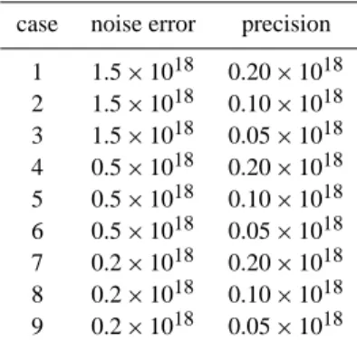
Table 3. SCIAMACHY parameter settings for cases presented in Fig. 7. Values are in molecules/cm2.
case noise error precision 1 1.5 × 10¹⁸ 0.20 × 10¹⁸ 2 1.5 × 10¹⁸ 0.10 × 10¹⁸ 3 1.5 × 10¹⁸ 0.05 × 10¹⁸ 4 0.5 × 10¹⁸ 0.20 × 10¹⁸ 5 0.5 × 10¹⁸ 0.10 × 10¹⁸ 6 0.5 × 10¹⁸ 0.05 × 10¹⁸ 7 0.2 × 10¹⁸ 0.20 × 10¹⁸ 8 0.2 × 10¹⁸ 0.10 × 10¹⁸ 9 0.2 × 10¹⁸ 0.05 × 10¹⁸
a more realistic calculation of the instrument-noise error (Gloudemans et al., 2009). The precision threshold of 0.1 × 10¹⁸molecules/cm2 used in this paper corresponds to the upper limit of the 0.05–0.1 × 10¹⁸molecules/cm2 range of the monthly mean precision derived by de Laat et al. (2007). The SCIAMACHY CO precision de facto thus could be smaller.
In this section we briefly discuss the effect of filtering single SCIAMACHY measurements on different instrument-noise errors and the effect of using different precision thresholds in the spatio-temporal averaging on the valida-tion. Three SCIAMACHY instrument-noise error thresh-olds (1.5 × 10¹⁸, 0.5 × 10¹⁸, and 0.2 × 10¹⁸molecules/cm2)
and three SCIAMACHY precision thresholds (0.2 × 10¹⁸, 0.1 × 10¹⁸, and 0.05 × 10¹⁸molecules/cm2)are investigated, which results in nine different parameter combinations (Ta-ble 3). For each parameter set we calculate a skill score for the SCIAMACHY and GBS comparison for sampling areas ranging from 1◦×1◦to 20◦×20◦. The skill score is defined as (Taylor, 2001):
S = (1 + R)
2
(σf+1/σf)2
With S the skill level (varying between 0 and 1), R is the correlation coefficient and σf the ratio of the standard
devia-tions of two datasets. In cases where the standard deviadevia-tions of both data sets are comparable and the correlations are high (R close to 1) the skill level will be close to 1 and the two CO datasets are very similar. A skill level 0 indicates no resem-blance between the two data sets. Note that the skill level is not sensitive to systematic biases.
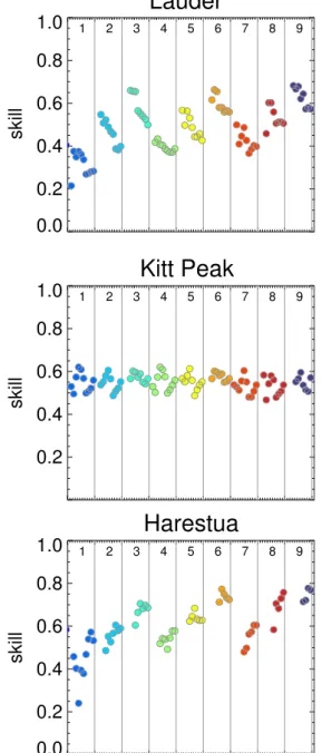
Figure 7 shows the skill value for three stations for all these combinations, which are numbered according to the combinations listed in Table 3. Similar plots for all stations can be found in the supplementary information. For each test, increasing sampling area sizes are represented going from small sizes on the left to large sizes on the right. Note that
experiment No. 2 represents the parameters values for the re-sults discussed in Sect. 4.
These three stations show very different behavior. For Lauder skill levels decrease with increasing sampling area size, but skill levels increase with a stricter instrument-noise error filter and for smaller precision thresholds. For Kitt Peak there is no change in skill for any of the three parameters. For Harestua, skill levels increase with increasing sampling area size, a stricter instrument-noise error filter and smaller precision thresholds.
In general, we found that for a stricter instrument-noise error threshold the skill levels remain similar for most sta-tions, although for some stations a slight increase is found (compare variations among parameter sets 1-4-7, 2-5-8 and 3-6-9). This increase appears to be restricted to stations with some SCIAMACHY outliers (see Fig. 5), which occur over European stations Zvenigorod, St. Petersburg, Bremen, and Jungfraujoch, Zugspitze and Garmisch-Partenkirchen.
Smaller precision thresholds increase the skill levels for most stations (compare variations among parameter sets 1-2-3, 4-5-6 and 7-8-9). This is related to the reduction of short-term variability in the CO column measurements when averaging more measurements over a longer period resulting in smaller precision thresholds. Short term varia-tions in CO columns are related to weather variability and air masses with different CO characteristics. They manifest themselves as random variations on top of the seasonal cy-cle. These random variations will differ between the SCIA-MACHY measurements averaged over the sampling area and GBS measurements, which as a result reduces the skill when comparing both. For longer time averages – required to re-duce instrument-noise errors – these random variations av-erage out. As a result, both the mean of SCIAMACHY and GBS CO columns become more representative of the actual long term mean and the seasonal cycle of CO, and as a consequence skill levels improve when using a stricter precision threshold.
For a number of GBS locations the comparison also improves by changing the sampling area size. However, the optimal choice for the sampling area size remains station dependent.
An example of the SCIAMACHY – GBS comparison as shown in Fig. 5 but for a different parameter set (number 6 in Table 2 for a 20◦×20◦ degree area) can be found in supplementary Fig. 2.
These results do not imply that a stricter instrument-noise error filter and smaller precision threshold should be used. Rather, it indicates that the signal-to-noise ratio of individual SCIAMACHY measurements is insufficient to derive use-ful information on short synoptic timescales. However, the results show that on monthly timescales or longer SCIA-MACHY observations do contain useful information.
Fig. 7. Skill score of the SCIAMACHY-GBS comparison for three stations Lauder, Kitt Peak and Harestua) for nine different parame-ter combinations as defined in Table 3, also indicated by the colors. The skill score, on a scale from zero to one, is a measure of the agreement between two series and is based on comparing the corre-lation between the two series and the root-mean-square error of the difference series (see text). The higher the skill score, the better the agreement. For each combination the skill scores are ordered from left to right from the smallest to the largest sampling area size. In addition, we excluded skill scores when less than 25 SCIAMACHY-GBS comparison values could be calculated.
6 Summary and conclusions
This paper presents a detailed validation of SCIAMACHY CO total columns with independent ground based CO total column observations from twenty GBS stations worldwide for the five-year period 2003–2007.
For all stations the seasonal cycle of SCIAMACHY and GBS agree well. For stations not affected by local emis-sions or altitude effects, differences between SCIAMACHY and GBS are close to or within the SCIAMACHY CO to-tal column precision of 0.1 × 10¹⁸molecules/cm2(∼5–10%) of the SCIAMACHY CO columns. Stations with strong local influences, such as Wollongong, Egbert, Zvenigorod, and St. Petersburg show significantly lower SCIAMACHY columns compared to the GBS stations. Because of the large SCIAMACHY sampling area of 8◦×8◦, local CO
enhance-ments as seen in the GBS measureenhance-ments do not show up in the SCIAMACHY average. Note that also the Moshiri sta-tion may be affected by some local influences.
For the Northern Hemisphere mountain locations Jungfraujoch and Zugspitze SCIAMACHY columns are significantly larger than those of the GBS stations. This can be explained by the specific geographical location of both stations. Mauna Loa also shows a bias but this may be a spurious result as there are relatively few measurements at this location.
The Southern Hemisphere stations Arrival Heights and Lauder show a clear bias for the years 2003 and 2004, which is not present for later years. The bias found is consistent with the Southern Hemisphere bias south of 45◦S mentioned in de Laat et al. (2010) and its origin is under investiga-tion. No other time dependent biases were identified, indi-cating that for now degradation of the SCIAMACHY CO channel seems to have only a minor effect on the retrieved columns – if any.
For most GBS locations a better agreement between SCIAMACHY and GBS is found when a stricter precision threshold is used, which is a consequence of the spatio-temporal averaging: when averaging CO column measure-ments over longer time periods the effect of short-time – often local – variability is reduced and the SCIAMACHY and GBS CO columns become more representative of the long-term CO column variability within the sampling area, and as a consequence the skill improves. This indicates that – because of the large instrument-noise error of single SCIAMACHY measurements – there is little information on timescales shorter than a month. However, it also shows that SCIAMACHY observations can be used to study seasonal and interannual CO total column variability.
Using a stricter instrument-noise error filter results in fewer outliers in the SCIAMACHY CO columns for some stations, suggesting that SCIAMACHY observations with larger instrument-noise errors may lead to anomalously small CO total columns.
Finally, although the validation of SCIAMACHY with GBS observations yields satisfactory results, there are clear limitations to this validation. The spatial coverage of GBS lo-cations is limited so that many important regions of the world are still missing, and SCIAMACHY measurements must be averaged over larger areas to lower the measurement noise. As a result, biases related to certain spatio-temporal surface parameters cannot be detected using the current set of avail-able GBS measurements. The recent and ongoing strong de-ployment of new GBS instruments as part of TCCON Dar-win and Garmisch as examples – will fill many gaps in the current GBS network.
Supplementary material related to this article is available online at:
http://www.atmos-meas-tech.net/3/1457/2010/ amt-3-1457-2010-supplement.pdf.
Acknowledgements. SCIAMACHY is a joint project of the German Space Agency DLR and the Dutch Space Agency NSO with con-tribution of the Belgian Space Agency. We thank the Netherlands SCIAMACHY Data Center and ESA for providing data. The work performed is (partly) financed by NSO. The authors also thank J. F. Meirink for providing the TM4 model data, the Network for the Detection of Atmospheric Composition Change (NDACC) for maintaining the GBS database and the various research groups for making their GBS observations available to the NDACC. The Solar-Terrestrial Environment Laboratory (STEL) of Nagoya University, Japan, is thanked for installing and operating the GBS stations at Moshiri and Rikubetsu and for providing the spectral data. The Darwin solar measurements and TCCON are funded by NASA’s terrestrial carbon cycle program, grant NNX08AI86G. Measurements at Bremen and Ny Alesund are partly financed by the EU-project HYMN and the DFG-project MESOSUB. We acknowledge the EU FP6 project GEOmon (project number 036677) for their support of the Zugspitze measurements.
Edited by: B. Funke
References
van Aardenne, J. A., Dentener, F. J., Olivier, J. G. J., Klein Gold-ewijk, C. G. M., and Lelieveld, J.: A 1◦×1◦ resolution data set of historical anthropogenic trace gas emissions for the period 1890 – 1990, Global Biogeochem. Cy., 15(4), 909–928, 2001. Barret, B., De Mazi`ere, M., and Mahieu, E.: Ground-based FTIR
measurements of CO from the Jungfraujoch: characterisation and comparison with in situ surface and MOPITT data, At-mos. Chem. Phys., 3, 2217–2223, doi:10.5194/acp-3-2217-2003, 2003.
Bovensmann, H., Burrows, J. P., Buchwitz, M., Frerick, J., Noel, S., Rozanov, V. V., Chance, K. V., and Goede, A. H. P.: SCIA-MACHY – Mission Objectives and Measurement Modes, J. At-mos. Sci., 56, 127–150, 1999.
Borsdorff, T. and R. Sussmann: On seasonality of stratomeso-spheric CO above midlatitudes: new insight from solar FTIR
spectrometry at Zugspitze and Garmisch, Geophys. Res. Lett., 36, L21804, doi:10.1029/2009GL040056, 2009.
Bregman, B., Segers, A., Krol, M., Meijer, E., and van Velthoven, P.: On the use of mass-conserving wind fields in chemistry-transport models, Atmos. Chem. Phys., 3, 447–457, doi:10.5194/acp-3-447-2003, 2003.
Buchwitz, M., de Beek, R., Bramstedt, K., No¨el, S., Bovensmann, H., and Burrows, J. P.: Global carbon monoxide as retrieved from SCIAMACHY by WFM-DOAS, Atmos. Chem. Phys., 4, 1945– 1960, doi:10.5194/acp-4-1945-2004, 2004.
Dentener, F., van Weele, M., Krol, M., Houweling, S., and van Velthoven, P.: Trends and inter-annual variability of methane emissions derived from 1979–1993 global CTM simulations, At-mos. Chem. Phys., 3, 73–88, doi:10.5194/acp-3-73-2003, 2003. Deutscher, N. M., Griffith, D. W. T., Bryant, G. W., Wennberg, P.
O., Toon, G. C., Washenfelder, R. A., Keppel-Aleks, G., Wunch, D., Yavin, Y., Allen, N. T., Blavier, J.-F., Jim´enez, R., Daube, B. C., Bright, A. V., Matross, D. M., Wofsy, S. C., and Park, S.: Total column CO2measurements at Darwin, Australia – site de-scription and calibration against in situ aircraft profiles, Atmos. Meas. Tech., 3, 947–958, doi:10.5194/amt-3-947-2010, 2010. Dianov-Klokov, V. I.: Spectroscopic studies of atmospheric
pol-lution over large cities, Izvestia AN SSSR, Fizika atmosfery i okeana, 20, 883–900, 1984 (in Russian).
Dianov-Klokov, V. I., Yurganov, L. N., Grechko, E. I., and Dzhola, A. V.: Spectroscopic measurements of atmospheric carbon monoxide and methane 1: Latitudinal distribution, J. Atmos. Chem., 8, 139–151, 1989.
Dils, B., De Mazi`ere, M., M¨uller, J. F., Blumenstock, T., Buchwitz, M., de Beek, R., Demoulin, P., Duchatelet, P., Fast, H., Franken-berg, C., Gloudemans, A., Griffith, D., Jones, N., Kerzenmacher, T., Kramer, I., Mahieu, E., Mellqvist, J., Mittermeier, R. L., Notholt, J., Rinsland, C. P., Schrijver, H., Smale, D., Strandberg, A., Straume, A. G., Stremme, W., Strong, K., Sussmann, R., Tay-lor, J., van den Broek, M., Velazco, V., Wagner, T., Warneke, T., Wiacek, A., and Wood, S.: Comparisons between SCIAMACHY and ground-based FTIR data for total columns of CO, CH4, CO2 and N2O, Atmos. Chem. Phys., 6, 1953–1976, doi:10.5194/acp-6-1953-2006, 2006.
Duflot, V., Baray, J. L., Dils, B., De Mazi`ere, M., Atti´e, J. L., Van-haelewyn, G., Senten, C., Vigouroux, C., Clain, G., and Del-mas, R.: Analysis of the origin of the distribution of CO in the subtropical southern Indian Ocean, J. Geophys. Res., in press, doi:10.1029/2010JD013994, 2010.
Gloudemans, A. M. S., Krol, M. C., Meirink, J. F., de Laat, A. T. J., van der Werf, G. R., Schrijver, H., van den Broek, M. M. P., and Aben, I.: Evidence for long-range transport of carbon monoxide in the Southern Hemisphere from SCIAMACHY observations, Geophys. Res. Lett., 33, L16807, doi:10.1029/2006GL026804, 2006.
Gloudemans, A. M. S., Schrijver, H., Hasekamp, O. P., and Aben, I.: Error analysis for CO and CH4total column retrievals from SCIAMACHY 2.3 µm spectra, Atmos. Chem. Phys., 8, 3999– 4017, doi:10.5194/acp-8-3999-2008, 2008.
Gloudemans, A. M. S., de Laat, A. T. J., Schrijver, H., Aben, I., Meirink, J. F., and van der Werf, G. R.: SCIAMACHY CO over land and oceans: 2003–2007 interannual variability, Atmos. Chem. Phys., 9, 3799—3813, doi:10.5194/acp-9-3799-2009, 2009.
Houweling, S., Dentener, F., and Lelieveld, J.: The impact of non-methane hydrocarbon compounds on tropospheric photochem-istry, J. Geophys., Res., 103, 10673–10696, 1998.
Koike, M., Jones, N. B., Palmer, P. I., Matsui, H., Zhao, Y., Kondo, Y., Matsumi, Y., and Tanimoto, H.: Seasonal variation of carbon monoxide in northern Japan: fourier transform IR measurements and source-labeled model calculations, J. Geophys. Res., 111, D15306, doi:10.1029/2005JD006643, 2006.
de Laat, A. T. J., Gloudemans, A. M. S., Schrijver, H., van den Broek, M. M. P., Meirink, J. F., Aben, I., and Krol, M.: Quantitative analysis of SCIAMACHY carbon monoxide to-tal column measurements, Geophys. Res. Lett., 33, L07807, doi:10.1029/2005GL025530, 2006.
de Laat, A. T. J., Gloudemans, A. M. S., Aben, I., Krol, M., van der Werf, G., Meirink, J. F., and Schrijver, H.: SCIA-MACHY Carbon Monoxide total columns: Statistical evalua-tion and comparison with CTM results, J. Geophys. Res., 112, D12310, doi:10.1029/2006JD008256, 2007.
de Laat, A. T. J., Gloudemans, A. M. S., Aben, I., and Schrijver, H.: Global evaluation of SCIAMACHY and MOPITT carbon monoxide column differences for 2004–2005, J. Geophys. Res., 115, doi:10.1029/2009JD012698, 2010.
Makarova, M. V., Poberovskii, A. V., and Timofeev, Y. M.: Tem-poral Variability of Total Atmospheric Carbon Monoxide over St. Petersburg. Izvestiya, Atm. Ocean Phys., 40, 3, 313–322, 2004.
Meirink, J. F., Eskes, H. J., and Goede, A. P. H.: Sensitivity analysis of methane emissions derived from SCIAMACHY observations through inverse modelling, Atmos. Chem. Phys., 6, 1275–1292, doi:10.5194/acp-6-1275-2006, 2006.
Mironenkov, A. V., Poberovskii, A. V., and Timofeev, Y. M.: In-terpretation of Infrared Solar Spectra for Quantification of the Column Content of Atmospheric Gases. Izvestiya, Atm. Ocean Phys., 32(2), 191–198, 1996.
Nagahama, Y. and Suzuki, K.: The influence of forest fires on CO, HCN, C2H6 and C2H2 over Northern Japan measured by in-frared solar spectroscopy, Atmos. Env., 41, 9570–9579, 2007. Paton-Walsh, C., Jones, N. B., Wilson, S. R., Haverd, V., Meier, A.,
Griffith, D. W. T., and Rinsland, C. P.: Measurements of trace gas emissions from Australian forest fires and correlations with coincident measurements of aerosol optical depth, J. Geophys. Res., 110, doi:10.1029/2005JD006202, 2005.
Paton-Walsh, C., Deutscher, N. M., Griffith, D. W. T., Forgan, B. W., Wilson, S. R., Jones, N. B., and Edwards, D. P.: Trace gas emissions from Savanna Fires in Northern Australia, J. Geophys. Res., 115, doi:10.1029/2009JD013309, 2010.
Senten, C., De Mazi`ere, M., Dils, B., Hermans, C., Kruglanski, M., Neefs, E., Scolas, F., Vandaele, A. C., Vanhaelewyn, G., Vigouroux, C., Carleer, M., Coheur, P. F., Fally, S., Barret, B., Baray, J. L., Delmas, R., Leveau, J., Metzger, J. M., Mahieu, E., Boone, C., Walker, K. A., Bernath, P. F., and Strong, K.: Technical Note: New ground-based FTIR measurements at Ile de La Runion: observations, error analysis, and comparisons with independent data, Atmos. Chem. Phys., 8, 3483–3508, doi:10.5194/acp-8-3483-2008, 2008.
Shindell, D. T., Faluvegi, G., Stevenson, D. S., Krol, M. C., Emmons, L. K., Lamarque, J.-F., P´etron, G., Dentener, F. J., Ellingsen, K., Schultz, M. G., Wild, O., Amann, M., Atherton, C. S., Bergmann, D. J., Bey, I., Butler, T., Cofala, J., Collins, W. J., Derwent, R. G., Doherty, R. M., Drevet, J., Eskes, H. J., Fiore, A. M., Gauss, M., Hauglustaine, D. A., Horowitz, L. W., Isaksen, I. S. A., Lawrence, M. G., Montanaro, V., M¨uller, J.-F., Pitari, G., Prather, M. J., Pyle, J. A., Rast, S., Rodriguez, J. M., Sanderson, M. G., Savage, N. H., Strahan, S. E., Sudo, K., Szopa, S., Unger, N., van Noije, T. P. C., and Zeng, G.: Multimodel sim-ulations of carbon monoxide: comparison with observations and projected near-future changes, J. Geophys. Res., 111, D19306, doi:10.1029/2006JD007100, 2006.
Sussmann, R. and Buchwitz, M.: Initial validation of EN-VISAT/SCIAMACHY columnar CO by FTIR profile retrievals at the Ground-Truthing Station Zugspitze, Atmos. Chem. Phys., 5, 1497–1503, doi:10.5194/acp-5-1497-2005, 2005.
Taylor, K. E.: Summarizing multiple aspects of model performance in single diagram, J. Geophys. Res., 106, D7, 7183–7192, 2001. Toon, G. C., Blavier, J. F., Washenfelder, R. A., Wunch, D., Keppel-Aleks, G., Wennberg, P. O., Connor, B. J., Sherlock, V., Griffith, D. W. T., Deutscher, N. M., and Notholt, J.: The Total Carbon Column Observing Network (TCCON), paper presented at Pro-ceedings of the Optical Society of America Fourier Transform Spectroscopy Meeting, Vancouver, April 2009.
Warneke, T., de Beek, R., Buchwitz, M., Notholt, J., Schulz, A., Ve-lazco, V., and Schrems, O.: Shipborne solar absorption measure-ments of CO2, CH4, N2O and CO and comparison with SCIA-MACHY WFM-DOAS retrievals, Atmos. Chem. Phys., 5, 2029– 2034, doi:10.5194/acp-5-2029-2005, 2005.
van der Werf, G. R., Randerson, J. T., Giglio, L., Collatz, G. J., Kasibhatla, P. S., and Arellano Jr., A. F.: Interannual variabil-ity in global biomass burning emissions from 1997 to 2004, At-mos. Chem. Phys., 6, 3423–3441, doi:10.5194/acp-6-3423-2006, 2006.
Yurganov, L. N., Duchatelet, P., Dzhola, A. V., Edwards, D. P., Hase, F., Kramer, I., Mahieu, E., Mellqvist, J., Notholt, J., Nov-elli, P. C., Rockmann, A., Scheel, H. E., Schneider, M., Schulz, A., Strandberg, A., Sussmann, R., Tanimoto, H., Velazco, V., Drummond, J. R., and Gille, J. C.: Increased Northern Hemi-spheric carbon monoxide burden in the troposphere in 2002 and 2003 detected from the ground and from space, Atmos. Chem. Phys., 5, 563–573, doi:10.5194/acp-5-563-2005, 2005.
Yurganov, L., McMillan, W. W., Dzhola, A. V., Grechko, E. I., Jones, N. B., and van der Werf, G.: Global AIRS and MO-PITT CO measurements: Validation comparison, and links to biomass burning variations and carbon cycle, J. Geophys. Res., 113, doi:10.1029/2007JD009229, 2008.
Yurganov, L., McMillan, W., Grechko, E., and Dzhola, A.: Anal-ysis of global and regional CO burdens measured from space between 2000 and 2009 and validated by ground-based solar tracking spectrometers, Atmos. Chem. Phys., 10, 3479–3494, doi:10.5194/acp-10-3479-2010, 2010.