Computing the cheapest winning coalition in a multi-agent game

(1)

HAL Id: dumas-00530790

https://dumas.ccsd.cnrs.fr/dumas-00530790

Submitted on 29 Oct 2010

HAL is a multi-disciplinary open access

archive for the deposit and dissemination of sci-entific research documents, whether they are pub-lished or not. The documents may come from teaching and research institutions in France or abroad, or from public or private research centers.

L’archive ouverte pluridisciplinaire HAL, est destinée au dépôt et à la diffusion de documents scientifiques de niveau recherche, publiés ou non, émanant des établissements d’enseignement et de recherche français ou étrangers, des laboratoires publics ou privés.

Computing the cheapest winning coalition in a

multi-agent game

Loïs Vanhée

To cite this version:

Loïs Vanhée. Computing the cheapest winning coalition in a multi-agent game. Computer Science and Game Theory [cs.GT]. 2010. �dumas-00530790�

(2)

Computing the cheapest winning coalition in

a multi-agent game

Lo¨ıs Vanh ´

ee

Supervisors:

Sophie Pinchinat

Scott Sanner

Sylvie Thiebaux

2010

Université de Rennes 1, Research unit: IRISA, Team: S4 Australian National University, Research unit: NICTA, Team: SMLG

IFSIC Research Master’s degree in Computer Science ENS Cachan, antenne de Bretagne

(3)

1 Introduction

To run a company, employers need to hire people to realize a product, a sport coach can motivate some players intend to win a match, a designer have to force synchronization of some parallel processes to avoid deadlocking. In these examples, a device external to the global system tries to force the behavior of some agents, aiming at achieving a global objective. For realism purposes, we assume that forming a coalition has a cost that should be minimal. This cost models the fact that individuals of the coalition may be deviated from their original objective. Game theory is a vast ﬁeld that addresses this kind of problem.

Depending on the type of games that are considered, the problem is more or less difficult to solve, and can be even non-computable. The inability for the agents to com-municate can lead to stupid solutions, where e.g. agents with compatible objectives may reach a deadlock. Therefore, some frameworks allow agents to communicate in order to team up: this is the “coalition formation” [21]. Agents of the coalition share a common strategy that fulfills every individual objective (otherwise a rational agent would not have joined it). The traditional coalition formation problem leads to extended problems of game theory: it focuses on issues such as determining whether some agents are always in a same coalition or not, whether negotiations terminate or not, etc. These kinds of is-sues tightly depend on the social welfare resolution and the payoff assignation mechanism [12]. In such theory, every agent cares only about her objective, without caring about the global objective. As we cannot know how non-hired agents can react, in particular their objectives may be in conflict with ours, these “opponents” may team up to prevent the outcome from being in our favor. In this case, the setting easily reduces to determine the winner in a 2-player game, namely the coalition against all other players.

In this work we focus on turn-based games, a simple and broadly explored branch of game theory. Turn-based games oﬀer well-known tools, among which the most famous minmax algorithm where a constrained optimization problem is addressed [19]. The problem we aim at solving is to ﬁnd a minimal cost coalition which enforces some position in a given set (the goal) to be eventually reached.

Note that the problem we handle can be represented by a derived game. Let us add a new agent am for “agent manager” who starts the game: am select a coalition C and moves

to a copy of the initial game, where the payoﬀ of every agent in C is 1 if the objective is achieved and 0 otherwise; the reversed payoﬀ is given to the other agents. If the objective is achieved am is rewarded −cost(C) otherwise she is rewarded −∞ and never accepts to

enter a coalition. The objective of am is to maximize her payoﬀ, amounting to select the

lower cost winning coalition. Also, every agent in the selected coalition wants to achieve the global objective, to be rewarded 1 instead of 0. Any solution based on this derived game is always less eﬃcient than any dedicated tool that generates on-the-ﬂy the choice of am.

Such a translation of a payoﬀ setting problem into a game is one of the ﬁrst results of the Mechanism Design: this branch of game theory allows to modify a game with the intentions to distinguish a particular objective. In our case, we transform the game by setting the reward of agents, the distinguished objective becomes the global objective. More details about Mechanism Design can be found in [18].

In a complementary way, our problem can be artiﬁcially transformed into an adver-sarial planing problem [10], [14],[13]. Indeed, in the ﬁrst step, the system agent selects

(6)

the coalition she wants. This selection induces a cost that is the one of the coalition. Then, every state of a coalition agent is a system state and the other states belong to the environment. The matter is that planers are not adequate to handle coalition properties. Some heuristics can help the search, but the same heuristics could be used in a dedicated tool. So, planing is not the immediate best solution, but some planing tools may be used since both domains are close.

Unfortunately, none of these settings can help solving our problem in polynomial time, since ﬁnding an optimal coalition with e.g. a minimal size (for a reachability objective) is an NP-hard problem [2]. This is our starting motivation for designing eﬃcient algorithmic solution to solve the cheapest winning coalition problem.

Our work consisted in implementing a prototype to compute eﬃciently the cheapest winning coalition in a turn-based game for a reachability objective. The present report describes our approach and is organized as follows.

The games we have considered are presented in section 2.1. Then classic algorithms to check if a given coalition is winning are recalled in section 2.

Next, our contribution starts by theoretical foundations, section 4.1: we show that the coalition space can be reduced to its minimal winning and maximal losing coalitions, which is a central object in our algorithmic solutions described in section 5. These algorithms work efficiently thanks to adequate data structures (see section 6). Experiments of these algorithms are explained in section 8. Then we extend our framework to specific games and cost functions in section 7, and we finally give our conclusion in section 9.

2 Turn-based games

2.1 Definition and Notations

Informally, in the real word, to play a game, we must gather players (agents), tell them rules (playable actions and their eﬀect on the game). Then, we let them play a while and when some conditions are achieved, the game ends and some winner(s) is declared.

There are diﬀerent kinds of games. Some of them allow players to act simultaneously (concurrent games), add random features (stochastic games) or having a partial knowledge of the current situation (partial information games). We focused on deterministic turn-based games with perfect information.

Definition 1 A turn-based game is a 7-tuple

(Agt, P os, owner, Act, Edg, p0, Goal)

where:

• Agt is a finite set of agents (or players).

• P os is a finite set of positions. It describes the state of the game.

• A complete function owner : P os → Agt. owner(p) defines who plays in position p • Act is a finite set of actions. In using an action, a player affects the play.

(7)

• p0 ∈ P os is the initial position.

• Goal ⊆ P os the set of goal positions.

We generalize owner to the domain 2P os_{in a natural way: for P ⊆ P os, owner(P ) =} [ p∈P

owner(p)

Also, we abuse notation by writing (p, a, p′_{) ∈ Edg to mean Edg(p, a) = p}′_.

We now explains how games are played. Each position p is controlled by owner(p) who selects an action a she plays and Edg(p, a) is the position resulting of this action.

In the rest of this report, we consider that G = (Agt, P os, owner, Act, Edg, p0, Goal)

is given.

From this first general definition of the game, extended notations have to be pre-sented. Let us define next(p), the set of successors of the position p. Formally, next(p) = {Edg(p, ai)|∀ai ∈ Act}.

Symmetrically, let us deﬁne pred(P ), the set of predecessors of a set of positions P by pred(P ) = {p|p ∈ P os ∧ (∃p′ _{∈ P s.t. p}′ _{∈ next(p))}.}

The game G can be represented by an automaton G = (P os, Act, Edg, p0, Goal),

where: P os is the set of states, Act is an alphabet, Edg is the transition function, p0 is

the initial state, Goal is the set of accepting states.

2.2 Coalitions Plays and Strategies

Definition 2 A coalition is a set C ⊆ Agt.

A sub-coalition (resp. super-coalition) of a coalition C is a coalition C′ _{s.t. C}′ _{⊆ C}

(resp C ⊆ C′₎

The opponents or enemies of a coalition C is the coalition ¯C = Agt \ C. Let us write the set of coalitions: Coal = 2Agt_.

When coalitions are formed, the game can start. To monitor how the game evolves, we deﬁne the notion of play.

Definition 3 A play pl from a position p0 is an infinite sequence (pi, acti)i∈N s.t. ∀i >

0,pi ∈ Edg(pi−1, αi), where pi ∈ P os and αi ∈ Agt. We note pl(i)p be pi s.t. (pi, αi) is

the ith _{position of pl. Symmetrically, pl(i)}

a is the ith action played in pl

A play is goal-winning if it contains a position in Goal. Let P lay be the set of every play.

We now turn to strategies the way agents selects the actions to lead the play where they want.

When an agent plays, she can use the whole knowledge she can extract since the beginning of the game, to establish her next action. So, knowing the play, she has to decide what is her next action: this is the strategy.

Definition 4 A strategy for a player a is a partial function strat : P os+_{→ Act, defined}

for every chain of positions ending in some positions p with owner(p) = a.

A strategy for a coalition C is a strategy for every agent in this coalition: stratC =

{strata}a∈C.

A play pl resulting from the application of the strategies S s.t. for every agt ∈ Agt, exists s ∈ S s.t. s is a strategy for a is the (unique) play generated by these strategies. Let us note this play pl = ∧s∈Ss.

(8)

An interpretation of this deﬁnition is that, before the game starts, players in the coalition share a strategy. They establish together how each player in this coalition plays in every position. They form a perfect team playing as a single agent.

Let us note that, given a reachability goal we can restrict to memoryless strategies, that is a strategy that can be expressed by a function strat : P os → Act. The proof of this assumption is presented in [6] and [17]. Such property allows us to deﬁne the strategies for the positions, instead of the chains of positions.

Definition 5 A winning strategy s for a coalition C from p ∈ P os is a strategy s.t. whatever agents in ¯C plays, every play initiated from p according to s is goal-winning. In this case, we say that p is a winning position of C and C is goal-winning from p ∈ P os

A winning strategy s for a coalition C is a winning strategy for C from p0. We say

then that coalition C is goal-winning. Otherwise, C is losing.

Let us introduce notations according to these definitions. Let us define the set of goal-winning coalitions GW ⊆ Coal s.t. GW = {C|C is goal-goal-winning}. Let us define the set W PC of the winning positions of a coalition C, W PC = {p|p is a winning position of C}.

Finally, let us deﬁne for every position p the set winnersp : Coal of goal-winning coalitions

from p s.t. winnersp = {C|C ∈ Coal ∧ p ∈ W PC}.

3 Classical algorithms

3.1 M inM ax algorithm

M inM ax is a well-known algorithm that computes the outcome of 0-sum 2-player game in every location of its game-tree. One player (M ax) tries to maximize the outcome and the other one (M in) tries to minimize it. Every node in the game tree is controlled by one of these players. Every leaf contains a value, representing the payoﬀ of the game.

This algorithm performs a DFS search and evaluate a node n of the tree by: • its value, if it is a payoﬀ leaf

• the minimum of the successors values if n is a M in node • the maximum of the successors values if n is a M ax node

Some optimizations exists, to avoid the complete exploration of the tree. The most famous one is αβ.

αβ prunes nodes without a complete exploration of their successor, when the outcome of this successor cannot be better than the current one. Then, in modifying the search, this pruning factor can be maximized. The literature about this domain is huge and cannot be presented here.

A modiﬁcation of this algorithm is used in section 11.3.

3.2 pre

∗C

(Goal) algorithm

Let us deﬁne a function preC : 2P os → 2P os deﬁned by: preC = S ∪ {p|p ∈ pred(S) ∧

(9)

Property 1 For every S ⊆ P os and coalition C s.t. S ⊆ W PC then preC(S) ⊆ W PC

Proof For every p ∈ preC(S), either:

• p ∈ S then p ∈ W PC

• p /∈ S then either:

– owner(p) ∈ C. By deﬁnition of preC(S), there exists p′ ∈ P os s.t. p′ ∈ next(p).

Consequently, there exists α ∈ Act s.t. p′ _{= Edg(p, α). Then, C have a strategy}

to lead the game from p into a winning position, then p ∈ W PC

– owner(p) /∈ C. By deﬁnition of preC(S), next(p) ⊆ S, then, whatever the

action played p the game is lead to a winning position, so p ∈ W PC.

Then, let us extend preC to preiC : 2P os → 2P os s.t. pre0C(S) = S and if i > 0

prei_C(S) = pre(prei−1_C (S)). Let us deﬁne pre∗_C(S) as the ﬁx-point of preC(S). Trivially,

pre∗

C(Goal) ⊆ W PC

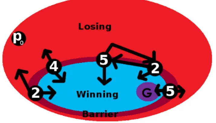
A trace of this algorithm can be found on Figure 1. In 4.4 we prove that pre∗

C(Goal) =

W PC.

4 Theoretical results

4.1 The Problem to Solve

Definition

The initial goal of our problem is to design an eﬃcient algorithm that takes in input a game and returns a winning coalition with the smallest size.

We extend this deﬁnition for every cost function over the coalitions. As a result, the inputs are the game and a cost function cost. Formally, our problem is to ﬁnd C s.t.

C ∈ GW ∧ ∀C′ ∈ GW ⇒ cost(C′_{) ≥ cost(C)}

In the following, the set of cheapest winning coalitions is Coptand a cheapest winning

coalition is Copt ∈ Copt

Where Does the Time Go By?

The problem to check if a coalition of size k can win a given game is NP-complete (as shown in [2]). Let us deﬁne which parts of our problem are diﬃcult to solve polynomially. We manipulate 2 spaces exponential to their representation: the game space and the coalition space.

First, let us focus on the game space. In our case, we restrict to ﬁnite games. Nonethe-less, even in this case, the size of the automaton representing the game can be exponential over the size of its representation. In k rules (transitions deﬁned for a subset of the posi-tions), up 2k _{positions can be expressed.}

For instance, let us deﬁne a 1-player vector-modiﬁcation game. Every location is a binary vector of size k and p0 = (0, 0, . . . , 0). The ith rule sets the ith bit to 1 and every

(10)

rule is triggerable in every position. Trivially, every binary vector of size k can be a position of this game. As there is 2k _{vectors, there is 2}k _positions.

Such representations implies to use specially designed tools that avoids enumerating every position. The tool we used (BDDs) is presented in section 6.2. Moreover, such rep-resentation triggers that algorithms should not enumerate the position-space, restricting the set of algorithms that can be used.

The game must be stored in memory intend to use algorithms on it. This space limit is so a hard constraint.

On this exponential-size space, the space of coalitions added on it is exponential too. As every coalition can be the smallest winning one, the search-space, or the coalition space is the space of partitions of Agt. Its size is equals to 2|Agt|_.

Contrary to what we need for the game representation, there is no real need to store the whole search space. To solve our problem, we can easily enumerate every coalition and test if it is winning one by one. Even if being memoryless is time-consuming, in the algorithms we design, keeping in memory a set that can increases up to the whole search space is intractable.

In this section, we present theoretical foundation needed in our algorithms and data structures. Every piece of theory is linked to its applications and to notes if necessary.

4.2 Winning Transitivity

Coalition space is interesting since it presents this properties:

Property 2 • If a coalition is winning then, every super-coalition is also goal-winning.

• If a coalition is losing then, every sub-coalition is also losing.

Formally, ∀C, C′ _{∈ Coal, C}′ _{⊇ C ∧ C ∈ GW ⇒ C}′ _{∈ GW and, ∀C, C}′ _{∈ Coal, C}′ _⊆

C ∧ C /∈ GW ⇒ C′ _{∈ GW}_/

Proof The proof of ∀C, C′ _{∈ Coal, C}′ _{⊇ C ∧ C ∈ GW ⇒ C}′ _{∈ GW is trivial. If C have}

a winning strategy, then C′ _{have for winning strategy: the same winning strategy than}

the C one for every agent in C ∩ C′ _{and a random one for agents in C}′ _{\ C. As the C}

winning strategy is played then the new strategy is winning for C′_.

The proof of ∀C, C′ _{∈ Coal, C}′ _{⊆ C ∧ C /}_{∈ GW ⇒ C}′ _{∈ GW is symmetrical : if ¯}_/ _C

have a strategy to prevent C to be goal winning, then ¯C′ _{⊇ ¯}_{C have the same winning}

strategy. Consequently C /∈ GW ⇒ ∀C′ _{⊆ C ∧ C}′ _{∈ GW .}_/

Definition 6 A set S of sets is a downward-closed set iff S ∈ S ⇒ ∀S′ _{⊆ S.S}′ _{∈ S. A}

set S of sets is an upward-closed set iff S ∈ S ⇒ ∀S′ _{⊇ S.S}′ _{∈ S.}

The property 2 shows that GW is upward-closed. Oppositely, the set of losing coali-tions is downward closed.

Note that the theory of this property is far more general than game theory. Every problem ruled by a search space with a partial order function over its elements can use these properties and applications.

(11)

4.3 Winning positions properties

Proposition 3 If a position is winning for a coalition, then this position is winning for every bigger coalition. Consequently, the set of winning positions is increasing with the coalition increase. Formally:

(1)∀C ⊆ C′ _{∈ Coal, ∀p ∈ P os, p ∈ W P}

C ⇒ p ∈ W PC′

(2)W PC ⊆ W PC′

Proof The proof is quite trivial and the argument is the same than the one presented in section 4.2: if C have a winning strategy from p then C′ _{have the same winning}

strategy.

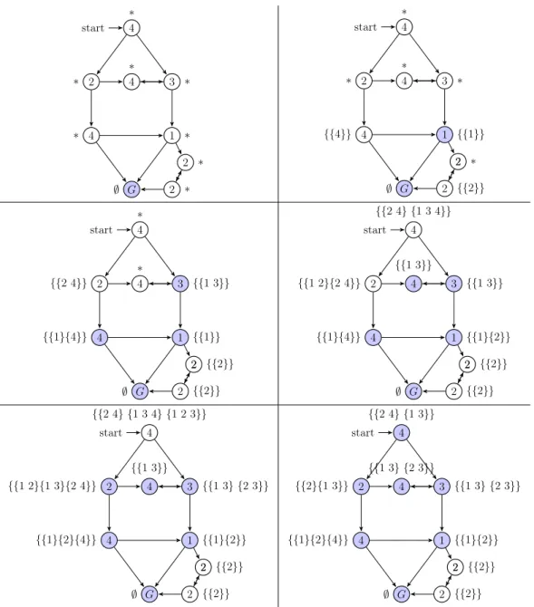
4.4 Barricades

Definition 7 A barricade B for a coalition C is a set of positions s.t. owner(B) ⊆ ¯C and cuts the game (every path from the initial location to a goal contains at least one position in B) in 2 parts: BW and BL (and B ⊆ BL). BL contains no goals and every

position p ∈ B contains a successor in BL, by an action go_back(p).

Proposition 4 Every position p ∈ BL is losing.

Proof In selecting the action go_back(p) for every position in B, ¯C prevents any play from L to reach a goal, so no position in BL can reach the goal. Consequently, every

position p ∈ BL is losing.

Property 5 B = pred(pre∗

C(Goal)) \ pre∗C(Goal) is a barricade for C

Proof For every p ∈ pred(pre∗

C(Goal)) \ pre∗C(Goal), owner(B) ⊆ ¯C is true otherwise p

would be in {p|p ∈ pred(pre∗

C(Goal))∧owner(p) ∈ C}, so p would we in pred(pre∗C(Goal)).

Trivially, any path from a losing to a winning position goes through a predecessor of a winning position, so B is a cut. BL does not contain any goal, otherwise a losing

position would be a goal. Every position p ∈ B contains a successor in BL, otherwise

p ∈ {p|p ∈ pred(pre∗

C(Goal))) ∧ succ(p) ⊆ pre∗C(Goal))} and then p ∈ pre∗C(Goal).

In the remaining B = pred(pre∗

C(Goal)) \ pre∗C(Goal). Let us illustrate a barricade on

the ﬁgure 2.

Corollary 6 BW = pre∗C(Goal) = W PC

Proof pre∗

C(Goal) ⊆ W PC has been proved in section 3.2. pre∗C(Goal) ⊇ W PC : as

B = pred(pre∗

C(Goal)) \ pre∗C(Goal) is a barrier, any position p /∈ pre∗C(Goal) that would

be in BL, so p cannot be winning.

Corollary 7 W PC = W PC∪(Agt\owner(B))

Proof The argument is the same one presented in Propriety 16, but in an iterative point of view. Let us deﬁne by {a1. . . ak} the agents in C ∪ Agt \ owner(B).

In adding a1 the barrier remains the same. This reasoning can be iterated in setting

C to C ∪ a1. Then in adding a2 the barrier still remains the same, and to on.

(12)

Corollary 8 C is losing ⇒ C ∪ (Agt \ owner(B)) is losing.

Proof W PC∪(Agt\owner(B)) = W PC. If C is losing, then p0 ∈ W P/ C then p0 ∈ W P/ C∪a so

C ∪ (Agt \ owner(B)) is losing.

Corollary 9 For any barricade B for a coalition C, Agt \ owner(B)

Proof Let us relax the problem in setting G′ _{= B}

W: if a C have a winning strategy to

reach G then C can use the same strategy to reach G′ _{⊇ G.}

Given this relaxation, let W P′

C be the set of winning positions in this relaxation.

Trivially, B is a barricade for this extended problem (with the same reasons as before). As B is a barricade, agents of owner(B) have a strategy s to prevent C to be goal-winning. In applying s in the original problem, agents in owner(B) prevents C to be goal-winning.

As a result, the coalition C ∪ (Agt \ owner(B)) is losing.

4.5 Overestimate a Biggest Winning Coalition with a Path

Property 10 A winning coalition Cw can be computed from any path ’path’ from p0 to

a winning position. Moreover, Cw = {a|∃p ∈ P os, p ∈ path ∧ owner(p) = a}

Proof This coalition is the set of agents owning a position in the path. As a result, the strategy s that consists in following this path is trivially winning. Formally, ∀1 ≤ i ≤ |path|, (p = path(i)) ⇒ (∃a ∈ Act, s.t.(s(p) = a) ∧ Edg(p, a) = path(i + 1)) is winning. In every position of this path (starting from the p0), the position is owned by Cw and leads

the game to the next position of this path until reaching the goal.

This coalition is not necessarily the smallest one, maybe a smaller coalition (even the empty coalition) can be the smallest winning coalition. This coalition can be not comparable with the inclusion to Cw. Moreover, instead of reaching a goal, the path can

stop on a winning position: from such position there exists a winning strategy leading to the goal.

This method can then be applied to reach a W PC set, in this case the estimation is

Cw∪ C.

4.6 Worst Case

Unfortunately,none of these assumptions can not help us to avoid the worst case. This case is the following: every coalition of size |Agt|/2 + 1 is winning and every coalition of size |Agt|/2 is losing. The cost function is the cardinal cost. In this case, we must (at least) enumerate C_|Agt||Agt|/2 coalitions (coalitions of size |Agt|/2) to test if one of these is winning. Pruning cannot reduce this number of checks, but caching can reduce the check time.

(13)

5 Algorithmic Solutions

5.1 Checkers Optimizations

Cache

We showed in section 11.3 and in section 3.2 that checking algorithms uses eﬃciently sub-estimations of W PC. For every coalition Cs and Cb s.t. Cs ⊆ Cb then W PCs ⊆ W PCb.

We can then cache the W PCs set.

For instance, when computing W PCb, instead of starting from scratch, the W PCs

set can be reused. Instead of computing pre∗

Cb(G) we can compute pre

∗

Cb(W PCs). For

the M inM ax algorithm applied on Cb, when the search reaches a node n = (i, p) s.t.

p ∈ W PCs then this node can be immediately replaced by a W leaf.

In section 6.3 more details are provided on the implementations of this cache.

To keep this cache as minimal as possible without loss of information, the set of com-puted elements evolves dynamically. If every direct super-coalitions of Cs are computed,

then Cscan be removed since if any bigger coalition CB needs an approximation of W PCB

then there exists Cb ⊆ CB and W PCs ⊆ W PCb ⊆ W PCB, so W PCb is a better

approxima-tion of W PCB.

Of course, if the computer runs out of memory, it is possible to safe space in removing item of this cache.

The Cheapest Strategy in a Game

In section 7.2.4 we are interested by games where every action is combined to a price. Let us deﬁne a function costα : Act → R be a cost function for every action. Then,

let us deﬁne the function costp by costp : P lay → R s.t. if pl is not goal-winning then

costp(pl) = +∞ let l be the index of pl s.t. pl(l) ∈ Goal. Then, the cost of this play is

P

i=1..l−1costα(pl(i)a).

Definition 8 A strategy sC is the cheapest strategy for a coalition C, if :

• for any strategy s_C¯ for ¯C s.t. s_C¯ = argmax_{s strategy of ¯}_Ccost(sC ∧ s_C¯),

• for any other strategy s′

C for C and strategy sC2¯ for ¯C s.t. sC2¯ = argmaxs strategy of ¯Ccost(sC∧

s_C2¯ )

then costp(sC ∧ s_C¯) ≤ costp(s′C∧ sC2¯ ).

There is diﬀerent ways to compute the cheapest strategy for a coalition C in a game with a cost on every action. The simplest one is to add payoﬀs on the M inM ax search. Then αβ pruning optimizations can be used to remove prematurely useless branches.

Here we propose a variant of the pre∗

C(G) algorithm, because this algorithm has proven

its performances over M inM ax without heuristics. Similar algorithms exists to compute optimal value in stochastic games like in [5], [4] or for Markov Decision Processes [9]. The principle consists in storing the best cost for every position in a map m : P os → R and updating this value until reaching a ﬁx-point thanks to this process: m0 _{:= {p ∈ Goal ⇒}

0, others ⇒ +∞} m is updated at every iteration by this process : the cost c of every position p s.t. owner(p) ∈ C is: c = argminα∈Actcostα(α) + m(Edg(p, α)). Reciprocally

(14)

m ← {g ∈ Goal ⇒ 0, others ⇒ +∞}; repeat

foreach Position p ∈ P os do if owner(p) ∈ C then

m(p) ← argminα∈Actcostα(α) + m(Edg(p, α));

else

m(p) ← argmaxα∈Actcostα(α) + m(Edg(p, α));

end end

until m has not converged ;

Algorithm 1: the cost of the cheapest strategy in an game with costful actions

if p ∈ ¯C, c = argmaxα∈Actcostα(α) + m(Edg(p, α)). This algorithm updates the values

until reaching a ﬁx-point. This speciﬁcation is described by the algorithm 1.

More details about the symbolic implementation of this algorithm are discussed in section 6.5.

5.2 Coalition-Based Seeker

Introduction

In this section, we present an algorithm that looks for the cheapest winning coalition in searching the coalition-space. In using a checker (presented in section 3) this algorithm checks winning and losing coalitions intend to compute the cheapest winning one: Copt

As we manipulate huge games, every checking operation is costful (and empirically, the time of every check for the same game is constant). Our objective is to look for the best coalitions to check, intend to get the cheapest winning coalition with a minimal number of checks.

Let us deﬁne the structure we manipulate in this framework: • Comp ⊆ Coal the set of checked coalitions

• GWe⊆ GW the estimation of the winning coalitions

• Lose⊆ ¯GW where ¯GW = {C|C /∈ GW }, the estimation of losing coalitions

• U nke= Coal \ Lose\ GWe be the set of unknown coalitions

• Let Copte ∈ GWe be the estimation of the cheapest winning coalition

A simple way to solve our problem is to check every C ∈ Coal and then Copte is the

cheapest winning coalition. To enhance performances, we used some theoretical properties to avoid such useless computations.

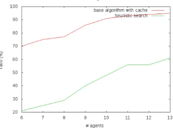
There are different ways to explore the coalition space, so we defined simple functions to explore it. In annexes 11.4 we present the tool we designed intend to enhance per-formances of the search, by allowing more subtle comportments. In our data-sets, such specialized tools were less efficient than the following basic search.

The search ends when mc(Copte) \ Lose = ∅, then Copte = Copt. mc is deﬁned in section

(15)

Definition 9 A check of a coalition C is useless if C is checked and exists a coalition C′

s.t. C′ _{⊂ C,C}′ _{∈ GW and C}′ _{is checked, or exists coalition C}′ _{⊃ C, C}′ _{∈ GW andC}_/ ′ _is

checked

This deﬁnition is linked to the cache operation, presented later.

Formal Definition of the Coalition-Based Search

Given these deﬁnitions, let us deﬁne formally the problem. Let OptCoal ⊆ 2Coal _{be the}

set of sets of coalitions coalitions s.t. for any Calc ∈ OptCoal, in checking any coalition C ∈ Calc:

• exists an optimal coalition Copt s.t. Copte = Copt

• mc(Copte) \ Lose= ∅

The problem is to compute OptCalc ∈ OptCoal s.t. |OptCalc| is minimal.

In our case, we restrict to an approximation of this minimum. Let us note that OptCalc

have no useless checks.

Pruning

In section 4.2, we showed that: ∀C ∈ Coal, ∀C′ _{⊇ C, C ∈ GW ⇒ C}′ _{∈ GW and}

∀C ∈ Coal, ∀C′ _{⊆ C, C /}_{∈ GW ⇒ C}′ _{∈ GW}_/

As a result, each time a coalition C is checked, we can

• remove from U nke and add to Lose the set: {C′|C′ ⊆ C} if C is losing

• remove from U nke and add to GWe the set: {C′|C′ ⊇ C} if C is goal-winning

This property allows to prune a lot of coalitions in very few checks (the maximal bound is given in section 11.6). The most famous example is in a game that cannot be won. In checking only the coalition Agt (that is losing), we can prune the whole state-space, since every smaller coalition is losing.

Definition 10 A check of a coalition C is useless a priori (resp. a posteriori) if C is computed in an iteration i there exists i′ _{< i (resp. i}′ _{> i) s.t. a coalition C}′ _{⊂ C and}

C′ _{∈ GW is checked in the iteration i}′ _{or a coalition C}′ _{⊃ C and C}′ _{∈ GW is computed}_/

in the iteration i′_.

Then, a check of a coalition C is useless a posteriori C is pruned by C′_{, so in permuting}

the checking order C would not have been checked (because useless a priori ).

In the following we extend the checkers s.t. when a coalition C is checked, either: • C ∈ GWe or C ∈ Lose then no check is necessary and the correct value can be

returned immediately

• C ∈ U nke then a set GWe or Lose is updated thanks to this check.

(16)

Barricade

Barricades are deﬁned in section 4.4. Immediately from the corollary 8, given W PC, if

C /∈ GW , then C ∪ (Agt \ owner(pred(W PC) \ W PC)) /∈ GW . In computing only for

the predecessors of W PC, we can add to GWe a bigger coalition than C. Let B be this

barricade.

Then, thanks to the corollary 9, any other barricade B′ _{allows to prune C ∪ (Agt \}

owner(B′_{)). We used pre}∗

C(Goal) to compute W PC. To detect another barricade, we

simplify the problem like in the proof of the corollary, by adding B to the set of win-ning positions. Then we iterate on : pre∗

C(pre∗C(Goal) ∪ B). Once again, if p0 ∈/

pre∗

C(pre∗C(Goal) ∪ B), we can iterate on pre∗C(preC∗(pre∗C(Goal) ∪ B) ∪ B′) where B′ =

pred(pre∗

C(pre∗C(Goal) ∪ B)) \ pre∗C(pre∗C(Goal) ∪ B) and so on.

Because of the add of every position of the barricade in the W PC set, a position p s.t.

next(p) ⊆ B, owner(p) ∈ ¯C and |owner(next(p))| ≥ 2 is in pre∗

C(pre∗C(Goal) ∪ B) but

could not be winning in buying only one agent. As a result, the number of barricades found by this algorithm is not an upper bound of the agents needed for victory. Moreover, some agents, not appearing in any barricade can be needed for victory like p for instance. This optimization is not used in practice, since this check is as costful as a complete search of the pre algorithm and the pruning factor is not suﬃcient in our games to be interesting.

Getting a Maximal Losing/Minimal Winning Coalition

In section 11.6 we evaluate the maximal number of coalitions that are pruned in every check. There, we show that the bigger a losing coalition or the smaller a winning coalition is the more eﬃcient is the pruning. As a result, computing the maximal losing coalitions or minimal winning coalitions prunes heavily the search space.

The algorithm 2 presents how to compute a maximal losing coalition given a losing coalition C. Note that a symmetrical algorithm exists to search of a minimal winning coalition.

Input: C: losing coalition

Output: Cm: maximal losing coalition

Cm ← C;

foreach Agent a from Agt do if Cm∪ a is losing then

Cm ← Cm∪ a;

end end

return Cm

Algorithm 2: Maximal Losing Coalition

Property 11 Invariant : Cm is losing.

Proof In the ﬁrst iteration Cm = C and C is losing. For every iteration, a is added to

(17)

Property 12 Cm is a maximal losing coalition.

Proof Let us prove that Cm is maximal. Let us suppose that Cm is not maximal, then

a coalition C′

m s.t. Cm ⊂ Cm′ . So there exists an agent a ∈ Cm′ and a /∈ Cm. There is an

iteration where a coalition Csubm ⊆ Cm checks Csubm∪ a and do not add a, so Csubm∪ a

is winning. Or Csubm ⊆ Cm, so Csubm∪ a ⊆ Cm∪ a ⊆ Cm′ .

Thanks to the property 2, as C′

m is losing, then every of its sub-coalitions are losing,

or Csubm∪ a is one of its sub-coalitions and is winning. So, Cm′ cannot exist and Cm is a

local maximal losing coalition.

Trivially, the complexity of this algorithm is |Agt| ∗ δc where δc is the complexity of the

checker used. Let us recall that empirically δc is roughly constant. Moreover, the cache

(presented in 5.1) is extremely well used in this setting because agents are added 1 by 1. Let us note that the order agents are selected is not fixed. In selecting different orders, it is possible to get different maximal losing coalitions. The best case is to get losing coalition with the biggest cardinal.

A variation of this algorithm is proposed in annexes 11.9.

The Main Algorithm

In this algorithm we look for the cheapest winning coalition. We showed that if mc(Copte)\

Lose = ∅ then Copte is a cheapest winning coalition.

As a result, given an estimation of Copte, is computing every C ∈ mc(Copte) we can

prove either that Copte is winning (if every C ∈ mc(Copte) is losing), either there exists

C ∈ GW and C ∈ mc(Copte). As cost(C) < cost(Copte) then Copte can be updated by C,

until reaching the minimal value.

We showed that in checking the maximal losing coalitions, we often prune a far more coalitions in general and in mc(Copte) than in checking elements than mc(Copte). Moreover,

let max be the set of maximal coalition, practically often |M ax| ≤ |mc(Copte)|. Let us

present the search process in algorithm 3.

Proof • Termination: In every iteration of the while loop, to_test checks a coalition C ∈ Coal:

– either to_test is updated, then C ∈ GW , then Copte is updated by C and

cost(Copte) decreases. As the cost is aﬀected to a coalition and the set of

coalitions is ﬁnite, the set of costs is ﬁnite. As cost(Copte) decreases when

updated by C, then the number of updates of to_test is ﬁnite

– either to_test is not updated, then C is a losing coalition and C /∈ U nke. After

the iteration at least C is removed to U nke. As Coal is ﬁnite, the number of

checks is ﬁnite.

• Correctness: Les us show that Copte = Coptis trivial from the deﬁnition of mc(Copte).

If no coalition from mc(Copte) is winning then Copte ∈ Copt.

The mc operator is capital because it contains unknown losing coalitions like Cu. Cu

(18)

Output: Cheapest winning coalition if check(Agt) is losing then

return null else

Copte ← Agt

end

to_test ← mc(Copte);

while there exists a coalition C ∈ (to_test ∩ (U nke∪ GWe)) do

if check(C) then Copte ← C; to_test ← mc(Copte); else remove_maximal_losing_coalition_f rom(C); end end return Copte

Algorithm 3: The coalition-based seeker

As a result, any call of remove_maximal_losing_coalition_f rom(C) removes a new maximum. Moreover, this call prunes (at least one) element of to_remove. A trace of the execution of this algorithm is presented in section 11.1

Complexity

In section 5.2 that, given a losing coalition, a maximum can be found in |Agt| checks. Let δc be the check complexity.

Let δmc be the complexity to get an unknown or winning element from the mc set.

Let us note that this complexity is linear on Coal for every of our cost functions. The complexity of this search algorithm is so :

|M ax| ∗ |Agt| ∗ (δc+ δmc)

Let us note that in the worst case (presented in 4.6), |M ax| = Cnn/2.

5.3 Position-based Algorithm

This seeker is a kind of dual of the based resolution process. In the coalition-based method, we compute the W PC set, in this approach, we compute the winnersp

set. As a result, winnersp0 = GW . We no not actually compute the smallest winning

coalition but the GW set. Once done, we can know if C is winning in O(|Agt|) instead of O(δc) (where δc is the cost of a check).

Let us present the main idea. In every position p, either: • we buy the owner(p), so a p′ _{∈ next(p) must be winning}

(19)

The algorithm updates the winnersp set for every position p where winnersp

repre-sents the set of winning coalitions from p. Let us call winners0

p be the initialization and

winnersi

p obtained after i iterations. Let us present the updating process:

winnersi+1_p =

winnersi_p [

(a){C ∪ owner(p)|∃p′ ∈ next(p), C ∈ winnersi p′}

[

(b){C|∀p′ ∈ next(p), C ∈ winnersi_p′}

(1)

A trace of the execution of this algorithm is presented in Figure 1. Property 13 For every i, C ∈ winnersi

p ⇔ p ∈ preiC(Goal)

Proof We proceed by induction over i.

i = 0 : for every coalition C ∈ Coal and every position p ∈ P os, if p ∈ Goal then p ∈ pre0

C(Goal) = Goal and C ∈ winners0p = Coal, else p /∈ pre0C(Goal) and

C /∈ winners0 p = ∅.

Let us suppose this property true for the iteration i, let us prove that this property is true for the iteration i + 1.

• C ∈ winnersi+1

p ⇒ p ∈ prei+1C (Goal):

– if C ∈ winnersi

p then by hypothesis p ∈ preiC(Goal), as preiC(Goal) is

increas-ing, p ∈ prei

C(Goal)

– C /∈ winnersi

p (and C is added into winnersi+1p )then:

∗ by (a): C ∈ {C′ _{∪ owner(p)|∃p}′ _{∈ next(p), C}′ _{∈ winners}i

p′}. Let p′ ∈

next(p) s.t. C′ _{∈ winners}i

p′. Trivially C′ ∈ winners_p′, then C ⊇ C′ ∈

winnersp′. Then, by hypothesis, as p′ ∈ prei

C(Goal) and p ∈ pred(p′),

then p ∈ {p|p ∈ pred(prei

C(Goal)) ∧ owner(p) ∈ C} so p ∈ prei+1C (Goal).

∗ by (b): C ∈ {C|∀p′ _{∈ next(p), C ∈ winners}i

p′}. Then as C is in

ev-ery p′ _{∈ next(p), C ∈ winners}i

p′. By hypothesis, every p′ ∈ next(p) ∈

prei

C(Goal), then p ∈ {p|p ∈ pred(preiC(Goal)) ∧ next(p) ⊆ preiC(Goal)}

so p ∈ prei+1_C (Goal). • C /∈ winnersi+1

p ⇒ p /∈ prei+1C (Goal).

– If owner(p) ∈ C then, for every p′ _{∈ next(p), C /}_{∈ winners}i

p′ (otherwise C

would have been added to p by the rule (a)). Consequently for every p′ _∈

next(p), p′ ∈ pre/ i

C(Goal). Consequently, no successor of p is in preiC(Goal),

then p /∈ prei+1_C (Goal)

– If owner(p) /∈ C then exists p′ _{s.t. C /}_{∈ winners}i

p′ (otherwise C would have

been added to p by the rule (b)).

Consequently, owner(p) /∈ C and next(p) ⊆ prei

C(Goal) is false, so p /∈

(20)

Corollary 14 For every position p, winnersp converges to the set of the winning

coali-tions in every p.

Proof Immediate from the lemma 13.

6 Implementation Aspects

6.1 Frontiers

Frontiers are used to represent (downward or upward) closed sets. Formal deﬁnition are given in 6. Such sets are frequently used to represent the coalition space (in both the coalition and the position based algorithms), thanks to the properties of 4.2.

For simpliﬁcations purposes, we focus on downward-closed frontiers, since upward-closed frontier are symmetrical.

Let us deﬁne by S the set of set to be represented. In this section, sets of sets are represented in bold and sets in capital letters.

Let us call F ⊆ S the frontier represented.

Exhaustive Implementation

In this naive implementation, every S is exhaustively conserved in F. Then, each time a set S, every S′ _{⊆ S is added to F. Of course, this implementation intractable: for the}

search space frontier F rise up to |Coal|.

Nonetheless, with an eﬃcient hash function, this implementation allows to compute eﬃciently S ∈ F

Symbolic Implementation

Instead of manipulating exhaustively every S ∈ S, we manipulate only a least representa-tive subset Sm. Sm is the set of maximal sets of S. Formally, S ∈ S ⇔ ∃S′ ∈ Sm, S ⊆ S′.

To add S in S: let us update Sm s.t. (Sm\ {S′|S′ ∈ Sm∧ S′ ⊂ S}) ∪ S. To test if S

in S, it is suﬃcient to test for every Sm ∈ Sm if S ⊆ Sm.

In this case, these operations have a complexity in O(|Sm| ∗ |Agt|).

For the search-space, in the worst case (in section 4.6), |Sm| can increase up C |Agt|/2 |Agt|

but no more. In this case, every coalition is either a sub-coalition or a super-coalition of a coalition of this border.

We present in section 6.2.4, how to use symbolic structures to represent Sm. In

ap-plications, s.t. the position-based algorithm (in section 5.3, this kind of representation dramatically enhance performances. Note that for symbolic sets, such frontier can repre-sent in a single BDD upward and downward closures.

Let us note that with a symbolic representation using a BDD, the complexity to test a coalition is O(|Agt|), and to add a new agent O(|Sm| ∗ |Agt|2) (the product of the sizes

(21)

6.2 Symbolic Representations of Structures

In this section we present incrementally how to design a transition system and to manip-ulate it with a symbolic representation.

Such symbolic representations can be implemented eﬃciently thanks to a BDDs. Lots of applications uses this feature, like [3] or [10].

6.2.1 Minimal Representations and Operations

First, let us consider symbolic representation of simple objects.

Let V ars be an ordered set of variables. Let F orm be the set of propositional formulas with variables from V ars. Let Obj be the set of objects we want to represent by a formula. Let us introduce a function code : Obj × 2V ars _{→ F orm. The use of Obj allows to}

overload this function for the diﬀerent objects we manipulate.

Let us deﬁne a reverse function decode : F orm × 2V ars _{→ Obj, s.t. for every O ∈}

Obj and every V ∈ 2V ars_{, O = decode(code(O, V ), V ) and for every F ∈ F orm, F =}

code(decode(F, V ), V ).

Let us deﬁne nb_vars : O → N be the number of variables needed to code/decode an object O. In the following, we suppose that |V | = nb_vars(O).

We precise that if O ∈ Obj is not a set, |V | = nb_vars(O) and F = code(O, V ) then, in our deﬁnitions of code, F have a unique model MF ⊆ V . We extends naturally decode

to decode : 2V _{× V ars → Obj, where decode(F, V ) = decode(M}

F, V ). If F have more

models, decode is extended to : decode : 2V _{× V ars → 2}Obj_{. This function is detailed with}

the set operations.

Let us deﬁne a function swap_variables : F orm × V ars∗_{× V ars}∗ _{→ F orm.}

swap_variables(F, LV, L′V) is deﬁned if |LV| = |L′V|, if for every v ∈ LV then v /∈ L′V

and v have only one occurrence in LV. Then F′ = swap_variables(F, LV, L′V) if the

formula F where every occurrence of vi = LV(i) is replaced by vi′ = L′V(i).

First, let us present code : {0, 1} × 2V ars _{→ F orm, encoding a bit value b with the}

variables V . nb_vars(b) = 1, let V = {v}. code(b, V ) = v if b = 1 else code(b, V ) = ¬v. Reciprocally, if F have one unique model MF, decode(F, V ) = 1 if MF ∩ V = {v},

decode(F, V ) = 0 if MF ∩ V = ∅, otherwise the formula can represent both or none bits

value, cannot be the code of a single value but of a set.

Then, let us represent the pairing operation: pair : Obj × Obj → (Obj × Obj) the well-known operation pair(a, b) = (a, b).

Let us deﬁne the code of a pair. We suppose that the codes of the 2 objects O, O′ _{∈ Obj}

are disjoint, so their sets of variables V, V′ _{⊆ V ars is s.t. V ∩ V}′ _{= ∅. We extend code}

to code : (Obj × Obj) × (V ars × V ars) → F orm. code((O, O′_{), (V, V}′_{)) = code(O, V ) ∧}

code(O′_{, V}′_).

Let us present the reverse decoding operation. In a same way, we extend the decode operation to: decode : F orm × (V ars × V ars) → (Obj × Obj) with the same setting: decode(F, (V, V′_{)) = (decode(f irst(F, (V, V}′_{), V )), decode(second(F, (V, V}′_{), V}′_))).

Let us deﬁne f irst : F orm × (V ars × V ars) → F orm by the natural extension to the f irst operation to F orm domain. f irst(F, (V, V′_{)) = ∃}

v /∈Vv.F . Idem for second:

second(F, (V, V′_{)) = ∃}

v /∈V′v.F .

As V and V′ _{do not shares any variable and the code operation apply the ∧ operator}

(22)

code(O′_{, V}′_{), (V, V}′_{)) = ∃}

v /∈Vv.(code(O, V ) ∧ code(O′, V′)) = code(O, V ). This property is

symmetrical for second.

Note that, given a the bit representation and the pairing operation, we can repre-sent the inﬁnite tape of a Turing machine. So, every data structure can be reprerepre-sented thanks to these minimal formulas. Let us add more power and expressiveness to this representation.

Let us note that the pairing operation extends easily to the tupling operation. With similar reasoning we can get the ith _{projection of a tuple.}

Let us extend this representation to integers from a ﬁnite subset I ⊆ N and exists k s.t. for every 0 ≤ i ≤ 2k_{, i ∈ I. Let B}

n be the binary representation of n ∈ I. Let us

represent Bn by a ﬁnite set on integers s.t. Pi∈Bn2

i _{= n. Trivially,to represent i ∈ I,}

nb_vars(i) = k, let V = {v1. . . vk}. Then, code(n, V ) = (∧i∈Bnvi) ∧ (∧i /∈Bn¬vi). Let MF

be the model of F on V . decode(F, V ) =Pvi ∈ MF2i.

Note that the size of the representation of the elements of I is logarithmic on |I|.

6.2.2 Automaton Objects Representations

These transformations allows us to represent positions of a game. Independently of the games, our positions are tuples: (Int × P rop × · · · × P rop), where Int is an integer value from a ﬁnite set and P rop is a bit value representing a proposition of the game. More details about positions are described in section 7.1. Some positions are a tuple of positions, so still can be represented thanks to our formalism.

Actions and agents are coded by integers (from a ﬁnite set). A transition t is a triple (p, act, p′_{) where p is the starting position, act the action played and p}′ _{the resulting}

location.

We manipulate during this report a symbolic representation of the automaton thanks to transitions. In order to simplify representations, we allocate to different objects of the automaton different variables. Let us define these sets now, given a transition (p, act, p′₎

• Vagt ⊆ V ars for the agent playing in the starting position p. Symmetrically for the

ending position p′_{: V}′

agt⊆ V ars.

• Vprop ⊆ V ars for the status of propositions in the starting position. Symmetrically

V′

prop for the ending position.

• Vp = Vprop∪ Vagt for the starting position p. Symmetrically, Vp′ = Vprop′ ∪ Vagt′ for p′.

• Vact for the action act, in the transition.

• Vtrans = Vprop∪ Vprop′ ∪ Vagt for the whole transition function.

• VCoal for the sets of coalitions of the frontiers (see section 6.1 for more details).

Given the deﬁnition, let us present how to generate a game through an example for the STRIPS games. In section 7.1.2, we present an extension of STRIPS for games. We show here how to generate a symbolic representation from such representation. The algorithm 4 present the method to generate such game. To avoid confusion, a STRIPS action is called a rule. Intend to simplify the construction, let the set of propositions pre of STRIPS be the set Vprop be equals and add, rem be the same propositions than the set Vprop′ .

(23)

Output: T:Transition Function T ← ∅ ;

foreach Rule r = (pre, add, rem, owner, next) do T ← T ∨ ((∧v∈prev) ∧ (∧v∈addv) ∧ (∧v∈rem¬v) ∧ (∧v′

i∈(add∪rem)/ (vi ⇔ v

′ i)));

end

Algorithm 4: Generator of a transition function of a multi-agent STRIPS

In this symbolic representation, if the preconditions are met in the starting location, the resulting location have its add propositions true and rem propositions false. Other propositions are unchanged.

Given such game, let us deﬁne symbolically how to get easily simple symbolic repre-sentation of interesting sets. For instance, get the predecessors of a set of locations is a useful problem (as presented in sections 3.2, 11.5 or 5.2).

Given a set of positions SP, let FSP = code(SP, V

′

p), FT = code(T, Vtrans), the symbolic

representation of the set of predecessors of SP is : Fpred = ∃v∈(Vact∪Vp′)v.FT ∧ FSP

Given Fpred, the representations of biggest subset of pred s.t. owner(pred) ⊆ C is

obtained by : Fpred∧ code(C, VCoal).

In section 11.5 we are interested by the smallest path from p0 to a set of position

P ⊆ P os We proceed in computing a level graph like in an optimization of the well-known Ford-Fulkerson algorithm.

This graphs split the game into n disjoints sets S1. . . Sn. For every position p ∈ Si

the shortest path from p0 is a path of size i. Then, the distance d = mini∈NSi∪ P 6= ∅ is

the minimal distance between p0 and P . Then, a shortest path is a path s.t. (p0, . . . , pd)

s.t. pi+1 ∈ next(pi), pi ∈ Si and pd ∈ P . Thanks to the deﬁnition of the level graphs,

such path exists.

In this section, we showed how to represent symbolically objects of a game. Then, we presented how to generate a game from a symbolic description and some basic operations over this game.

6.2.3 Sets Representation and Manipulation

Symbolic representations are extremely eﬃcient to represent compactly sets with simi-larities between its elements. Let us present the basic set operations : generating the empty-set, generating a singleton, union, intersection and complement).

Let S, S′ _{be 2 sets whose objects can be represented thanks to the same variables V .}

Let us deﬁne the basic set operations in a symbolic setting: • code(∅, V ) = ⊥

• code({O}, V ) = code(O, V )

• code(S ∪ S′_{, V ) = code(S, V ) ∨ code(S}′_{, V )}

• code(S ∩ S′_{, V ) = code(S, V ) ∧ code(S}′_{, V )}

• code(S \ S′_{, V ) = code(S, V ) ∧ ¬code(S}′_{, V )}

(24)

• The test O ∈ S is equivalent to test code({O} ∩ S, V ) = code(∅, V )

Let us note that ⊤ have every model in V , then ⊤ is the set of every elements O that can be expressed on V . This note let us extend the representation to symbolic sets.

Let us consider the following example, manipulating a set of transitions T , we want to add the constraint “player 2 plays always and only after player 1”.

Let us code the player 1 as the starting position player: Fa1 = code(a1, Vagt). Idem for

player 2 as ending position player : Fa′

2 = code(a2, V

′ agt).

Then: T ∧ (Fa1 ⇔ Fa2) codes for this new transition system. Every transition t s.t.

agent 2 is not the successor of the agent 1 does not satisfy this new formula that is T . t have no model, so t /∈ decode(T, Vtrans).

6.2.4 Closed Sets of Sets Representation

Closed sets of sets are used in section 6, section 5.1 and in section 5.3. The symbolic representation of such sets highly improved the performances of our tool. Let S be the set of objects we manipulate and S = 2S _{be the set of set. To represent such sets of sets,}

we represent Ss ∈ 2S by a vector of the elements of S. So, for instance, let S = {a, b, c}

and Ss ∈ 2S s.t. Ss = {a, c} then we represent the set Ss in the variables {va, vb, vc} by

the vector {va= 1, vb = 0, vc = 1}.

Manipulation of symbolic sets of sets is presented in [11]. In our case we are interested by closed sets, this problem have been discussed for data mining purposes in [16].

Let us deﬁne the variables VS ∈ V ars s.t. |VS| = |S|. For every s ∈ S there exists a

unique vs. Let A ⊆ S, let us represent code(A, VS).

• We redeﬁne code : S × 2V ars_{→ F orm by code(S}

s, VS) = (∧s∈Ssvs) ∧ (∧s /∈Ss¬(vs))

• code(∅, VS) = ⊥

• The test Ss ∈ A is equivalent to test code(Ss, VS) ∧ code(A, VS) = ⊥

• Add an upward closed set Su: Au = code(A, VS) ∨ (∧s∈Suvs). Any evaluation of set

Ss ⊇ Su have valuation MSs ⊇ {vs|s ∈ Su}, so Ss∈ Au

• Add a downward closed set Sd: code(A, VS) ∨ (∧s /∈Sd¬(vs))

• Union and intersection set operations have the same code function than the sets. The complementary operation is trickier and not proposed.

It is important to note that a set Ss ⊆ S have 2 possibles codes: one to represent a

traditional sub-set of S and one to represent a closed element of S and cannot be mixed. This closed set of set representation improves time and space mean-time during the execution. Because of a bug in the Java BDD-interface we get, we could not test the eﬃciency on ZBDDs like authors in [16] do.

(25)

6.3 Cache

The cache Cache, presented in section 5.1 stores a subset of W PC during the checking a

operations.

A ﬁrst implementation of this cache is done with a map operation. The problem is that, given a coalition C, we would like to get [

C′_⊆C

W PC′. Unfortunately, getting coalitions for

every subsets is intractable. Some solutions, more eﬃcient, consisted in testing only the direct sub-coalitions of C, adapting the search using this fact (in adding agents one by one). Moreover, as the set of computed coalitions remains empirically small, it is possible to test for every coalition in Comp if this coalition is a subset of C or not.

Nevertheless, in storing symbolically the cache, with same representation than in the position-based algorithm (presented in section 6.4), we can more get more eﬃciently the cache. In this representation, Cache is deﬁned by: Cache ⊆ 2Coal×2P os

. Then CacheC =

∃vi∈VCoal.(Cache ∧ code(C, Vcoal)).

Let us note that for the BDD representation, variable ordering is extremely important for performances purposes (as presented in [20]). Our BDD interface allowed us to select eﬃciently a good variable ordering.. We do not detail here the use of BDD variable ordering, but oppositely to the position-based algorithm, Vcoalition must have a smaller

value than Vpos, intend to keep correct performances.

6.4 The Position-Based Algorithm in a Symbolic Structure

In this implementation, we update the map winners : position → Coal, given the propo-sition presented in section 5.3. In symbolic setting, this map can be confused with a set.

In every iteration, Then, we combine these successors with T to get the set M : starting × ending × coalitions. Depending on the rule applied, application, we can get C or ¯C predecessors with an and operation on M with the BDD representing C or ¯C. Other operations are less relevant to our application.

The position-based algorithm is presented in algorithm 5.

6.5 Computing a Cheapest Strategy

In section 5.1 we presented an algorithm that computes the cheapest strategy s for a coalition C in a game. The problem is that the cost of every position must be exhaustively enumerated, which is intractable. Fortunately, some algebraic data structures are designed to handle such graph problems with eﬃciency (for instance the algorithm used in [9] can handle million of states).

These structures are similar to symbolic propositional formulas, but for every evalu-ation of this formula is not ⊤ of ⊥ but a value from a set of constants Q. The exact deﬁnition given in [1], let us simplify it by: a formula f is an algebraic formula from a set of variables V if f is a function f : {0, 1}|V | _{→ Q.}

An ADD is a data structure that represents eﬃciently such formulas where Q = R, peculiarly for graph or matrix operations. In few words, ADDs are a data structure very similar than BDDs, but, instead of associating leafs by ⊥ and ⊤, leafs are associated to real values.

(26)

Input: G:game

Output: Set of winning coalitions

winners ← {(goal ⇒ ⊤), (others ⇒ ⊥)}; repeat winners′ _{← swap_variables(winners, V} p, Vp′); winning_coalition_and_predecessors ← T ∧ winners′_; buy_agent ← winning_coalition_and_predecessors; buy_agent ← ∃v∈(V′ p∪Vact)v.buy_agent;

%buy_agent, is a map p → {winnersp′|p′ ∈ next(p)}

foreach Agent agt do

buy_agent ← buy_agent∧(code(agt, Vagt) ⇒ (code(agt, Vcoal)∧buy_agent));

end

%buy_agent is a map p → {winnersp′ ∪ owner(p)|p′ ∈ next(p)}

winning_coalitions_by_action ← ∃v∈V′

pwinning_coalition_and_predecessors;

%winning_coalitions_by_action, is a map %p × Act → {winnersp′|p′ ∈ Edg(p, a)}

buy_successors ← ⊤; foreach Action act do

buy_successor_by_a ←

∃v∈Vactv.(winning_coalitions_by_action ∧ code(act, Vact));

%buy_successor_by_a is the map %p → winnersEdg(p,a)

buy_successors ← buy_successors ∧ buy_successor_by_a; end

%buy_successors is the map %p → \

a∈Act

winnersnext(p)

winners ← winners ∨ buy_successors ∨ buy_agent; until the fix-point for winners is reached ;

return winnersp0

(27)

• The boolean operation is the traditional ite applied on ADDs, where ⊤ is replaced by 1 and ⊥ by 0. Other traditional propositional logic operators can then be deﬁned. • Arithmetic operations: (+, −, min, max . . . ). Apply(f, g, op) is equivalent to

asso-ciate the algebraic formula h, s.t. for every valuation of V = {(0, . . . , 0), (0, . . . , 1), . . . , (1, . . . , 1)} the algebraic formula h = {(0, . . . , 0) → op(f (0, . . . , 0), g(0, . . . , 0)), (0, . . . , 1) →

op(f (0, . . . , 1), g(0, . . . , 1)), . . . , (1, . . . , 1) → op(f (1, . . . , 1), g(1, . . . , 1))}

• Variable abstraction: such abstraction remove a variable by abstracting it (like the ∃ and ∀ operators do in formulas. Let us restrict to closed and commutative operators applied on variables 1 by 1 (some speciﬁcations allows to apply operators on sets of variables, causing problems of associativity). Let us call absop

v such operator of

abstraction. Let us deﬁne the substitution operation of a formula F : Fv←F′ is F

where every occurrence of v is replaced by F′_{. Then, abs}op

v (F ) = op(Fv←⊤, Fv←⊥).

The implementation we propose is a variant to the one proposed on [9], which is eﬃcient even on gigantic state-space. The generic algorithm is presented in algorithm 1 and in algorithm 6 we propose the variant for symbolic structures.

Let T be the transition function of the game, represented with to a BDD. Let ADDgen :

BDD × R × R → ADD be an function s.t. ADDgen(b, v1, v2) is b where v1 replace the ⊤

node and v2 replace ⊥ node.

The function swap_variables is extended for ADDs with the same deﬁnition than the function for BDDs presented in section 6.2.1

This algorithm can be extended to the position-based way: it is possible to compute, for every position p, the cost of every coalition. This idea could not implemented since our ADD library was a too much time-consuming and to our knowledge, no ADD library are implemented nor interfaced for Java.

Let us note that such technique allows the use of a cache. For every C′ _{⊇ C, let}

mC (resp mC′) be m for C (resp. C′), then for every position p, m

C(p) ≥ mC′(p). So

instead of starting computing mC from scratch, mC can be initialized for every p by

mC(p) = min(mC1(p), . . . mCk(p)) for every Ci ⊆ C

7 Discussion on Games and Costs

7.1 Games

7.1.1 Autistic Games

These games have been designed to test our software. Every agent plays “autistically” front of her own solo-game without interacting with someone else. Agents plays circular order.

These games are convenient to set the winning coalition in by setting for goal “every agent reaches its solo-game goal state”. As agents do not interact, every agent that can choose to win or lose in its solo-game must be added to the winning coalition. Oppositely, if a agent plays a game automatically wins, no matter what she plays, then she is not needed in the minimal coalition. By her actions, she cannot prevent the game to win, even if she is an enemy.

(28)

Input: G : Game, C : Coal

Output: Cost of a cheapest strategy of C next_cost ← (g ∈ Goal ⇒ 0, others ⇒ +∞); foreach Action act do

trans ← ∃v∈Vact∪VAgtv.T ∧ code(act, Vact);

% trans is the transition function when act is selected Qact← ADDgen(trans, cost(act), 0);

end

%Qact is the cost to add to m(p) when act is played in p

repeat

m ← next_cost;

onlyC ← ADDgen(code(C, Vagt), 0, +∞);

only_C¯ ← ADDgen(code( ¯C, Vagt), 0, −∞);

foreach Action act do

costact← Qact+ next_cost;

%costact: p → R is cost from p if a is played

costact,C = costact+ onlyC;

costact, ¯C = costact+ only_C¯;

% if owner(p) ∈ ¯C then costact,C = +∞

end

next_cost ← costact;

%let next_cost be a selection of an action foreach Action act do

next_cost ← max(next_cost, costact, ¯C);

next_cost ← min(next_cost, costact,C);

%as costact, ¯C(p) = −∞ or next_cost, costact,C = −∞ then in one min/max

%operation, next_cost(p) is selected, the ordering of these operations is not %important

end

until m has not converged ; return m

(29)

These games are interesting to present some synchronization problems. For instance, if we have a set of independent processes that terminate only if they all simultaneously enters in a conﬁguration.

Our framework allows to answer problems like: “which systems do we need to control in order to terminate, or how can we shorten the execution by adding more agents or which is the best compromise?”

Nonetheless, this games may look too specific to generate general heuristics. For the objective presented higher, in defining a goal where everyone must win hers local game, they is only one minimal winning coalition. We showed in proposition 17 that such game can be solved in |Agt| checks. The resolution of this problem lacks of difficulty.

7.1.2 STRIPS Games

STRIPS is a well-known language of speciﬁcation of planing domains (as presented in [7]). This language represents the world (or planing domain) thanks to propositions and allows to interact on this world in using actions that modify some of these propositions.

Let us recall quickly a simple propositional STRIPS formalism. The world is described by a set of propositions P . Every state of the world is generated from P : a state s is a subset of P : s ⊆ P . The state-space SS is then the set of states.

We deﬁne a subset of propositions Pw ⊆ P we want to achieve. The goal state set

G ⊆ SS is the set of states s.t. if s is a state of G then Pw ⊆ s.

Let us deﬁne how to act on the world. Every action act is a tuple (pre, add, rem) : (2P _{× 2}P _{× 2}P_{). From a given state s, this action is triggerable if the preconditions are}

met: pre ⊆ s. If act is triggered, then some propositions in world are modiﬁed by the eﬀects of act. Formally, when act is triggered, the world in a state s evolves to a new state s′ _{where s}′ _{= s ∪ add \ rem.}

This formalism allows to represent compactly and intuitively the planing domain. The transformation of a planing domain into a 1-agent game with a reachability objective is trivial. Let us now extend this formalism to a multi-agent setting.

First, the states of the multi-agent world are extended to contain the current agent number. Formally, the multi-agent state-space is SS × Agt. A state sm is denoted by a

couple sm = (s, agt) where s ∈ SS and agt ∈ Agt. Then, we extend the formalism to aﬀect

a set of actions for every agent and determine the next agent. Formally, the extended actions are deﬁned by the tuple: (pre, add, rem, owner, next) : (2P_×2P_×2P_×Agt×Agt).

The meaning of pre, add and rem remains the same but, an action is now triggerable from sm = (s, agt) if pre ⊆ s and owner = agt and the resulting multi-agent state is

s′

m= (s ∪ add \ rem, next).

This formalism allows us to easily generate games.

7.1.3 Dynamic Adversarial Planing Games

Adversarial planing is well introduced in [10], they present it by a 2-agent game with a reachability objective (for a concurrent-game setting). In these games, the 2 agents are as for agent system and ae for agent environment. as has a reachability objective and ae

plays arbitrarily, but, they suppose that ae may wants to prevent as to succeed.

[13] and [14], extends this adversarial planing framework to a large multi-agent setting: the action of the environment represents the action of every other agents. This operation

Computing the cheapest winning coalition in a multi-agent game

HAL Id: dumas-00530790

https://dumas.ccsd.cnrs.fr/dumas-00530790

Computing the cheapest winning coalition in a

multi-agent game

Loïs Vanhée

To cite this version:

Computing the cheapest winning coalition in

a multi-agent game

Lo¨ıs Vanh ´

ee

Supervisors:

Sophie Pinchinat

Scott Sanner

Sylvie Thiebaux

Contents

1

Introduction

2

Turn-based games

2.1

Definition and Notations

2.2

Coalitions Plays and Strategies

3

Classical algorithms

3.1

M inM ax algorithm

3.2

pre

(Goal) algorithm

4

Theoretical results

4.1

The Problem to Solve

4.2

Winning Transitivity

4.3

Winning positions properties

4.4

Barricades

4.5

Overestimate a Biggest Winning Coalition with a Path

4.6

Worst Case

5

Algorithmic Solutions

5.1

Checkers Optimizations

5.2

Coalition-Based Seeker

5.3

Position-based Algorithm

6

Implementation Aspects

6.1

Frontiers

6.2

Symbolic Representations of Structures

6.3

Cache

6.4

The Position-Based Algorithm in a Symbolic Structure

6.5

Computing a Cheapest Strategy

7

Discussion on Games and Costs

7.1

Games