Calibrating Schlieren imaging for understanding local film deformation for a range of wetting and intrusions in soap films

Calibrating Schlieren imaging for understanding

local film deformation for a range of wetting and

intrusions in soap films

by

John Willard Montgomery, III

B.S. Mechanical Engineering, United States Military Academy (2018)

Submitted to the Department of Mechanical Engineering

in partial fulfillment of the requirements for the degree of

Master of Science in Mechanical Engineering

at the

MASSACHUSETTS INSTITUTE OF TECHNOLOGY

May 2020

© Massachusetts Institute of Technology 2020. All rights reserved.

Author . . . .

Department of Mechanical Engineering

May 15, 2020

Certified by. . . .

Lydia Bourouiba

Associate Professor of Mechanical Engineering

Thesis Supervisor

Accepted by . . . .

Nicolas Hadjiconstantinou

Graduate Officer of Mechanical Engineering

Calibrating Schlieren imaging for understanding local film

deformation for a range of wetting and intrusions in soap films

by

John Willard Montgomery, III

Submitted to the Department of Mechanical Engineering on May 15, 2020, in partial fulfillment of the

requirements for the degree of

Master of Science in Mechanical Engineering

Abstract

Bubbles and films play a pivotal role in the dispersion of pathogens. Intrusions in thin films directly affect the final spray size and concentration of droplets. In this study, we seek to develop a method that can inform the direct observation of contaminants interacting with the film in which they are trapped. We develop an apparatus to directly observe microscale interactions within films from a macroscopic perspective. We penetrate soap films with rods (𝑑𝑟𝑜𝑑 >> ℎ𝑓 𝑖𝑙𝑚) to investigate which

properties affect the size of the optical spot created by the intrusion into the soap film. The experimental design is careful to account for parameters that could confound results by ensuring consistent environmental parameters, precise positioning of the object, and accounting for thickness of the film over time. We use high levels of pure surfactant to generate films that can sustain themselves despite being punctured by large objects.

Using this approach, we are able to validate and extend the results found by Su and Bourouiba [30] by showing that the Schlieren spot size produced by large objects is not affected by size or wetting properties of the object. The spot size in soap films is primarily affected by the film thickness, consistent with prior results on water films (without surfactant).

Thesis Supervisor: Lydia Bourouiba

Acknowledgments

As I look back over the last two years, I am grateful for the friendship and mentorship that led across the finish line at graduation.

First, I am deeply appreciative of my advisor, Professor Lydia Bourouiba. Her drive and passion are awe-inspiring, and I am thankful to have had the opportunity to learn from her and work in her lab. Professor Bourouiba’s commitment to scientific understanding on a fundamental level ultimately inspired my thesis and my mentality as a scientist.

I would also like to thank my lab colleagues, Nicole, Sungkwon, Souha, Stephane, Raj, Rishabh, Xiaoyi, and Yongji. I am constantly amazed by your brilliance and humility, and want each of you to know that you hold a very special place in my heart. Bourouibas stick together! I look forward to continuing our friendships long after leaving MIT.

My sincere thanks also goes to the MIT Edgerton Center, specifically to Mr. Mark Belanger for his knowledge and help with my experimental design and Dr. Jim Bales for his expertise in high speed imaging techniques. I would also like to thank Mr. Steve Rudolph for always making time to provide a helping hand.

None of this would have been possible without MIT Lincoln Laboratory for funding my research and affording me this opportunity. I am especially grateful to Trina, Christina, Brian, Fran, Meghan, and Todd of Group 47 for their mentorship and support along the way.

Finally, and above all else, I thank my family. Thank you to my mom, Carole, and my dad, John, for their unwavering support and constant love. I am also grateful for my knuckle-headed little brother Travis, my uncle, Mike, and my grandparents, Mimi and Pappy, and Mona and Papa Jackie, for their love and support. And last, but not least, my amazing wife Helen. Thank you for standing by my side and pushing me to be a better person every day. You are my ever-fixed mark and I couldn’t ask for a better partner to take on every day with.

Contents

1 Introduction 17

1.1 Motivation . . . 17

1.2 The importance of film rupture . . . 18

1.3 An overview of bubble physics . . . 19

1.4 Altered physics of bubbles at contaminated interfaces . . . 21

1.5 Flat soap films . . . 23

2 Experimental setup and methods 27 2.1 Optical principals of Schlieren imaging . . . 27

2.2 Novel design for thin film generation and observation . . . 29

2.3 Experimental procedure . . . 33

2.3.1 Preparation of surfactant solution . . . 33

2.3.2 Preparation of rods for experiments . . . 34

3 Results 35 3.1 Measuring film thickness . . . 35

3.2 Schlieren visualization . . . 42

3.2.1 Rods in flat films . . . 42

3.2.2 Image processing of spot size videos . . . 44

3.2.3 Effect of rod material . . . 46

3.2.4 Effect of rod diameter . . . 47

3.2.5 Effect of rod position . . . 47

List of Figures

1-1 Diagram of a surface bubble illustrating the concomitant effects of Marangoni stresses and curvature driven drainage described in the gen-eralized drainage model proposed and validated in [28]. In this model of drainage, local temperature differences, which arise due to the rela-tionship between water temperature 𝑇𝑤, temperature of the bubble cap

𝑇𝑐𝑎𝑝, and ambient air temperature 𝑇𝑎, induce Marangoni stresses that

either (𝑎) contribute to, or (𝑏) oppose curvature-driven drainage. (𝑐) Schematic shows “pinching” at the connection between the bulk fluid and the bubble cap (bubble foot) due to the balance between viscous stresses and capillary pressure. Figure from [28]. Other variables in diagram: H is relative humidity of the ambient air, ℎ is the bubble cap thickness, 𝑢∆𝑝 is the drainage velocity, and 𝑢∆𝜎 is the Marangoni flow 19

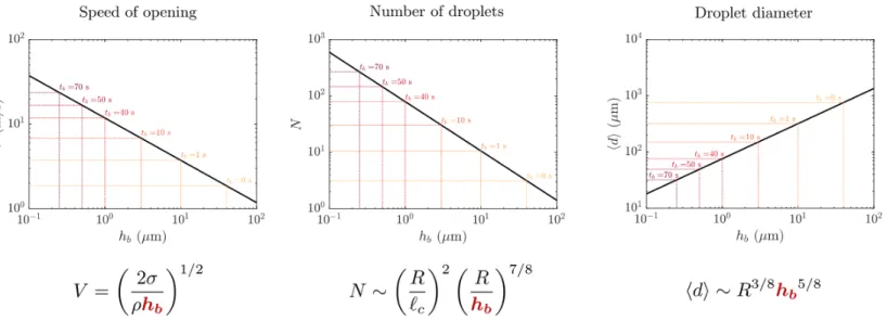
1-2 Influence of cap thickness for a given bubble radius, 𝑅, on 𝑉 the speed of the opening hole on the bubble, and the number 𝑁 and mean di-ameter ⟨𝑑⟩ of film droplets produced by the burst, where 𝜎 is surface tension of the bulk fluid, 𝜌 is density of the bulk fluid, ℎ𝑏is the thickness

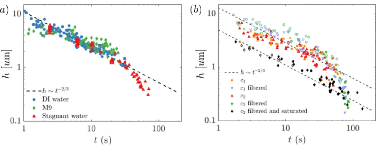
1-3 (𝑎) Thickness evolution of bubbles of radius 𝑅 = 5.5 ± 0.2 mm at ambient humidity for fresh deionized water, M9 medium diluted 20 times, and stagnant water. The diluted M9 culture medium does not significantly affect the lifetime nor thinning evolution of bubbles. (𝑏) Thickness evolution of bubbles with 𝑅 = 5.4 ± 0.2 mm derived from solutions of E.coli at 𝑐1 = 3 × 107 and 𝑐2 = 6 × 106 cells/mL, with or

without filtration of the bacteria. Solutions of filtered bacteria were obtained using a 0.22 𝑢m pore-size filter. The ambient humidity is 𝐻 = 22 ± 5%, and 𝐻 > 95% for saturated air conditions. All experiments in this study were conducted at ambient temperature 𝑇 = 24±1𝑜_𝐶. Filled

and open symbols show natural and manual bursts, respectively: due to their more deterministic lifetimes, bubbles from concentrated solutions of surfactants or bacterial secretions must be pierced manually with a needle to obtain their thickness at early times. Figures and data are from Poulain and Bourouiba [27]. . . 22

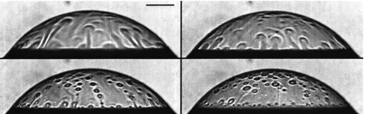
1-4 E.coli in a bubble film visualized using Schlieren imaging. The con-centration of bacteria is approximately 5 × 108 cells/mL in DI water.

The times are 𝑡 = 10s, 26s, 29s, and 36s. The corresponding bubble cap thickness are ℎ = 2.5𝑢m, 1.3𝑢m, 1.1𝑢m, and 0.9 𝑢m. Scale bar is 1mm. Reproduced from [28; 30] . . . 23

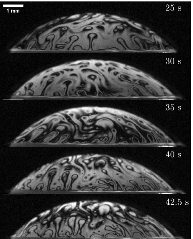
1-5 Temporal evolution of bubble cap composition shown by still-frame images of interferometry visualization for E.coli (𝐶𝐸.𝑐𝑜𝑙𝑖 = 1 × 107).

2-1 Diagram shows the path of light and the spacing of optical components in a Schlieren imaging setup based on Toepler’s dual-field-lens configu-ration [29]. Rays from an initial light source are collected and focused onto a pinhole to create a point source light, so that rays can be col-limated and passed through the objective area. In the objective area, light is deflected when it encounters changes in optical index, such as refractive changes through a soap film. The beam is refocused onto a camera sensor and differences are observed through interference patterns. 29 2-2 Thermal resistance circuit and model of the modified computer

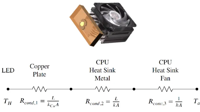
pro-cessing unit (CPU) heat sink for the light source. The CPU heat sink alone is rated for 100W, which is sufficient for three high-output LEDs operating at peak output. . . 30 2-3 Demonstration of vertical calibration procedure. (𝑎) shows the laser

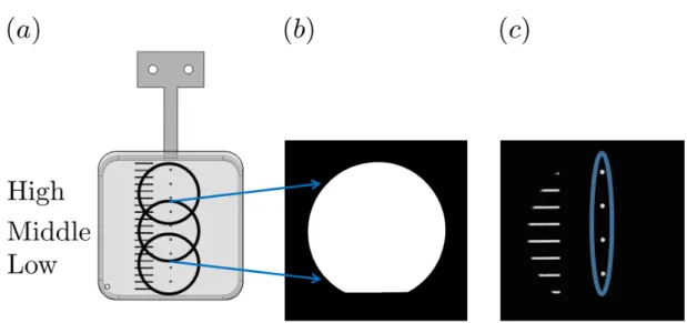
cut shutter frame that is placed over the film frame to enable vertical alignment of the system. Holes (𝑑 = 0.0635 cm) are cut at 10cm intervals from the base of the film frame. (𝑏) shows the unobstructed objective area and (𝑐) shows a representative image of the shutter plate placed over the film frame. This image is binarized and the coordinate location and the diameter of each circle is determined. Knowing this information allows us to define the relative position of every pixel in frame and set a representative length scale. . . 32 2-4 Surface tension of SDS solutions prepared in DI water at various

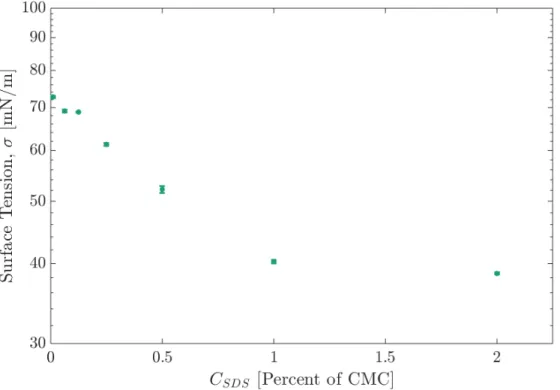
frac-tions of the Critical Micelle Concentration (CMC). These measure-ments are consistent with the literature [21]. . . 33 2-5 (𝑎) side and (𝑏) front view surface images of the 0.99 mm stainless

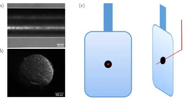
steel rod taken with a microscope. Scale bars are 250 𝑢m. (𝑐) shows the setup of the film frame apparatus. The rectangular frame is 3D printed with ABS plastic with the following dimensions 4” x 4” x 0.125”. The corners have a 0.5” radius to reduce sharp corners and prevent premature burst of the film. . . 34

3-1 Comparison of two concentrations of Nigrosin dye for light absorption method of measuring film thickness. We choose to use C = 2.4 gL−1

Nigrosin dye because it resulted in a lower standard deviation (𝜎1.2 =

19.60 [𝑢m]; 𝜎2.4 = 9.80[𝑢m]). . . 36

3-2 Comparison of the two approaches used to analyze film thickness data. Method 2 was much more successful in producing results in a reason-able range. . . 37 3-3 Thickness bands represent the average thickness measurement for all

pixels within a band spanning the width of the objective at the position of interest and of height of five pixels. . . 38 3-4 Visual representation of film thickness throughout the lifetime of a soap

film. This is data from a single trial where the middle region of the film frame is being observed. Scale bar is 20 mm. . . 39 3-5 Temporal evolution of film thickness at vertical positions within the

film. Each line represents the average of at least five trials, some include more because the placement of the objective area overlapped some positions (see Figure 2-3). Analysis begins at frame 200 (3.3 seconds) of each video to minimize the effect of plumes as the film forms and stabilizes. . . 40 3-6 Temporal evolution of film thickness at vertical positions within the

film. Each line represents the average of at least five trials, some include more because the placement of the objective area overlapped some positions (see Figure 2-3). Analysis begins at frame 200 (3.3 seconds) of each video to minimize the effect of plumes as the film forms and stabilizes. . . 41 3-7 Contact angle measurement. 𝜃1 and 𝜃2 are two contact angles measured

3-8 (𝑎) shows a representative frame from a spot size experiment using 0.99 mm stainless steel rod. This frame is taken at 𝑡 = 16.67 seconds. Local density gradients seen around spot create difficulties for image segmentation. (𝑏) demonstrates the steps taken to segment image in Matlab. Objective is to separate the spot from the background and disregard the vertical portion of the rod. (𝑐) masked image with fitted circle projected on the original image. (𝑑) Area of masked image and fitted circle plotted. Scale bar is 1 mm. . . 45 3-9 Schlieren spot size produced by rods of different materials. Each line

shows a time average of trials. Rod diameter (𝑑𝑟𝑜𝑑= 0.99 mm) and

vertical position (z = 50 cm) were held constant for all materials. . . 46 3-10 Schlieren spot size produced by rods with varying diameters. Each line

shows a time average of trials. Rod material (material: stainless steel) and vertical position (z = 50 cm) were held constant for all rod sizes. 47 3-11 Schlieren spot size produced by rods with varying diameters. Each line

shows a time average of trials. Rod material (material: stainless steel) and diameter (𝑑𝑟𝑜𝑑 = 0.99 mm) were held constant for all rod sizes. . 48

3-12 Schlieren spot size normalized by rod diameter and film thickness for each independent variable. Film thickness is calculated at each time step by interpolating experimental measurements of the temporal evo-lution of film thickness in Section 3.1. . . 49

List of Tables

3.1 Fluid properties (absortivity, 𝜖, and surface tension, 𝜎) and experimen-tal error for two different concentrations of Nigrosin die in solutions with DI water and the critical micelle concentration (CMC) of sodium dodecyl sulfate (SDS). . . 36 3.2 Summary of experimental parameters for rod in flat film experiments

with reference to figures. . . 43 3.3 Contact angles of the rods used in experiments. . . 44

Chapter 1

Introduction

1.1

Motivation

The dispersal of biological pathogens is a problem of interest due to its prevalence in healthcare (i.e. nosocomial infections), environmental phenomena (i.e. water-to-air dispersal from ocean spray), and intentional uses (i.e. mechanism of force or terrorism)[10; 32; 15; 5; 9; 38]. Much of our current understanding of surface bubbles was originally motivated by mysteries of public health. At the start of the 20th century, Major W. H. Horrocks conducted experiments to explore whether gas bubbles rising through sewage carried bacteria into the air, a common belief among sanitarians [25]. He conducted experiments to prove that bursting bubbles were a viable transfer mechanism to explain the link between the spread of bacteria from contaminated sewage to environmental air. Later, in 1948, when residents along the Florida Coast and Gulf of Mexico began to cough and experience a burning sensation in their eyes and respiratory tract, Woodcock was the first to trace the origin of the symptoms to an aerosol carried toxin. He hypothesized that this plankton-secreted toxin, which is now commonly referred to as Florida Red Tide, was transferred from the water to the air by bursting bubbles created by high winds and crashing waves in the surf [26]. Bursting bubbles play a central role in any scenario where pathogens are transferred between two immiscible fluids [10]. To obtain a comprehensive understanding of these processes, it is necessary to ensure that experimental techniques capture the

underlying mechanisms. The development of precise visualization techniques can provide insight into fluid contaminants and film physics at the interface.

Aerosols, which are microscopic particles (solid or liquid) suspended in a gas, are too small to be detected by the human eye and are often carried by the air that we breathe [2]. These particles, particularly bioaerosols like viruses, fungi, and bacteria, can be harmful in some situations due to either opportunistic pathogens like nosocomial infections (i.e. Clostridium Difficile spores spread from flushing toilets) or malicious intent in the release (i.e. antrax letters) [34; 26]. In his historical review of biological warfare, Riedel [41] cites instances of biological warfare conducted since 600BC. This strategy of attack was incredibly effective long before the science was understood due to the element of surprise and delayed effect. It turns out that bubbles and films are critical to understand to decipher how particles of contaminants disperse. Intrusions in thin films play a key role in shaping the final spray size and concentration.

1.2

The importance of film rupture

Bubbles are pervasive occurrences in nature, forming when interfaces between fluids are broken and air is mixed into the bulk [35]. They are the outcome of many natural processes like drop impact during rainfall [16; 36] and crashing surface waves in the ocean [5; 6], playing a critical role in natural ecosystems. Bubbles are a product of the environment in which they are formed. The interaction that bubbles have with the fluid bulk, which is rarely pure, influences the load of the secondary film and jet droplets that they will shed upon rupture. It is this subtle interplay between interfaces that links physics and biology [10].

Rupture of bubbles and films is a dominant mechanism in enabling transfer of a pathogen between fluids [10; 35]. As buoyant bubbles rise, they navigate through a fluid interacting with and scavenging particles suspended in their path [37; 6]. When bubbles and films rupture (discussed in further detail in Section 1.3), thousands of small droplets are transferred into the air. These have been “enriched,” having a much

Figure 1-1: Diagram of a surface bubble illustrating the concomitant effects of Marangoni stresses and curvature driven drainage described in the generalized drainage model proposed and validated in [28]. In this model of drainage, local temperature differences, which arise due to the relationship between water temper-ature 𝑇𝑤, temperature of the bubble cap 𝑇𝑐𝑎𝑝, and ambient air temperature 𝑇𝑎,

in-duce Marangoni stresses that either (𝑎) contribute to, or (𝑏) oppose curvature-driven drainage. (𝑐) Schematic shows “pinching” at the connection between the bulk fluid and the bubble cap (bubble foot) due to the balance between viscous stresses and capillary pressure. Figure from [28]. Other variables in diagram: H is relative humid-ity of the ambient air, ℎ is the bubble cap thickness, 𝑢∆𝑝 is the drainage velochumid-ity, and 𝑢∆𝜎 is the Marangoni flow

higher concentration that the bulk from which the bubble originated. Results in the literature vary depending on parameters like organism type, size, surface activity, and other physical properties, but the concentration in secondary droplets has been shown to range from 10-1000 times the concentration of the bulk [8; 7; 6].

1.3

An overview of bubble physics

Bubbles are gaseous volumes bound by an interface between a gas and a liquid, such as air and water. Molecules in a fluid system seek to minimize surface area and form spheres because surface tension makes the creation of a new surface energetically unfavorable [10; 18]. Surface tension, 𝜎 (𝑓 𝑜𝑟𝑐𝑒

𝑙𝑒𝑛𝑔𝑡ℎ or 𝑒𝑛𝑒𝑟𝑔𝑦

𝑎𝑟𝑒𝑎 ), is a measure of energy

loss per unit area that occurs at fluid interfaces. Bubbles are typically generated within the bulk via of mixing or degasing and they rise due buoyancy. When the bubble reaches the surface, it forms a water film, referred to as a bubble cap, which immediately begins to drain. The overpressure induced by curvature at the apex compared to the bulk water drives a flow from the cap towards the bulk: the bubble

Figure 1-2: Influence of cap thickness for a given bubble radius, 𝑅, on 𝑉 the speed of the opening hole on the bubble, and the number 𝑁 and mean diameter ⟨𝑑⟩ of film droplets produced by the burst, where 𝜎 is surface tension of the bulk fluid, 𝜌 is density of the bulk fluid, ℎ𝑏 is the thickness of the bubble at burst, 𝑙𝑐 = √︀𝜎/𝜌𝑔 is

the capillary length, [18; 28].

cap drains. [18] derived the expression of the thickness evolution of this film as (shown in the form presented by Poulain et al. [28]):

ℎ(𝑡) ∼ 𝑙𝑐 (︂ 𝑡𝑣 𝑡 )︂2/3_{(︂ 𝑅} 𝑙𝑐 )︂7/3 with 𝑡𝑣 = 𝜇𝑙𝑐 𝜎 and 𝑙𝑐= √︀ 𝜎/𝜌𝑔 (1.1) This expression shows that the time dependence of the bubble cap thickness has the following scaling:

ℎ(𝑡) ∼ 𝑡−2/3 (1.2) The predicted scaling law ℎ ∼ 𝑡−2/3 _{has been validated with various water sources}

(i.e. deionized (DI) water, Massachusetts Charles River, and tap water from various locations) at ambient temperature and without evaporation [18; 28]. Temperature and air saturation do not significantly affect the time dependence of the cap thinning at short times, but they do influence the magnitude of the cap thickness. Marangoni stresses that arise from local temperature gradients drive a flow that either contributes to or counteracts curvature-driven drainage (illustrated in Figure 1-1).

Using the Taylor-Culick velocity of the receding hole on the cap of a bursting bubble, the bubble cap thickness at the time of burst can be indirectly measured using Equation 1.3.

ℎ𝑏 =

2𝜎

𝜌𝑉2 (1.3)

Experimental validation of the temporal evolution of bubble cap drainage is es-sential to understanding how bursting bubbles transfer aerosols from a bulk fluid to their environment. Taylor-Culick velocity (𝑉 ), number of secondary droplets pro-duced by a bubble burst (𝑁), and mean droplet diameter (⟨𝑑⟩) all scale with bubble cap thickness as shown in Figure 1-2 [18; 28]. Since bubbles thin as they age due to the drainage that occurs continuously from when bubbles reach an air-water interface, the cap of older bubbles ruptures with a higher opening velocity, and thus produces more secondary droplets with smaller mean diameters. This effect of extended bubble lifetime can significantly enhance the aerosolization of the bulk solution’s load into its environment [28; 27].

1.4

Altered physics of bubbles at contaminated

in-terfaces

Section 1.3 describes how bubble cap thickness evolves for “clean” solutions, but here we will discuss how thinning changes for “dirty” bubbles. Poulain and Bourouiba [27] study bubbles in solutions containing Escherichia coli (E.coli) and show that bacterial secretions in the solutions extend the lifetime of bubbles. The ℎ ∼ 𝑡−2/3 _{scaling law}

from the classic drainage model still applies, but only until a critical transition time 𝑡𝑐 and thickness to an evaporation-dominated regime occurs. Thinning occurs at a

higher rate in this evaporation regime compared to the 𝑡−2/3 _{drainage for those low}

thicknesses, which manifests as a “kink” on plots of the thickness evolution (see Figure 1-3). In accordance with the scaling estimated by [18], the bubbles that burst in this regime will produce smaller and more droplets than bursts of the average clean bubble

Figure 1-3: (𝑎) Thickness evolution of bubbles of radius 𝑅 = 5.5±0.2 mm at ambient humidity for fresh deionized water, M9 medium diluted 20 times, and stagnant water. The diluted M9 culture medium does not significantly affect the lifetime nor thinning evolution of bubbles. (𝑏) Thickness evolution of bubbles with 𝑅 = 5.4 ± 0.2 mm derived from solutions of E.coli at 𝑐1 = 3 × 107 and 𝑐2 = 6 × 106 cells/mL, with or

without filtration of the bacteria. Solutions of filtered bacteria were obtained using a 0.22 𝑢m pore-size filter. The ambient humidity is 𝐻 = 22 ± 5%, and 𝐻 > 95% for saturated air conditions. All experiments in this study were conducted at ambient temperature 𝑇 = 24±1𝑜_{𝐶. Filled and open symbols show natural and manual bursts,}

respectively: due to their more deterministic lifetimes, bubbles from concentrated solutions of surfactants or bacterial secretions must be pierced manually with a needle to obtain their thickness at early times. Figures and data are from Poulain and Bourouiba [27].

at the same lifetime. The size and quantity of the droplets produced in this regime make it more likely that the droplets will remain suspended in the air and spread the pathogen. This information is critical to understanding the mechanism of pathogen transfer from a bulk fluid to its surrounding environment because it explains one way microorganisms can manipulate the physics of bubble cap thinning to enhance pathogen dispersal.

Studies validated the impact of this mechanism of transfer, showing that the secondary film droplets produced from a bubble burst can have 10-1000x higher concentrations than the bulk solution from which they originated. This phenom-ena of enrichment proposes a very intriguing research problem, because although it is reported in the literature there is not a consensus regarding the mechanisms of

Figure 1-4: E.coli in a bubble film visualized using Schlieren imaging. The concentra-tion of bacteria is approximately 5×108 _{cells/mL in DI water. The times are 𝑡 = 10s,}

26s, 29s, and 36s. The corresponding bubble cap thickness are ℎ = 2.5𝑢m, 1.3𝑢m, 1.1𝑢m, and 0.9 𝑢m. Scale bar is 1mm. Reproduced from [28; 30]

enrichment [7; 6]. Poulain and Bourouiba [27] observed bacteria on bubbles in con-taminated solutions with interferometry imaging (shown in Figure 1-5) and Schlieren imaging [28; 30] shown in Figure 1-4. The content at the cap was explained by Su and Bourouiba [30]. However, a number of questions remain open to understand film deformation and stability when subjected to intrusions.

1.5

Flat soap films

For this study, we intend to use flat, vertical films as a simplified analog for sur-face bubbles. A soap film can be thought of as water molecules layered between two soap monolayers with a thickness on the order of 10-100 microns [14; 11]. Generally, drainage is dominated by gravity which induces a thickness gradient from top to bot-tom of the film. Interference creates selective reflection at certain optical wavelengths that is characteristic of the film thickness. Once parts of the film thin to the point where only a few water molecules remain sandwiched inbetween the two monolayers of soap no more optical interference effects can be seen and the film appears “black.” Mysels [23; 11] classifies soap films with the following terms:

1. Generation

Figure 1-5: Temporal evolution of bubble cap composition shown by still-frame images of interferometry visualization for E.coli (𝐶𝐸.𝑐𝑜𝑙𝑖 = 1 × 107). Experiments reproduced

• Pull-out: a moving frame pulling fluid out of a reservoir 2. Drainage

• Rigid: surfactants covering the films are either highly viscous or in solid-phase, so drainage primarily takes place as Poisseuille flow between the surfactant layers

• Mobile: low viscosity surfactant molecules cover the film surface so drainage takes place as a two dimensional flow of the combined surfactant-water sys-tem

For our experiments, we easily form “mobile, pull-out” soap films by pulling a plastic frame from a tank filled with surfactant solution. Although soap films have been a topic of scientific fascination since Newton’s investigation of “black films,” many of the deterministic properties and interactions of the films remained questions for a long time. Experimentally derived profiles of film thickness were measured directly using methods like reflectometry [20], interferometry [1; 22], and schlieren imaging [4; 3], or measured indirectly using the Taylor-Culick relation to measure the velocity of the hole expansion of ruptured films [31; 12; 18; 24]. The basis of our theoretical understanding of vertical film thickness comes from Frankel’s Law, which models both film interfaces as rigid bodies that influence the initial thickness, ℎ0,

through shear-like dynamics [23]: ℎ0 𝑙𝑐 = 1.89(︂ 𝜂𝑈 𝜎 )︂2/3 = 1.89 𝐶_𝑎(2/3), (1.4) where 𝑙𝑐=√︀𝜎/𝜌𝑔is the capillary length, 𝜂 is the viscosity of the fluid, 𝑈 is the speed

at which the film is pulled out of the solution, 𝛾 is the surface tension, and 𝐶𝑎 is the

capillary number. It is worth noting that Frankel’s Law has been challenged on the fact that the film dynamics are likely modelled more accurately as extensional flow that is dominated by surface viscous stresses, but this does not affect the power law, it only adjusts the pre-factor [33].

De Gennes [13] proposed the following one-dimensional film thickness profile based on the distribution of surfactants within the film:

ℎ0 =

2Γ𝐵

𝑐𝐵− 𝑐

(1.5)

where Γ𝐵 is the bulk surfactant monolayer concentration, 𝑐𝐵 is the bulk concentration

Chapter 2

Experimental setup and methods

The experiments conducted by Poulain and Bourouiba [27] (described in detail in Section 1.4) captured the appearance of spots on the bubble caps in contaminated solutions. Quantifying data was extracted in Su and Bourouiba [30]. However, a num-ber of open questions remain. Here, we revisit these questions with a soap film with higher concentration of surfactant to explore if the film deformation is affected. We make qualitative inferences about the appearance of particles on the bubble cap. The experiments described in this paper aim to investigate the factors that influence the apparent size of particles in thin films laden with surfactants at CMC concentration. With the method proposed here, we quantify concentration and assess size of objects, which can enable characterization of interaction, assembly, and repulsion between particles or organisms and do so over a large scale when films are stabilized by surfactants. Eventually, this capability could reveal patterns of assembly and interactions that would go otherwise unseen and give insights into film deformation and stability.

2.1

Optical principals of Schlieren imaging

Similar to Poulain and Bourouiba [27] and Su and Bourouiba [30], we use Schlieren imaging to visualize local density gradients caused by deformation of the thin film around objects and small particles. Light propagates uniformly through homogeneous

media, but when light travels through regions of nonuniform density the rays of light bend. Schlieren visualization capitalizes on this effect to reveal density variations [29; 31]. The refractive index, 𝑛 = 𝑐0

𝑐, represents the interaction between light and

matter by comparing the speed of light in the medium, 𝑐, to the speed of light in a vacuum, 𝑐0. In air and other gases, the index of refection has a weak linear

dependence on medium density, which for ideal gases is linearly related to temperature and pressure of the medium. With the right optical equipment, properly constructed and aligned, we can visualize small variations in temperature, pressure, and density. In fact, Toepler showed in the 19𝑡ℎ _{century that this technique is sensitive enough to}

optically detect a 1°C temperature difference, which is equivalent to a one part per million change in index of refraction [29].

We set up a Schlieren system in accordance with the configuration of Toepler’s dual-field-lens arrangement using a point source light, a pinhole, four lenses, and a camera. A diagram of the lens arrangement is shown in Figure 2-1, as well as images of the convection plumes from a small candle and from human speech to serve as intuitive functional examples. In order to gain insight into what is observed with bacteria on bubbles, we use objects (rods and microparticles) of known sizes to develop a calibration relating the size of the Schlieren spot to the actual size of the object. Objects within thin films create black spots in Schlieren images due to the local thickness gradient formed by the film around the intrusion (i.e. particles and microbubbles in [28]). Additionally, we choose to use vertical soap films to limit the complexity of geometry and eliminate the competing effect of drainage and regeneration [28]. With flat films, we are also able to guarantee that rods always penetrate the film normal to its surface. Our experimental results are compared to ray-tracing and numerical simulation results conducted by Su and Bourouiba [30] which show the theoretical spot size based on the experimental setup and physical properties of the obtrusion by factoring in the meniscus profile described in Section 1.5.

Center of Curvature LED

1

Aspheric Condenser Lenses

2

Pinhole

3 4

Achromatic Field Lenses

Objective Area

Rectangular Aperture and Camera

𝑓

𝑓

𝑓

𝑓3

+ 𝑓

𝑓

Figure 2-1: Diagram shows the path of light and the spacing of optical components in a Schlieren imaging setup based on Toepler’s dual-field-lens configuration [29]. Rays from an initial light source are collected and focused onto a pinhole to create a point source light, so that rays can be collimated and passed through the objective area. In the objective area, light is deflected when it encounters changes in optical index, such as refractive changes through a soap film. The beam is refocused onto a camera sensor and differences are observed through interference patterns.

2.2

Novel design for thin film generation and

obser-vation

The experimental apparatus is designed to allow for communication between com-partments of the system for complete automation, streamlined data collection, and precise control over parameters that affect thin film dynamics. A break in the optical rail that houses the lenses allows the user to easily exchange the objective (i.e. verti-cal film frame, bubble generating tube, acoustic levitation field) without altering the optical alignment. The optical elements are fixed to rails on both sides of the objec-tive area, the first of which is fixed to the optical table and the second is attached to an adjustment apparatus that allows the rail to rotate. This feature allows the user micron-precision adjustment to ensure perfect alignment of the optical elements on both sides of the objective area. The objective area is completely enclosed in a 12” x 12” x 18” housing that is sealed to control temperature and relative humidity, and to protect the objective from external airflow that could induce perturbation and premature burst [14]. The housing has optical windows in-line with the optical elements so that the light does not have to travel through two additional mediums and potentially skew the Schlieren image.

Figure 2-2: Thermal resistance circuit and model of the modified computer processing unit (CPU) heat sink for the light source. The CPU heat sink alone is rated for 100W, which is sufficient for three high-output LEDs operating at peak output.

A high luminance light source with approximate spacial coherence is a key re-quirement for sharp Schlieren images [29]. In order to fulfill this rere-quirement, we use a point-source Light-Emitting Diode (LED) that produces 32W power and 4022 lu-minous flux at peak output. A CPU heat sink was outfitting for the setup so that the light source could operate at peak output for extended periods without modulation of the light intensity. Figure 2-2 shows a thermal circuit schematic of the heat sink, illustrating that it meets the performance requirements for consistent operation of the LED, which is extremely important for image processing of videos, particularly those that compare frame intensity to background intensity. This light is gathered and focused onto a pinhole by a pair of aspheric condenser lenses in order to replicate a true point source light. This light is collimated by the first of a set of field lenses and then refocused onto the cutoff plane of a rectangular aperture.

The apparatus used for film formation was based on the method described by Mcentee et al. [20]. In contrast to their method, we form the film by lowering the

solution tank, a 6” x 6” x 1.5” acrylic chamber filled with surfactant solution, rather than moving the soap film frame. This method keeps the film frame fixed and re-duces the impact of any mechanical vibrations. The stage, driven by means of an electronically controlled stepper motor at approximately 7.5 cm/s, moves the solu-tion tank from engulfing the soap film frame to completely below it. Coordinasolu-tion of film formation ensues automatically after the user initiates an experimental trial:

1. Heat sink fan turns off.

2. Light source turns on.

3. Temperature and relative humidity are recorded.

4. High speed camera recording initiated.

5. Solution table moves to down position.

6. User signals end of trial. Setup moves back to OFF position with solution tank in up position, heat sink fan on to cool LED, light source off, and camera ready to record.

The optical elements that we use to construct this setup have a two inch diameter, so at a single position we are only able to view and record a portion of the soap film. Since the vertical position of the optical element is fixed, we adjust the position of the film frame in order to collect data over the full vertical range of the film. Knowing the vertical position of the objective is important because film thickness varies vertically due to gravity-driven drainage [30]. We use a laser-cut shutter plate to ensure vertical alignment of the system, allowing us to define pixel coordinates relative to the bottom of the film frame. Figure 2-3 further explains this process.

Figure 2-3: Demonstration of vertical calibration procedure. (𝑎) shows the laser cut shutter frame that is placed over the film frame to enable vertical alignment of the system. Holes (𝑑 = 0.0635 cm) are cut at 10cm intervals from the base of the film frame. (𝑏) shows the unobstructed objective area and (𝑐) shows a representative image of the shutter plate placed over the film frame. This image is binarized and the coordinate location and the diameter of each circle is determined. Knowing this information allows us to define the relative position of every pixel in frame and set a representative length scale.

Figure 2-4: Surface tension of SDS solutions prepared in DI water at various fractions of the Critical Micelle Concentration (CMC). These measurements are consistent with the literature [21].

2.3

Experimental procedure

2.3.1

Preparation of surfactant solution

Sodium dodecyl sulfate (SDS) was chosen as the non-organic surfactant because it has been shown to have less effect on the Marangoni flow and bubble bursting dynamics than other surfactants, specifically Tween and 𝐶14TAB [28; 27]. Figure 2-4) shows a

characterization of the surface tension of SDS at different concentrations in DI water solutions. Here we use a surfactant concentration of 100% of the Critical Micelle Concentration (CMC) of SDS for experiments to ensure that the films were able to sustain themselves with rod intrusions. This is in contrast to results discussed in [30] where lower surfactant concentrations were used. Large batches of SDS were mixed and stored at room temperature and isolated from light to prevent degradation of the aqueous solutions [19]. Each batch was used for experimental trials for up to a week.

Figure 2-5: (𝑎) side and (𝑏) front view surface images of the 0.99 mm stainless steel rod taken with a microscope. Scale bars are 250 𝑢m. (𝑐) shows the setup of the film frame apparatus. The rectangular frame is 3D printed with ABS plastic with the following dimensions 4” x 4” x 0.125”. The corners have a 0.5” radius to reduce sharp corners and prevent premature burst of the film.

2.3.2

Preparation of rods for experiments

Each rod was bent precisely to 90𝑜 _{to ensure that it is normal to the plane of the}

soap film when protruding through and limits obstruction of the system’s lighting. Softer metals, like copper and nickel that only come wound in spools, have to be straightened first. This is done by holding the wire with a vice grip and applying a tension force. The rods are then bent to 90𝑜 _{with a bending brake machine.}

Chapter 3

Results

The shape of the meniscus formed around a spherical particle, reviewed thoroughly in Section 1.5, is determined by film thickness, particle radius, and particle wetting properties. We conduct a series of experiments in attempt to isolate the effect of each variable and determine a relationship between them.

3.1

Measuring film thickness

Understanding how film thickness varies with time and vertical position is an essential piece to understanding the evolution of Schlieren spots observed in thin films. We mix Nigrosin dye with the solution of SDS and DI water to measure the film thickness using the light adsorption method [36; 34; 17]. This method operates on the principal that the portion of light adsorbed as it passes through a thin film of dyed liquid is proportional to the thickness of the film. We use the experimental calibration from Wang and Bourouiba [36] to define the fluid absorptivity of the dye solution, which gives the relationship between intensity and film thickness according to the Beer-Lambert law of absorption:

Concentration Surface tension, 𝜎 Absorptivity, 𝜖 Standard deviation, 𝜎 of film thickness 1.2 [gL−1_{] 41.6 [mN/m] 185.1 [𝑢m] 19.60 [𝑢m]}

2.4 [gL−1_{] 47.1 [mN/m] 92.55 [𝑢m] 9.80 [𝑢m]}

Table 3.1: Fluid properties (absortivity, 𝜖, and surface tension, 𝜎) and experimental error for two different concentrations of Nigrosin die in solutions with DI water and the critical micelle concentration (CMC) of sodium dodecyl sulfate (SDS).

Figure 3-1: Comparison of two concentrations of Nigrosin dye for light absorption method of measuring film thickness. We choose to use C = 2.4 gL−1 _{Nigrosin dye}

because it resulted in a lower standard deviation (𝜎1.2 = 19.60[𝑢m]; 𝜎2.4 = 9.80[𝑢m]).

Eventually, we decided to use a higher concentration of Nigrosin dye after finding that the solution with the higher concentration of dye had a lower standard deviation between trials than the lower concentration solution (see Figure 3-1). The higher concentration allows for higher resolution given that the magnitude of film thickness measurements is smaller than what was studied in the previous application (ℎ > 40𝑢m). Based on a meticulous calibration conducted for their study, the value for the fluid absorptivity, 𝜖, was easily adjusted for the concentration that we chose (Table 3.1).

Figure 3-2: Comparison of the two approaches used to analyze film thickness data. Method 2 was much more successful in producing results in a reasonable range.

sensitive to changes in experimental conditions and changes in background lighting. Care was taken to limit contributions from other light sources in the laboratory, to ensure consistent power settings, and to design a sufficient heat sink to limit fluctuations of the light source caused by thermal resistance (see Figure 2-2). The first attempt at processing this data produced skewed results because of image processing mishaps. The first method assumes constant background intensity, 𝐼0, and uses a

single image for the background intensity values for all trails. The second method uses the final frame from each trial, which was saved so the last frame was post-burst of the film, for the background intensity values for that trial. Additionally, the first method normalized pixel values for each frame of the video before comparing to the background intensity. This step increased the image contrast and made the image easier to qualitatively analyze, but it also skewed calculation for film thickness. Results from the same data set, processed using both methods, are shown in Figure 3-2.

Figure 3-6 shows the temporal evolution of film thickness at ten centimeter in-tervals within the film frame. We refer to each vertical position as a “band” because

Figure 3-3: Thickness bands represent the average thickness measurement for all pixels within a band spanning the width of the objective at the position of interest and of height of five pixels.

they are the average values from a block of pixels surrounding the objective positions. This grouping is further illustrated in Figure 3-3.

In order to capture the full spectrum of vertical positions, the film frame was positioned at three different heights (demonstrated in Figure 2-3) and the data was overlayed in post-processing. Figure 3-5 shows the raw data for each trial conducted sorted by vertical position. Data is not reported prior to frame 200 (𝑡 = 3.33 seconds) while the film is forming and stabilizing. The exact positioning of the film frame is not important because the low, middle, high positions covered the span of the film frame.

The time average of the film thickness data is aggregated and reported in Figure 3-6. The averaged data only takes into account the first 20 seconds of the film’s existence and neglects films that burst prior to this threshold. It is intuitive and clear that a thickness gradient is maintained from the top of the frame to the bottom. The relatively consistent difference in thickness from the top band (𝑧 = 80 cm) to the bottom band (𝑧 = 10 cm) infers that the draining fluid pools below the bottom band of measurement, possibly on the rim of the film frame. The film continues to drain after it reaches equilibrium in the early seconds of its life, but at a much slower rate.

Figure 3-4: Visual representation of film thickness throughout the lifetime of a soap film. This is data from a single trial where the middle region of the film frame is being observed. Scale bar is 20 mm.

Solution: DI water + 1CMC SDS + 2.4 g/L Nigrosin dye Lighting: 6.3V input to CREE LED array

Figure 3-5: Temporal evolution of film thickness at vertical positions within the film. Each line represents the average of at least five trials, some include more because the placement of the objective area overlapped some positions (see Figure 2-3). Analysis begins at frame 200 (3.3 seconds) of each video to minimize the effect of plumes as the film forms and stabilizes.

Figure 3-6: Temporal evolution of film thickness at vertical positions within the film. Each line represents the average of at least five trials, some include more because the placement of the objective area overlapped some positions (see Figure 2-3). Analysis begins at frame 200 (3.3 seconds) of each video to minimize the effect of plumes as the film forms and stabilizes.

3.2

Schlieren visualization

3.2.1

Rods in flat films

We see that bacteria are revealed macroscopically on bubbles when the cap film becomes thin enough [28; 30]. Here we revisit the imaging for higher surfactant concentrations. Using rods to penetrate the soap film enables more control to isolate the variables that effect the Schlieren spot size. Rods can be fixed in position and come with commercially available options that allow the variance of size and material properties. Piercing the film with objects that are 50 to 100 times greater than the thickness of the film justify an important simplifying assumption to neglect the influence of film thickness.

Our experimental setup is presented in Section 2.2. In this paper, we study the effect of three variables on spot size:

1. Rod material (stainless steel, aluminum, copper, nickel)

2. Rod diameter (𝐷𝑟𝑜𝑑 =0.99 mm, 0.74 mm, 0.51 mm, 0.38 mm, 0.25 mm)

3. Rod position (z = 10 cm, 50 cm, 80 cm)

Table 3.2 shows a summary of experiments conducted.

We measured the contact angle of each rod by dipping them in a reservoir of solution with the same composition as the one used to conduct experiments (see Figure 3-7). There was minimal variation in contact angle among materials, ranging from 25𝑜 to 45𝑜 for all rods studied (results presented in Table 3.3). We then compare

our experimental data with the Schlieren simulations conducted in Su and Bourouiba [30].

Objective Rod material Rod diameter Rod position Results Material Stainless steel 0.99 mm Middle (z = 50 cm) Figure 3-9

Aluminum Copper

Nickel

Diameter Stainless steel 0.99 mm Middle (z = 50 cm) Figure 3-10 0.74 mm

0.51 mm 0.38 mm 0.25 mm

Position Stainless steel 0.99 mm Low (z = 10 cm) Figure 3-11 Middle (z = 50 cm)

High (z = 80 cm)

Table 3.2: Summary of experimental parameters for rod in flat film experiments with reference to figures.

Material Contact angle Stainless steel 35𝑜

Aluminum 41𝑜

Copper 45𝑜

Nickel 25𝑜

Table 3.3: Contact angles of the rods used in experiments.

Figure 3-7: Contact angle measurement. 𝜃1 and 𝜃2 are two contact angles measured

manually using ImageJ.

3.2.2

Image processing of spot size videos

Figure 3-8 shows a representative frame from an experimental trial and different steps in the process to segment the image so that the Schlieren spot is distinct from the background. This image processing proved to be difficult because the background of the image constantly fluctuated as film drained around the cylindrical intrusion.

Figure 3-8: (𝑎) shows a representative frame from a spot size experiment using 0.99 mm stainless steel rod. This frame is taken at 𝑡 = 16.67 seconds. Local density gra-dients seen around spot create difficulties for image segmentation. (𝑏) demonstrates the steps taken to segment image in Matlab. Objective is to separate the spot from the background and disregard the vertical portion of the rod. (𝑐) masked image with fitted circle projected on the original image. (𝑑) Area of masked image and fitted circle plotted. Scale bar is 1 mm.

3.2.3

Effect of rod material

Experimental results are presented in Figure 3-9 for this round of tests. The rod diameter and vertical position were held constant, so that only the rod material was changed between trials to isolate the effect of material properties. Variations for different materials, and hence different contact angles, are small. These results show that wetting properties do not seem to have a dominant effect on the size of the Schlieren spot in the limit where the obtrusion is much larger than the thickness of the film. This finding is in agreement results from Su and Bourouiba [30] (for water films) that show wetting properties do not play a significant role when the intrusion is much larger than the film (larger than 150 𝑢m).

Figure 3-9: Schlieren spot size produced by rods of different materials. Each line shows a time average of trials. Rod diameter (𝑑𝑟𝑜𝑑= 0.99 mm) and vertical position

3.2.4

Effect of rod diameter

Here, we investigate the effect of rod diameter on the size of the Schlieren spot observed. Our experimental results are represented in Figure 3-10. In this round of tests, the rod material and vertical position were constant, so that only the rod diameter was changed between trials to isolate the effect of obtrusion size. Variations for different sizes are present and similar to the difference of the rod diameter.

Figure 3-10: Schlieren spot size produced by rods with varying diameters. Each line shows a time average of trials. Rod material (material: stainless steel) and vertical position (z = 50 cm) were held constant for all rod sizes.

3.2.5

Effect of rod position

Now, we investigate the effect of rod position on the size of the Schlieren spot observed. Our experimental results are represented in Figure 3-11. In this round of tests, the rod material and diameter were constant, so that only the vertical position of the rod

was changed between trials to isolate the effect of film thickness.

Figure 3-11: Schlieren spot size produced by rods with varying diameters. Each line shows a time average of trials. Rod material (material: stainless steel) and diameter (𝑑𝑟𝑜𝑑 = 0.99 mm) were held constant for all rod sizes.

3.2.6

Summary of spot size results with rods

Figure 3-12 shows the normalized spot size for the investigation of each independent variable:

𝑑𝑛𝑜𝑟𝑚𝑎𝑙𝑖𝑧𝑒𝑑 =

𝑑𝑠𝑝𝑜𝑡− 𝑑𝑟𝑜𝑑

Figure 3-12: Schlieren spot size normalized by rod diameter and film thickness for each independent variable. Film thickness is calculated at each time step by interpolating experimental measurements of the temporal evolution of film thickness in Section 3.1.

Chapter 4

Discussion and conclusion

As we’ve discussed, rupturing films and bubbles are a prevalent mechanism of trans-ferring particles from a fluid into the atmosphere. The mechanisms of transfer have been a question of scientific intrigue for many years now. It started with anecdotal observations of bacterial infection arriving from puzzling sources, the underground sewer or the coast that was miles away. These occurrences pushed scientists to inves-tigate the root cause. Not only did they find that bubbles were an efficient method of moving organisms across interfaces, but that it seemed to be an extremely efficient means of doing so. In the mid-twentieth century, the body of knowledge was further elucidated by the efforts of G.I. Taylor and Fred Culick as they theoretically and experimentally (with the advent of Doc. Edgerton’s high speed imaging) revealed the violence of film rupture. Although we have made significant progress in understanding the complex dynamics that govern bubble and film dynamics, many questions remain unanswered. We still don’t understand the dominant mechanisms of film deformation and rupture from intrusions. In order to reveal this information, we must have the means to systematically and precisely observe particle interactions within a film in real-time at a macroscopic scale.

In this study, we developed a method that can inform the direct observation of contaminants interacting with a soap film in which the intrusions are trapped. In the first part of the study, we develop an apparatus to directly observe microscale interactions within films. This novel design allows us to systematically study an

objective of our choosing. Here, we choose to investigate which properties affect the size of the optical spot created by intrusions in soap films as a function of film thickness and wetting. The experimental design is careful to account for parameters that could confound results by ensuring consistent environmental parameters, precise positioning of the object, and accounting for thickness of the film over time. We use high levels of pure surfactant to generate films that can sustain themselves despite being punctured by large objects (𝑑𝑟𝑜𝑑 >> ℎ𝑓 𝑖𝑙𝑚).

Using this approach, we are able to validate and extend the results found by Su and Bourouiba [30] by showing that the Schlieren spot size produced by large objects is not affected by size or wetting properties of the object. The spot size is affected by film thickness, and the plumes resulting from Marangoni flows on soap films. In following experiments, we could also vary the same properties that we did here but on the microscale. This will allow us to fully classify the appearance and interaction of different types of organisms and work towards a calibration between what we observe with this imaging technique and what is truly present in soap films or surfactant-laden films in general.

In summary, the project focused on the development and refinement of a novel technique to study distortion of elastic interfaces and its optical measurement. These experiments focused on providing insight into what is observed within films with intrusions that were much larger than the film thickness.

Bibliography

[1] Y. D. Afanasyev, G. T. Andrews, and C. G. Deacon. Measuring soap bubble thickness with color matching. American Journal of Physics, 79(10):1079–1082, 2011. ISSN 0002-9505. doi: 10.1119/1.3596431.

[2] M. Alsved, L. Bourouiba, C. Duchaine, J. Löndahl, L. C. Marr, S. T. Parker, A. J. Prussin, and R. J. Thomas. Natural sources and experimental generation of bioaerosols: Challenges and perspectives. Aerosol Science and Technology, 0(0):1–25, 2019. ISSN 15217388. doi: 10.1080/02786826.2019.1682509. URL https://doi.org/10.1080/02786826.2019.1682509.

[3] B. Atcheson. Schlieren-Based Flow Imaging. 2004.

[4] M. I. Auliel, F. Castro Hebrero, R. Sosa, and G. Artana. Schlieren technique in soap film flows. 58:38, 2017. doi: 10.1007/s00348-017-2311-4.

[5] E. R. Baylor, V. Peters, and M. B. Baylor. Water-to-air transfer of virus. Science, 197(4305):763–764, 1977. ISSN 00368075. doi: 10.1126/science.329413.

[6] D. C. Blanchard. The Ejection of Drops from the Sea and Their Enrichment with Bacteria and Other Materials: A Review. Estuaries, 12(3):127–137, 1989. ISSN 01608347. doi: 10.2307/1351816. URL http://link.springer.com/10. 2307/1351816.

[7] D. C. Blanchard and L. Syzdek. Mechanism for the water-to-air transfer and concentration of bacteria. Science, 170(3958):626–628, 1970. ISSN 00368075. doi: 10.1126/science.170.3958.626.

[8] D. C. Blanchard and L. D. Syzdek. Bubble tube: Apparatus for determining rate of collection of bacteria by an air bubble rising in water. Limnology and Oceanography, 19(1):133–138, 1974. ISSN 19395590. doi: 10.4319/lo.1974.19.1. 0133.

[9] D. C. Blanchard and L. D. Syzdek. Water-to-air transfer and enrichment of bac-teria in drops from bursting bubbles. Applied and Environmental Microbiology, 43(5):1001–1005, 1982. ISSN 00992240.

[10] L. Bourouiba and J. W. Bush. Drops and bubbles in the environment. Handbook of Environmental Fluid Dynamics, Volume One: Overview and Fundamentals, pages 427–439, 2012. doi: 10.1201/b14241.

[11] R. Bruinsma. Theory of hydrodynamic convection in soap films. Physica A, 216: 59–76, 1995.

[12] F. E. C. Culick. Comments on a Ruptured Soap Film. Journal of Applied Physics, 31:1128–1129, 1960. doi: 10.1063/1.1735765. URL https://doi.org/10.1063/ 1.1735765.

[13] P. G. De Gennes. "Young" soap films. Langmuir, 17(8):2416–2419, 2001. ISSN 07437463. doi: 10.1021/la001538l.

[14] P.-G. de Gennes, F. Brochard-Wyart, and D. Quere. Capillarity and Wetting Phenomena. Springer Science and Business Media LLC, New York, 2003. [15] A. G. Garza, S. M. Van Cuyk, M. J. Brown, and K. M. Omberg. Detection of

the Urban Release of a Bacillus anthracis Simulant by Air Sampling . Biosecurity and Bioterrorism: Biodefense Strategy, Practice, and Science, 12(2):66–75, 2014. ISSN 1538-7135. doi: 10.1089/bsp.2013.0086.

[16] C. Josserand and S. Thoroddsen. Drop Impact on a Solid Surface. Annual Review of Fluid Mechanics, 48(1):365–391, 2016. ISSN 0066-4189. doi: 10.1146/ annurev-fluid-122414-034401. URL http://www.annualreviews.org/doi/10. 1146/annurev-fluid-122414-034401.

[17] J. Kim and M. H. Kim. A Photochromic Dye Activation Method for Measuring the Thickness of Liquid Films. Bull. Korean Chemical Society, 26(6):966–970, 2005.

[18] H. Lhuissier and E. Villermaux. Bursting bubble aerosols. Journal of Fluid Mechanics, 696:5–44, 2012. ISSN 00221120. doi: 10.1017/jfm.2011.418.

[19] K. Lunkenheimer and G. Czichocki. On the Stability of Aqueous Sodium Dodecyl Sulfate Solutions. Journal of Colloid and Interface Science, 160:509–510, 1993. [20] W. R. Mcentee, W. R. Mcentee, and K. J. Mysels. The Bursting of Soap Films.

I. An Experimental Study. The Journal of Physical Chemistry, 73(9):3018–3028, 1969. doi: 10.1021/j100843a042.

[21] K. J. Mysels. Surface Tension of Solutions of Pure Sodium Dodecyl Sulfate. Langmuir, 2(4):423–428, 1986. doi: 10.1021/la00070a008.

[22] K. J. Mysels and M. C. Cox. An experimental test of Frankel’s Law of film thickness. Journal of Colloid Science, 17(2):136–145, 1962. ISSN 00958522. doi: 10.1016/0095-8522(62)90004-1.

[23] K. J. Mysels, K. Shinoda, and S. Frankel. Soap films: studies of their thinning and a bibliography. 1959.

[24] A. B. Pandit and J. F. Davidson. Hydrodynamics of the rupture of thin liquid films. J. Fluid Mech, 212:11–24, 2019. doi: 10.1017/S0022112090001823. URL https://doi.org/10.1017/S0022112090001823.

[25] B. C. Parker, M. A. Ford, H. Gruft, and J. O. Falkinham. Epidemiology of infec-tion by nontuberculous mycobacteria. American Review of Respiratory Disease, 128(4):652–656, 1983.

[26] R. H. Pierce. Red tide (Ptychodiscus brevis) toxin aerosols: A review. Toxicon, 24(10):955–965, 1 1986. ISSN 00410101. doi: 10.1016/0041-0101(86)90001-2. URL https://linkinghub.elsevier.com/retrieve/pii/0041010186900012. [27] S. Poulain and L. Bourouiba. Biosurfactants Change the Thinning of Contami-nated Bubbles at Bacteria-Laden Water Interfaces. Physical Review Letters, 121 (20):204502, 2018. ISSN 0031-9007. doi: 10.1103/PhysRevLett.121.204502. URL https://link.aps.org/doi/10.1103/PhysRevLett.121.204502.

[28] S. Poulain, E. Villermaux, and L. Bourouiba. Ageing and burst of surface bub-bles. Journal of Fluid Mechanics, 851:636–671, 2018. ISSN 14697645. doi: 10.1017/jfm.2018.471.

[29] G. S. Settles. Schlieren and Shadowgraph Techniques. 2011. ISBN 9783642630347. doi: 10.1007/978-3-642-56640-0.

[30] J. Su and L. Bourouiba. Biological and particulate contaminants in interfaces, 2018.

[31] G. I. Taylor. The dynamics of thin sheets of fluid. III. Disintegration of fluid sheets. Proc. R. Soc. Lond. A., 253(1274):313–321, 1959.

[32] G. Traverso, S. Laken, R. Maa, R. Langer, and L. Bourouiba. Fluid fragmenta-tion from hospital toilets. pages 7–8, 2000.

[33] E. A. Van Nierop, B. Scheid, and H. A. Stone. On the thickness of soap films: an alternative to Frankel’s law. Journal of Fluid Mechanics, 602:119– 127, 2008. doi: 10.1017/S0022112008000955. URL https://doi.org/10.1017/ S0022112008000955.

[34] C. Vernay, L. Ramos, and C. Ligoure. Free radially expanding liquid sheet in air: time- and space-resolved measurement of the thickness field. J. Fluid Mech, 764:428–444, 2015. doi: 10.1017/jfm.2014.714.

[35] P. L. L. Walls, J. C. Bird, and L. Bourouiba. Moving with bubbles: a review of the interactions between bubbles and the microorganisms that surround them. Integrative and comparative biology, 54(6):1014–1025, 2014. ISSN 15577023. doi: 10.1093/icb/icu100.

[36] Y. Wang and L. Bourouiba. Drop impact on small surfaces: thickness and velocity profiles of the expanding sheet in the air. J. Fluid Mech, 814:510–534, 2017.

[37] E. Weber, D. C. Blanchard, and L. D. Syzdek. The mechanism of scavenging of waterborne bacteria by a rising bubble. Limnology and Oceanography, 28(1): 101–105, 1983.

[38] J. W. Winchester. Water-to-Air Fractionation of Bacteria Water-to-Air Frac-tionation of Bacteria. 39(March 1980):335–338, 2015.